Remote Sensing of Epibenthic Shellfish Using Synthetic Aperture Radar Satellite Imagery

Abstract

On intertidal mudflats, reef-building shellfish, like the Pacific oyster and the blue mussel, provide a myriad of ecosystem services. Monitoring intertidal shellfish with high spatiotemporal resolution is important for fisheries, coastal management and ecosystem studies. Here, we explore the potential of X- (TerraSAR-X) and C-band (Radarsat-2) dual-polarized SAR data to map shellfish densities, species and coverage. We investigated two backscatter models (the integral equation model (IEM) and Oh’s model) for inversion possibilities. Surface roughness (vertical roughness RMSz and correlation length L) was measured of bare sediments and shellfish beds, which was then linked to shellfish density, presence and species. Oysters, mussels and bare sediments differed in RMSz, but because the backscatter saturates at relatively low RMSz values, it was not possible to retrieve shellfish density or species composition from X- and C-band SAR. Using a classification based on univariate and multivariate logistic regression of the field and SAR image data, we constructed maps of shellfish presence (Kappa statistics for calibration 0.56–0.74 for dual-polarized SAR), which were compared with independent field surveys of the contours of the beds (Kappa statistics of agreement 0.29–0.53 when using dual-polarized SAR). We conclude that spaceborne SAR allows one to monitor the contours of shellfish-beds (thus, distinguishing shellfish substrates from bare sediment and dispersed single shellfish), but not densities and species. Although spaceborne SAR cannot replace ground surveys entirely, it could very well offer a significant improvement in efficiency.

1. Introduction

At the interface of land and sea, intertidal mudflats are one of the most productive and dynamic ecosystems in the world [1]. Unlike endobenthic bivalves, the epibenthic species Mytilus edulis (blue mussel) and Crassostrea gigas (Pacific oyster) are able to create reefs, which provide hard substrates on otherwise entirely soft bottom sediment [2,3]. This autogenic ecosystem engineering makes epibenthic shellfish important species in intertidal soft bottom ecosystems, as they introduce heterogeneity and maintain habitats important for a wide variety of marine organisms, both locally and on spatially-extended scales [4,5]. In addition, both the blue mussel and the Pacific oyster are important species for mariculture.

Epibenthic shellfish communities are put under pressure by changes in their direct environment; examples of such changes include more frequent extreme weather events, global warming, sea level rise, changes in nutrient concentrations and coastal erosion [6]. Additionally, more human-induced stressors affect epibenthic shellfish reefs; such as pollution and overfishing [7]. Because of its high suitability for mariculture, the Pacific oyster has been introduced into many new waters and, facilitated by global warming, has become invasive [8]. The development of former mussel beds into hybrid beds (mixed beds of oysters and mussels) and the expansion of oyster beds has been shown to alter community composition locally [8,9,10] and may also alter ecosystem functioning [11]. The implications of these oyster invasions still remain unclear (but, see [8]), and more research is needed to find out what the combined impacts of non-native oysters and global change will be.

In support of fisheries policy, conservation policy and scientific study, it is important to have robust and cost-efficient monitoring tools recording the evolution of shellfish coverage and extent over time. Most shellfish monitoring programs use extensive ground surveys, but these are time consuming and expensive. Currently, shellfish monitoring in the Wadden Sea is carried out on an international level following the recommendations of the Trilateral Monitoring and Assessment Program (TMAP) [12]. The monitoring protocol aims to map the boundaries of shellfish beds by walking the circumference of the beds with a GPS tracker and following a basic set of rules. Firstly, shellfish patches within 25 m of each other are mapped as one bed by walking a convex hull; as long as the patches cover at least 5% of the total surface area. Secondly, individual patches should be at least 1 m² big if the cover of the patchy mussel bed is less than 5% to be mapped, and thirdly, dispersed shellfish (<5%) are not included in the monitoring of the beds [13]. See de Vlas et al. [13] for a schematic image of the procedure.

Spaceborne Synthetic Aperture Radar (SAR) sensors may significantly enhance the efficiency of monitoring programs by reducing ground surveys. Unlike optical sensors, SAR can be used at night and during cloudy conditions, increasing the window of opportunity for data acquisition. SAR satellites are active systems that emit microwave signals to the surface under investigation and measure the backscattered echo. Radar backscatter depends on many parameters, which are either instrument specific (polarization, incidence angle and wavelength) or surface specific (local slope, root mean square of the height RMSz, correlation length L and the relative permittivity ε) [14]. However, surface roughness in terms of RMSz is found to be the most important factor in bare intertidal areas [14]. The length scale of shellfish shells is in the right order of magnitude (centimeters) to effectively affect backscatter of C- and X-band microwave signals, and some authors have shown that both C- and X-band microwaves are sensitive to surface roughness induced by epibenthic shellfish. Choe et al. [15] showed that polarimetric descriptors (including Freeman-Durden target decomposition, cross-polarized ratio, co-polarized correlation and co-polarized phase difference) from fully-polarized Radarsat-2 (C-band) and ALOS PALSAR (L-band) data can be used to pick up the roughness signatures created by oysters. In their study, the influence of the incidence angle on the backscatter in oyster reefs is small, but the difference between oyster reefs and mudflats was most pronounced at larger incidence angles [15]. Dehouck et al. [16] used TerraSAR-X data in combination with optical information to classify intertidal mudflats. Gade et al. [17] used TerraSAR-X data to locate shellfish based on temporal statistics of multiple data acquisitions and also noted that shellfish beds were clearly visible across a range of incidence angles. However, it is unclear how accurate SAR-derived shellfish maps actually are; furthermore, it is not known whether SAR data can be used to distinguish between different reef-forming epibenthic shellfish species (mussels vs. oysters) and whether the backscatter signal allows shellfish densities (cover) to be quantified. To develop a widely applicable method for monitoring shellfish beds, the use of single data acquisition with single or dual polarization would be preferred, as many radar sensors, including Sentinel-1, TerraSAR-X and CosmoSkyMed, typically acquire single or dual polarized data.

Backscatter models, like the integral equation model (IEM) [18], Oh’s model [19] and the Dubois model [20], have been used to predict radar backscatter given instrument settings and substrate properties. These models can aid in the understanding of backscatter response in intertidal environments and can potentially be used in inversion methods to predict substrate properties from backscatter imagery. A thorough evaluation is needed to ascertain that such models can be used in the environment and surface conditions under study.

The purpose of this paper is to explore the practical potential of single-acquisition dual-polarized TerraSAR-X and Radarsat-2 data for epibenthic shellfish mapping, species classification and shellfish density estimation; and to investigate how this compares to traditional field campaigns. Specifically, we investigated how shellfish cover and species composition influence surface roughness characteristics. In mussel beds, mussel cover can be described by a fractal, where the fractal dimension increases when cover increases [21]. Assuming the same is true for oysters, we hypothesized that higher shellfish densities result in rougher surfaces through lower L and higher RMSz values. Furthermore, we hypothesized that morphological differences between shells of mussels and oysters also result in substrates with different roughness characteristics. Oysters are much larger compared to mussels, and in soft substrates, the oysters stand upright in the sediment; for this reason, we hypothesized that oyster beds are rougher compared to mussel beds, especially with regard to RMSz, resulting in higher backscatter levels. To explore the relationship between the shellfish bed properties and the backscatter properties, we evaluated a theoretical and a semi-empirical backscatter model for the range of surface conditions and sensor settings under study. Finally, it was hypothesized that SAR imagery in the dual-polarized setting provides a suitable means to map epibenthic shellfish in the intertidal soft bottom zones.

2. Materials and Methods

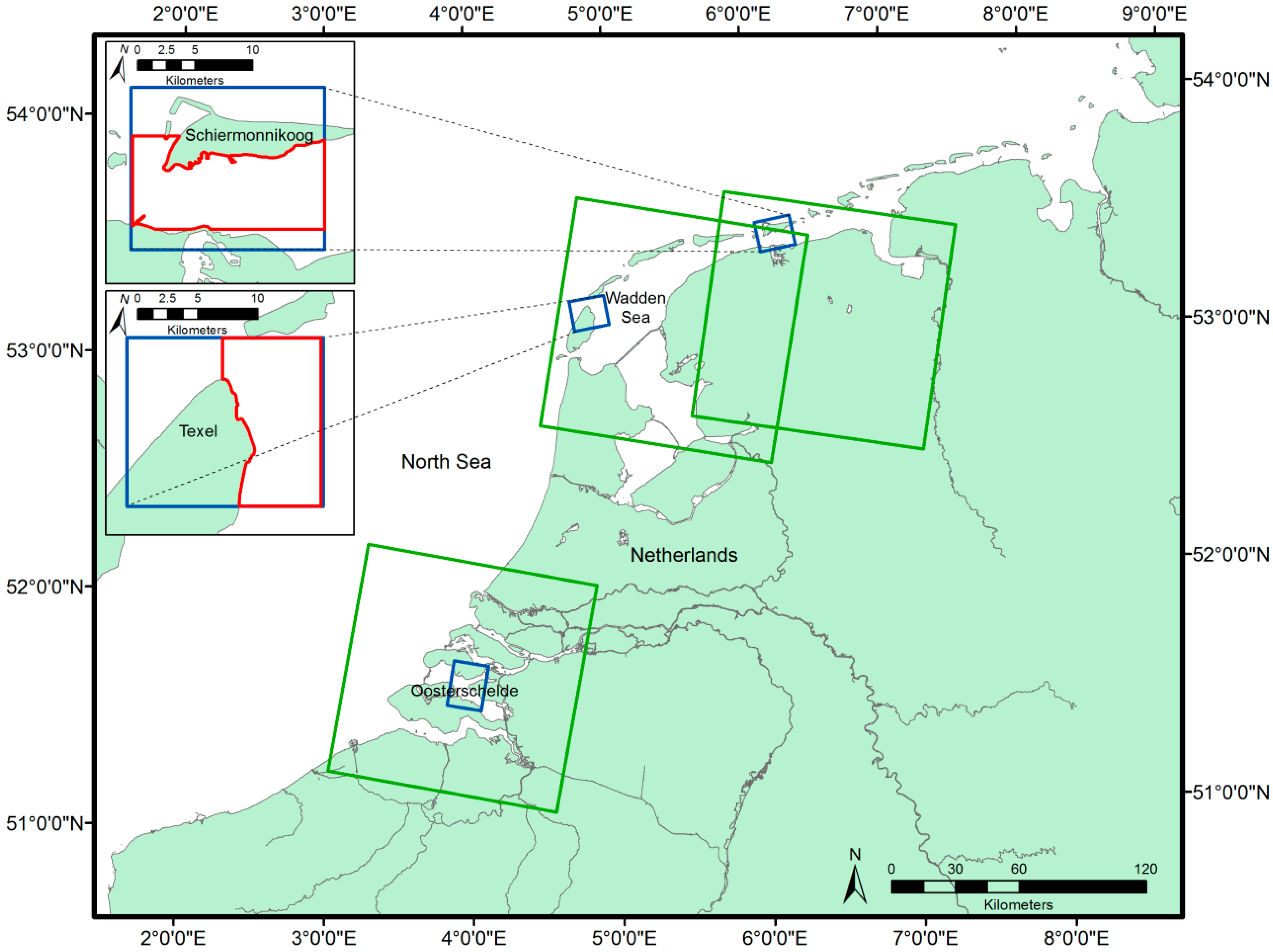
2.1. Study Areas

This study focused on two tidal systems in the Netherlands: the Wadden Sea and the Oosterschelde. The Wadden Sea is a mesotidal eutrophic marine system that is sheltered from the North Sea by a coastal barrier. The Wadden Sea was designated a UNESCO world natural heritage site in 2009 because of its dynamic intertidal zones, which are important foraging grounds for birds (111,882 ha of intertidal flats in the Dutch part [22]), and its diversity, which provides a suitable place for many organisms to reproduce and thrive [23,24]. However, in the last few decades, the Wadden Sea has been subjected to different forms of human-induced stress, which caused the disappearance of mussel beds in Dutch and German parts of the Wadden Sea in the 1980s [12,25]. After the collapse, the Dutch mussel fishery was restricted to subtidal beds in the western Wadden Sea, which resulted in recovery on the intertidal beds. Since then, mussel beds have recovered, but not to the extent reported in the 1970s [26]. In contrast to the mussel, the Pacific oyster is an invasive species in Dutch coastal waters that found its way from Zeeland to the Wadden Sea (Texel) for the first time in the late 1970s [8], but started increasing exponentially from the mid-1990s [27].

The Oosterschelde is a macrotidal system that is heavily influenced by human engineering; since 1986, a storm surge barrier has reduced the tidal prism in the system, resulting in a different hydrodynamic regime and changed sediment dynamics [28]. In 2001, 10,430 hectares of intertidal flat remained in the Oosterschelde estuary [29]. Mussels are cultivated in the Oosterschelde subtidally, but wild mussel beds have been virtually absent for decades. Pacific oysters were introduced in 1964 and have expanded rapidly since the 1970s, forming dense reefs in mainly the lower intertidal zone [8].

Two field sites were used within the Wadden Sea for this study, namely the mudflats east of the island of Texel and south of the island of Schiermonnikoog; one field site was used within the Oosterschelde (see Figure 1).

The flats consist of mostly sand and mud. Fragments of macroalgae can be present: their cover in the 107 sample plots of 1 m² used in this study was on average 7%. Areas with saltmarsh can also fringe some of the barrier islands and the mainland coast. Saltmarsh could potentially also be picked up with SAR satellites due to its complicated rough surfaces. However, we only focused on shellfish and did not include saltmarsh areas in this study, because saltmarsh has a more distinct optical signature, making it easier to classify using optical remote sensing.

2.2. SAR Imagery Acquisition and Preprocessing

Throughout 2012, three TerraSAR-X scenes were acquired through the German Aerospace Center (DLR), in strip map mode with a dual-polarization (VV and VH). In addition, three Radarsat-2 scenes were acquired (HH/HV) through the Dutch Satellietdataportaal (see Table 1). TerraSAR-X products were geocoded and ellipsoid corrected (GEC). Radiometric calibration of TerraSAR-X data was achieved by computing sigma nought ($\text{σ}°$) following product documentation [30]. Since the studied mudflats are more or less flat, we assumed a 0$°$ local incidence angle for all locations. Following radiometric calibration, images were filtered to reduce speckle using Lee’s refined adaptive local filter (7 × 7 moving window, with an edge threshold of 5000) [31], and pixel intensities were converted to decibels (dB).

Figure 1. Image acquisitions by Radarsat-2 (green) and by TerraSAR-X (blue) in the Netherlands. The red lines indicate the areas used to compare remotely-sensed and Trilateral Monitoring and Assessment Program (TMAP) shellfish maps.

Figure 1. Image acquisitions by Radarsat-2 (green) and by TerraSAR-X (blue) in the Netherlands. The red lines indicate the areas used to compare remotely-sensed and Trilateral Monitoring and Assessment Program (TMAP) shellfish maps.

Radarsat-2 products contained single look complex (SLC) data and were first multilooked 4 times in the azimuth direction. Radarsat-2 imagery was ellipsoid corrected, during which pixels were resampled using bilinear interpolation. The speckle filter used for Radarsat-2 imagery was similar to the one used for TerraSAR-X, and the same settings were used. Finally, pixel intensities were converted into decibels (dB). All SAR data processing was performed using the software package NEST 5.0.12. The average noise floor, noise equivalent sigma nought, was calculated for both image types, using the noise data provided with the satellite imagery.

Table 1. Specification of the different SAR scenes, the local prevailing conditions and matching field campaigns. The weather conditions were acquired from the Royal Netherlands Meteorological Institute (KNMI). Information on tidal conditions was provided by Rijkswaterstaat, the Dutch agency for water management. SLC is single look complex.

Ground Truth Date and Sample Size n	Satellite/Band	Image Date and Time	Image Type	Image Resolution (m)	Center (Lat/Lon, Degrees)	Incidence Angle (Degrees)	Polarization	Pass Direction	Water Height (m AOD *)	Tidal Stage	Wind Direction (Degrees)	Wind Speed (m/s)
Schiermonnikoog
24 August 2012 (n = 31) and 30 October 2012 (n = 26)	TSX/X	8 May 2012 17:18	Strip-map	3	53.46/6.20	39.75	VV/VH	Ascending	−0.41	outgoing	328	7.8
	RS2/C	23 May 2012 5:53	SLC	25	53.08/6.51	33.84	HH/HV	Descending	−1.34	low	56	6.8
Texel
18 September 2012 (n = 25) & 17 October 2012 (n = 15)	TSX/X	30 March 2012 17:27	Strip-map	3	53.08/4.87	42.71	VV/VH	Ascending	−0.68	outgoing	310	7.8
	RS2/C	27 July 2012 5:57	SLC	25	53.07/5.47	33.84	HH/HV	Descending	−0.69	outgoing	54	5.3
Galgenplaat
4 October 2012 (n = 10)	TSX/X	18 April 2012 6:00	Strip-map	3	51.59/3.98	38.79	VV/VH	Descending	−0.42	outgoing	166	7
	RS2/C	2 June 2012 6:01	SLC	25	51.62/3.95	33.86	HH/HV	Descending	−0.82	outgoing	57	3.6

* AOD is the Amsterdam Ordnance Datum.

Table 1. Specification of the different SAR scenes, the local prevailing conditions and matching field campaigns. The weather conditions were acquired from the Royal Netherlands Meteorological Institute (KNMI). Information on tidal conditions was provided by Rijkswaterstaat, the Dutch agency for water management. SLC is single look complex.

Ground Truth Date and Sample Size n	Satellite/Band	Image Date and Time	Image Type	Image Resolution (m)	Center (Lat/Lon, Degrees)	Incidence Angle (Degrees)	Polarization	Pass Direction	Water Height (m AOD *)	Tidal Stage	Wind Direction (Degrees)	Wind Speed (m/s)
Schiermonnikoog
24 August 2012 (n = 31) and 30 October 2012 (n = 26)	TSX/X	8 May 2012 17:18	Strip-map	3	53.46/6.20	39.75	VV/VH	Ascending	−0.41	outgoing	328	7.8
	RS2/C	23 May 2012 5:53	SLC	25	53.08/6.51	33.84	HH/HV	Descending	−1.34	low	56	6.8
Texel
18 September 2012 (n = 25) & 17 October 2012 (n = 15)	TSX/X	30 March 2012 17:27	Strip-map	3	53.08/4.87	42.71	VV/VH	Ascending	−0.68	outgoing	310	7.8
	RS2/C	27 July 2012 5:57	SLC	25	53.07/5.47	33.84	HH/HV	Descending	−0.69	outgoing	54	5.3
Galgenplaat
4 October 2012 (n = 10)	TSX/X	18 April 2012 6:00	Strip-map	3	51.59/3.98	38.79	VV/VH	Descending	−0.42	outgoing	166	7
	RS2/C	2 June 2012 6:01	SLC	25	51.62/3.95	33.86	HH/HV	Descending	−0.82	outgoing	57	3.6

* AOD is the Amsterdam Ordnance Datum.

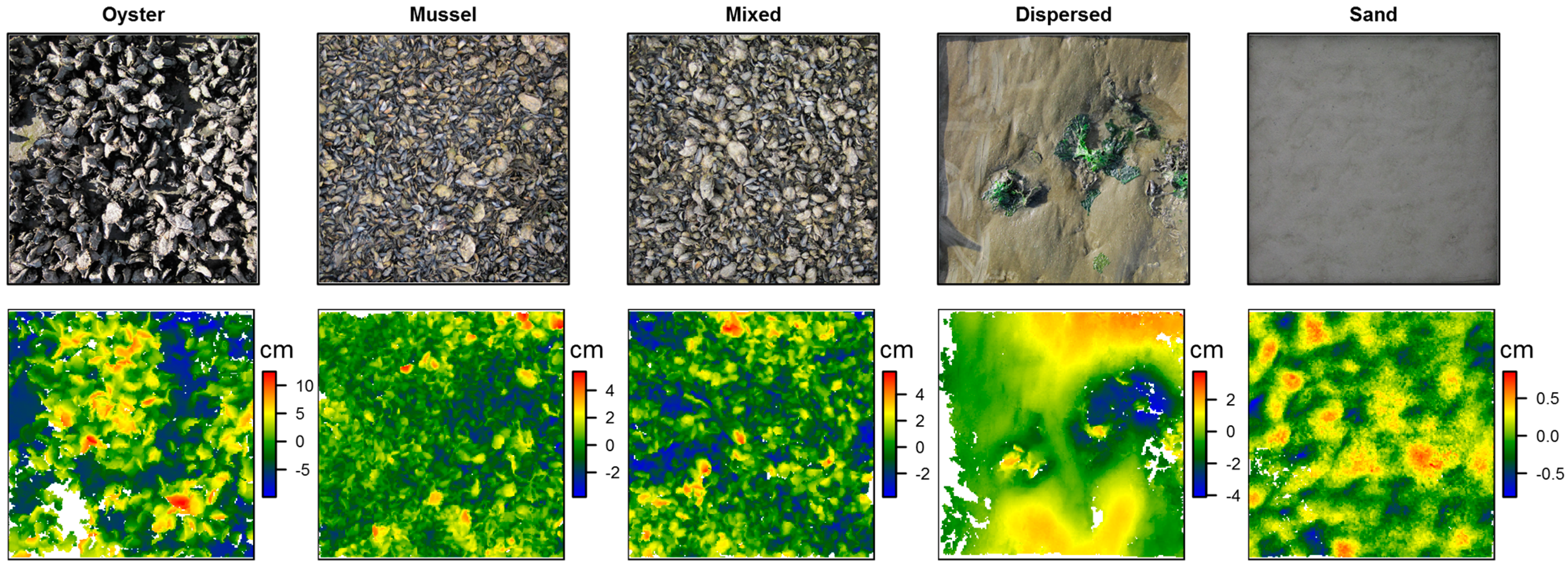
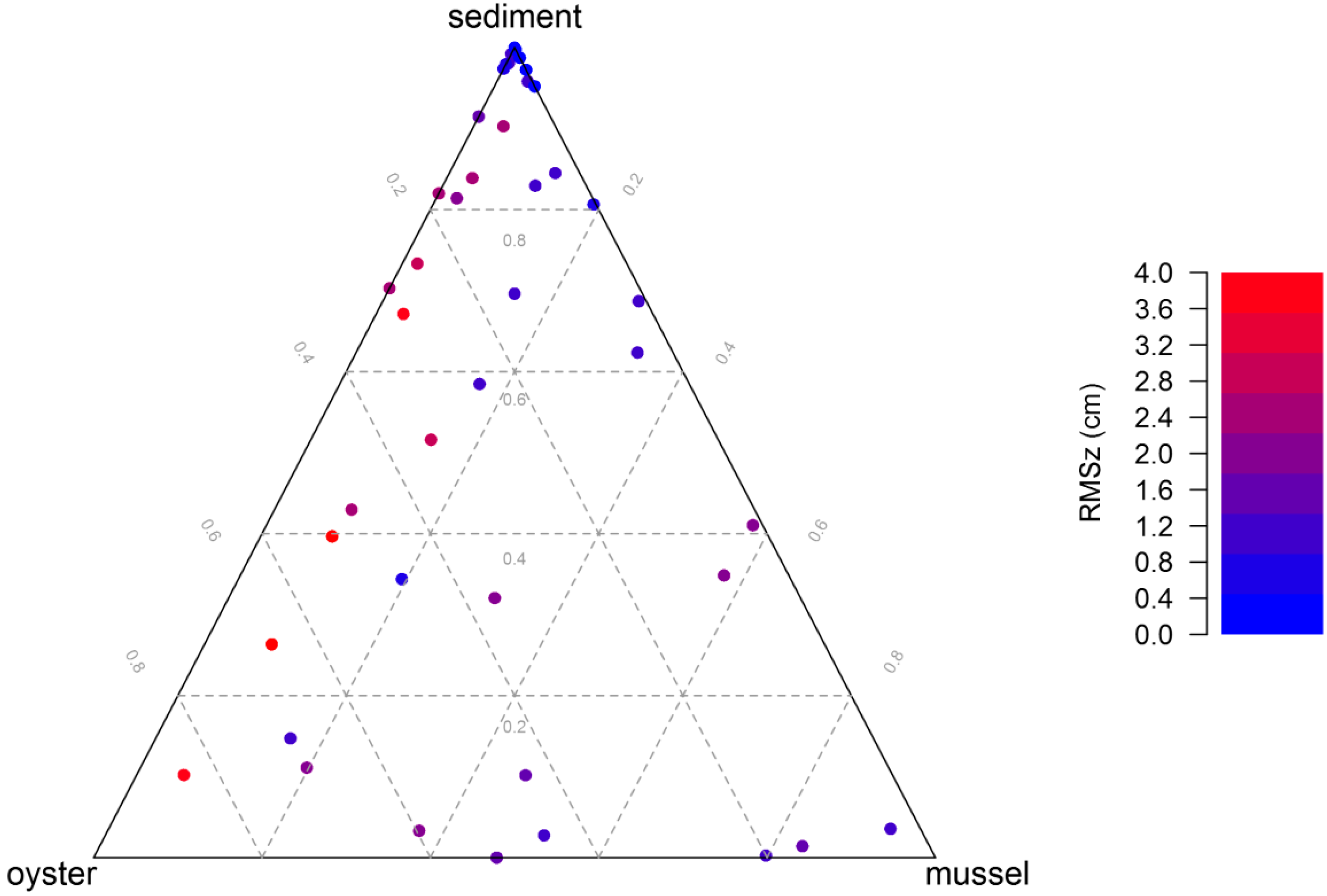
2.3. In Situ Surface Roughness Measurements

Each image was matched with the ground campaigns in that area (Table 1). Ground surveys did not coincide with satellite overpass, because sufficient light was required during the ground truth campaign, while satellite overpass occurs during either the beginning or the end of the day, and both field and image data had to be acquired when the tidal flat emerged. However, caution was taken that there were no severe weather conditions, like storms, in between. To determine the location of sample stations for ground-truthing over the full range of surface characteristics, iso cluster analysis was performed on TerraSAR-X imagery for both shellfish beds and bare mudflat surrounding the shellfish. To avoid sampling noise and to take into account positioning accuracies, the clusters were clumped and sieved in Erdas IMAGINE 2011 to retain clusters of at least 64 m². These zones were sampled using a random sample approach, in which the samples were at least 30 m apart, and the number of samples per zone was related to the total surface area of each zone. This resulted in a total of 107 samples (see Table 1 for the distribution of samples over the study areas).

The sample stations were located in the field using Garmin’s GPSmap 78 (average error in open sky conditions of 1.5 m; [32]). At each station, a 1-m² frame was used to mark the sampling surface, and a single photo was taken of the frame using either a Canon D10 or D20 camera. This photograph was subsequently used for cover analysis: first, the photo of the frame was transformed in ArcGIS 10.1, so that a 0.2 × 0.2 m grid could be projected on to it; then, different cover classes were derived and quantified from this grid as cover percentage, including sediment, oyster, mussel and total epibenthic shellfish cover.

Another 60 to 100 photographs per frame were taken using Canon 10D and 20D cameras at a height of about 50 to 60 cm, making sure that the entire frame was covered with abundant overlap between the pictures. With VisualSFM [33], these pictures were used to create a 3-dimensional representation of the frame and the surface by producing a set of data points with X, Y and Z coordinates: termed a point cloud. The point cloud was georeferenced using the corners of the frame as ground control points. A flat texture (carpet) was used to check the accuracy of the method; the planimetric and vertical root mean square error (RMSE) of this method were 0.931 cm and 0.240 cm, respectively. The vertical RMSE was largely due to a slight curvature in the measured plane, i.e., a difference with a second degree polynomial surface would result in a much lower vertical RMSE of 0.064 cm; thus, this method allows for a good comparison of roughness parameters between plots.

Commonly, in surface roughness measurements for SAR backscatter modelling, the root mean square height (RMSz) and correlation length (L) are derived to describe the vertical and horizontal component of surface roughness, respectively [34]. A mean plane was fitted to the height (Z) parameter of the point cloud and subtracted from the points. Using these detrended Z values, the root mean square height (RMSz) was calculated. To compute the correlation length, the point clouds were first rasterized to a 5 × 5 mm grid to calculate a 2-dimensional spatial autocorrelation function (ACF) [35], which, at location (x,y), is defined by:

$$\text{ACF}\left(\text{x},\text{y}\right)=\frac{{{\displaystyle \sum }}_{\text{i}=1}^{\text{N}-\text{x}}{{\displaystyle \sum }}_{\text{j}=1}^{\text{N}-\text{y}}\left({\text{h}}_{i,j}-\overline{{\text{h}}_{i,j}}\right)\times ({\text{h}}_{\text{i}+\text{x},\text{j}+\text{y}} - \overline{{\text{h}}_{\text{i},\text{j}}})}{{{\displaystyle \sum }}_{\text{i}=1}^{\text{N}-\text{x}}{{\displaystyle \sum }}_{\text{j}=1}^{\text{N}-\text{y}}{\left({\text{h}}_{i,j}-\overline{{\text{h}}_{i,j}}\right)}^2}$$

(1)

In which N is the number of cells in the grid in the X and Y direction (N = 200), h is the height grid, $\overline{\text{h}}$ is the height grid mean and ${\text{h}}_{\text{i}+\text{x},\text{j}+\text{y}}$ is the displaced grid at a lag location defined by X and Y. The 2D ACF grid was then transformed to a 1D ACF by calculating the mean (omnidirectional) autocorrelation over different lag distances with 1-mm increments. Horizontal surface roughness was expressed as the correlation length (L), which is the lag distance where the 1D ACF is 1/e [34]. Thus, values for RMSz and L were obtained for all 107 field plots. The omnidirectional measurement of surface roughness measurements was used, because most plots were isotropic. Anisotropy did occur in plots where shellfish beds are patchy in appearance, but these surfaces are expected to be isotropic at sensor resolution. This is because if a single patch does not fit in the 1-m² frame, it may still fit well in a sensor pixel. In these cases, an omnidirectional estimation of the roughness parameters is expected to give a more accurate representation of surface roughness at sensor resolution, compared to a directional estimation. In addition, the surface plot methods explained here typically contain many more measurements (in the order of millions), compared to the more traditional profile measurements, which increases the accuracy of roughness derivation further. For this study, a frame length of 1 m (with a maximum distance of $\sqrt{2}$ over which L is evaluated) was chosen to capture the roughness parameters. For longer lengths, height differences induced by mussel and oyster hummocks may affect the roughness parameters.

All spatial data were accumulated in a geographical information system (GIS). Statistical analyses described in the next paragraphs were performed using the statistical software package R [36], using a 0.05 significance level as a rejection criterion.

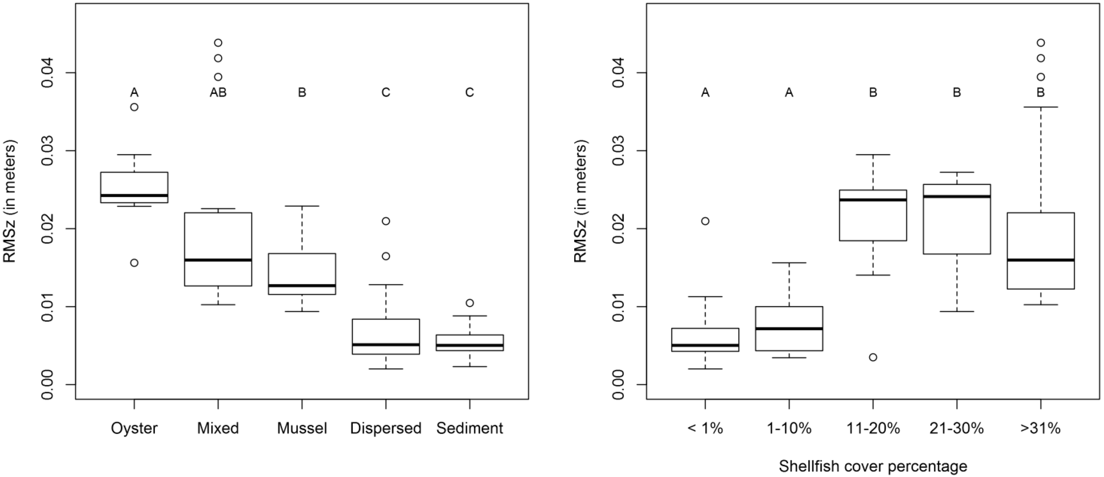
2.4. Effect of Shellfish Species and Cover on Surface Roughness and Backscatter

To test the effect of shellfish cover on surface roughness characteristics, the photos of the 1-m² frame were used to determine total shellfish cover (<1%, 1%–10%, 11%–20%, 21%–30%, >30%). In addition, five substrate types were distinguished based on Troost et al. [37], namely sediment (no shellfish present), dispersed shellfish (less than 5% cover by both mussels and oysters), mussel (less than 5% surface covered by oysters and more than 5% by mussels), mixed (both shellfish cover more than 5%) and oyster (less than 5% surface covered by mussels and more than 5% by oysters) (see Figure 2). After classification, 10 samples were classified as oyster, 15 as mixed, 8 as mussel, 41 as dispersed shellfish and 33 as sediment. Analysis of variance in combination with the Tukey HSD post hoc tests were used to test if differences in total shellfish cover and differences in substrate type had a significant impact on surface roughness in terms of RMSz and L and whether they had an effect on radar backscatter.

2.5. Shellfish Backscatter Modelling and Mapping

To explore the backscatter signal in response to roughness elements in the tidal flat and to investigate the potential for surface characteristic retrieval from backscatter, we investigated the response and validity of three backscatter models over the roughness range that we observed in this study. The first two models are theoretical (the integral equation model) and semi-empirical (Oh’s model), and aim to predict backscatter based on surface characteristics and sensor settings. The third model is empirical (based on logistic regression) and can only be used for mapping shellfish beds.

Figure 2. The top row shows examples of photos of the different substrate classes studied in the 1-m² plots. The bottom row shows corresponding examples of the measured height after rasterization of the point clouds at a resolution of 5 mm.

Figure 2. The top row shows examples of photos of the different substrate classes studied in the 1-m² plots. The bottom row shows corresponding examples of the measured height after rasterization of the point clouds at a resolution of 5 mm.

The integral equation model, or IEM [18], is commonly used to predict backscatter from surface parameters in intertidal environments (root mean square height, correlation length and dielectric constant) and SAR configuration (polarization of microwave signal, wavelength and angle of incidence) [14,38,39,40]. In this study, we used an extended version of the IEM that takes into account the phase effect in Green’s function; as a result, this version provides much more accuracy in bistatic scattering and also includes multiple scattering [41]; an elaborate description of the model can be found in Fung and Chen [42]. For this study, we used a spectrum with an exponential autocorrelation function. High moisture contents are typical for shellfish habitats due to the high amounts of silt in the sediment. We used a large number of samples (n = 175) of the upper 3 cm of the surface from a field campaign in the Wadden Sea in 2013 to determine that the average volumetric moisture content of the sediment during low tide is 0.45 (±0.09) cm³/cm³. Assuming this average value and taking into account the grain-size distribution of the sediment, a dielectric constant of ε = 29.31 + 12.72i and 35.67 + 9.55i was calculated for the X-band and C-band, respectively, following Hallikainen et al. [43]. The validity range of the IEM is given by RMSz/L < 0.4 and k × RMSz < 3, where k is the wavenumber (2 × π/λ). Using the IEM, we simulated radar backscatter over a range of RMSz and L found in the field campaign for co- and cross-polarized channels in X- and C-band.

Since the validity range of the IEM is easily exceeded (i.e., k × RMSz > 3, which translates to a threshold of RMSz of 1.5 cm for X-band and 2.65 cm for C-band), we also used Oh’s semi-empirical model described in [44]. This semi-empirical model was fit using data from bare surfaces and was tested to be valid up to 6.98 [44] for k × RMSz (which translates to a threshold RMSz of 3.5 cm for the X-band and a threshold RMSz of 6.23 cm for the C-band) over incidence angles between 10° and 70°. Using this model, backscatter can be expressed as a function of RMSz, volumetric moisture content, incidence angle, wavelength and polarization. Since the simulations consequently overestimated radar backscatter based on the volumetric moisture content of 0.45, the model was also fit using nonlinear least squares based on the Gauss–Newton algorithm to determine the best fit volumetric moisture content. Based on this approach the estimated moisture contents were 0.04 and 0.13 cm³/cm³ for X-band VV and VH, respectively, and 0.06 and 0.15 cm³/cm³ for C-band HH and HV, respectively. This model was used to predict backscatter over the range of RMSz that was found in this study for co- and cross-polarized channels in the X- and C-band.

For mapping purposes of intertidal shellfish beds, it may be sufficient to discriminate between shellfish and bare sediment patches. We used a logistic model to build three classifiers for both TerraSAR-X and Radarsat-2 for co- and cross-polarized channels separately. To distinguish between sediment, sediment with dispersed shellfish (where total shellfish cover <5%, n = 70), and shellfish (where total shellfish cover > 5%, n = 37) classes, a multivariate logistic regression was used for a dual-polarized classification. An additional classifier based on the two single-channel thresholds was also investigated, because this will likely be less sensitive to rough rippled sediments, which were rare in the training data. The level of 5% shellfish was chosen in line with the protocol described in the TMAP procedure. The univariate logistic function $P(\text{x})$ can be written as:

$$P(x)= \frac{1}{1+ e^{-({\text{β}}_0+{\text{β}}_{1}x)}}$$

(2)

This equation was used to determine at which backscatter value a pixel would have equal probabilities (i.e., P = 0.5) to be classified as shellfish or sediment in a single channel. The threshold value can be calculated using:

$$x\left(P=0.5\right)= \frac{-{\text{β}}_0}{{\text{β}}_1}$$

(3)

In the dual polarized classification, we expanded the logistic function to incorporate both channels. In this case, the threshold value in the cross-polarized channel can be found for any given backscatter value in the co-polarized channel using:

$${{\text{σ}}^{°}}_{crosspol}= \frac{-({\text{β}}_0+{\text{β}}_2{{\text{σ}}^{°}}_{copol} )}{{\text{β}}_1}$$

(4)

Pixels were classified as shellfish when the threshold values were surpassed. Contingency tables were calculated to assess the performance of the three classifiers using different accuracy metrics [45], which include Kappa, sensitivity, specificity, precision and accuracy.

2.6. Comparing Shellfish Maps from SAR with Traditional Field Surveys

To determine how well the classification compares to traditional field surveys, we compared the results of the classification of Radarsat-2 and TerraSAR-X data with an extensive ground survey based on the TMAP protocol performed in 2012 in which oyster and mussel beds were mapped in the Wadden Sea [46]. The 2012 TMAP monitoring results in a polygon feature layer covering the area under investigation in this project. The polygons were converted to raster data matching the spatial resolution of the SAR data, so that contingency tables could be computed. In case both sediment and shellfish were present in a cell, the majority rule was used to assign the raster value. An area of interest was defined in such a way that it excluded land (and salt-marshes), yet it still occupied large parts of the Wadden Sea to the east of Texel and south of Schiermonnikoog (see Figure 1). From these areas, contingency tables were calculated, which were subsequently used to derive the same classification scores as described for the classifier to see how well the remotely-sensed data match with the ground survey data. Classification scores of how the SAR classification compares with the field survey campaigns were calculated separately for the eastern and western Wadden Sea, because these areas might be quite different when it comes to sediment texture and the prevalence and patchiness of shellfish beds.

3. Results and Discussion

3.1. Effect of Shellfish Species and Cover on Surface Roughness

The analysis of variance on substrate types showed that there was a significant effect of substrate class on RMSz (F_{4, 102} = 45.07, p < 0.001) (left graph in Figure 3). The Tukey HSD post hoc test showed that dispersed shellfish and sediment plots have lower RMSz than the shellfish-dominated plots and that oyster plots have higher RMSz than mussel plots (left graph in Figure 3). The ANOVA also reveals a significant effect of shellfish density on RMSz (F_{4, 102} = 30.74, p < 0.001); the right graph in Figure 3 shows that high total shellfish cover (density) is generally associated with high RMSz values and low cover with low RMSz values, with a rather abrupt switch at lower shellfish covers. Results of the Tukey HSD post hoc test confirm that the lower shellfish cover classes (<1% and 1%–10%) had a significantly different RMSz than the higher cover classes (10%–20%, 20%–30%, >30%) (right graph in Figure 3). Figure 4 shows that surface roughness is mainly driven by oysters if they are present; however, the presence of mussels can actually decrease surface roughness, as these bivalves fill cracks and crevices efficiently.

Figure 3. (Left) RMSz for oyster, mixed, mussel, dispersed and sediment plots (shellfish classes significantly different from dispersed and sediment at p < 0.05); (Right) RMSz as a function of shellfish cover: RMSz in cover classes < 1% and 1%–10% significantly differed from that in classes 11%–20%, 21%–30% and >21% (p < 0.05). Letters indicate homogeneous groups based on the Tukey HSD test. In the boxplots, the rectangles of the boxes show the interquartile range, the bold bar the median and the whiskers the minimum and maximum values (without outliers).

Figure 3. (Left) RMSz for oyster, mixed, mussel, dispersed and sediment plots (shellfish classes significantly different from dispersed and sediment at p < 0.05); (Right) RMSz as a function of shellfish cover: RMSz in cover classes < 1% and 1%–10% significantly differed from that in classes 11%–20%, 21%–30% and >21% (p < 0.05). Letters indicate homogeneous groups based on the Tukey HSD test. In the boxplots, the rectangles of the boxes show the interquartile range, the bold bar the median and the whiskers the minimum and maximum values (without outliers).

Neither substrate type (F_{4, 102} = 1.63, p = 0.172) nor shellfish cover (F_{4, 102} = 1.804, p = 0.134) have a significant effect on correlation length. It is widely recognized that L is not scale invariant, and therefore, the values obtained are dependent on profile length and plot size [47,48,49]. Zribi and Dechambre [50] stated that neglecting L will result in large errors in estimating radar backscatter, and therefore, they proposed a new measure, called Zs, which incorporates a slope effect. Bretar et al. [49] showed that Zs behaved more or less scale invariant. Furthermore, tortuosity and fractal dimension also appeared to be scale-invariant descriptors of surface roughness [49]. These measures were not used in this study, because it is unclear how they can be incorporated in the backscatter models used here.

Figure 4. Ternary plot of RMSz between pure oyster, mussel and sediment cover fractions. RMSz values depend largely on the presence of oysters in the plot.

Figure 4. Ternary plot of RMSz between pure oyster, mussel and sediment cover fractions. RMSz values depend largely on the presence of oysters in the plot.

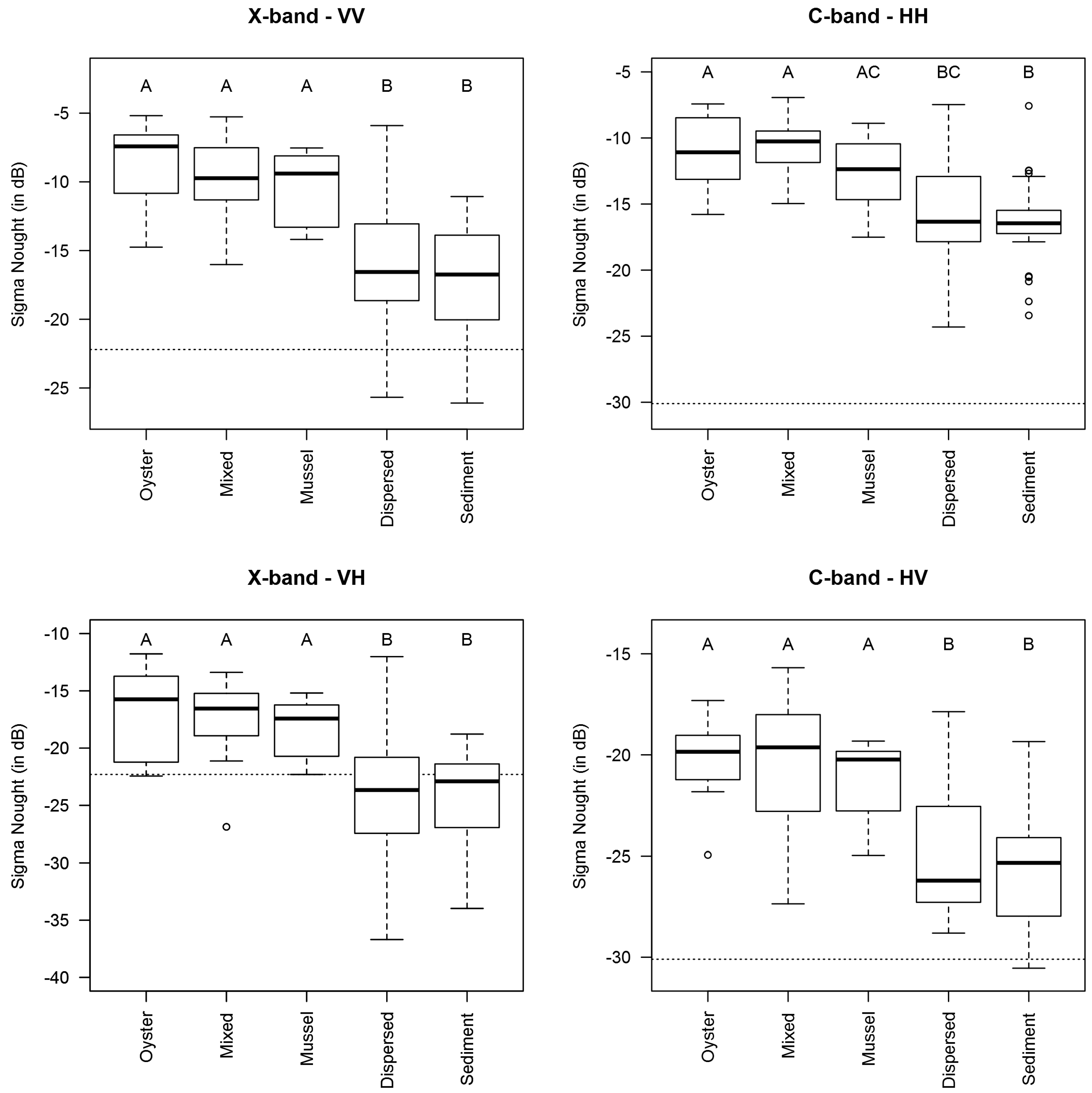
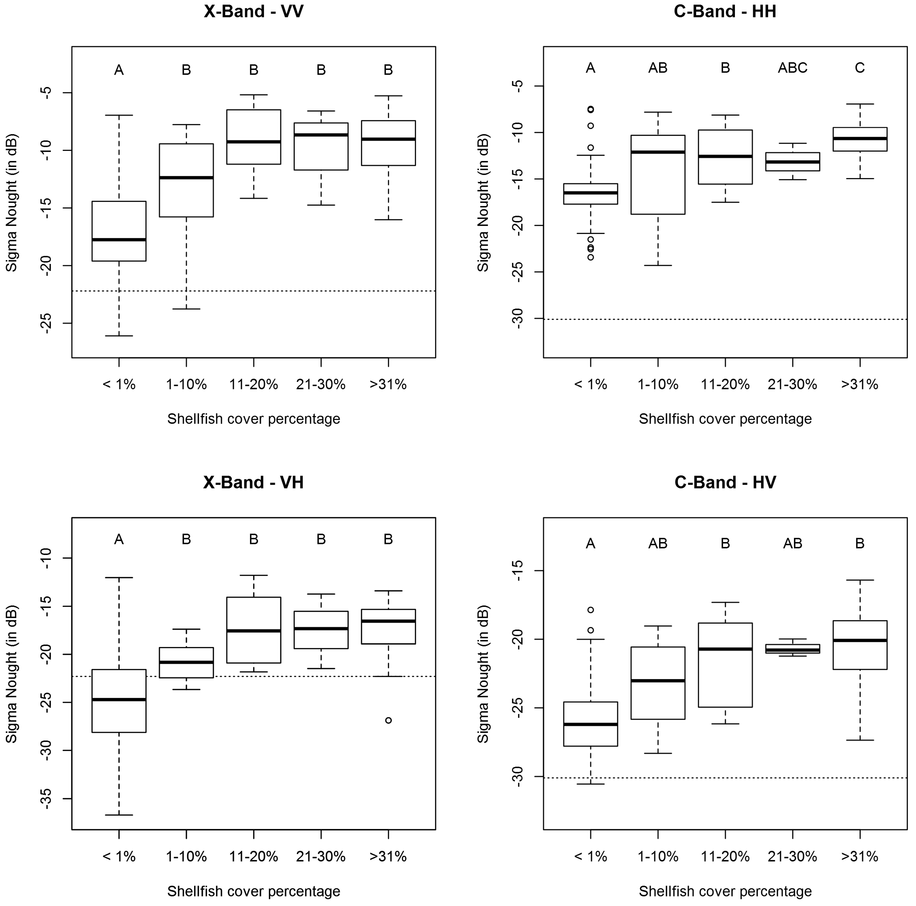
3.2. Effect of Surface Roughness and Shellfish Species and Cover on Radar Backscatter

In most backscatter channels, the shellfish substrates could clearly be distinguished from sediment and dispersed shellfish, but within shellfish beds, it was not possible to distinguish backscatter in mussel-dominated and oyster-dominated plots (Figure 5, Table 2). Backscatter saturates too quickly to distinguish species in radar imagery regardless of which wavelength was used. There was a clear trend for all backscatter channels that radar backscatter increases with increasing shellfish cover. However, due to the overlap of the different classes, as indicated by the Tukey HSD post hoc test, derivation of shellfish densities from radar backscatter is hard (Figure 6).

Both the X- and C-band SAR backscatter saturate at shellfish cover levels as low as 10%, corresponding to RMSz values as high as 1.5 cm. For future investigations, it is worth looking into data with lower incidence angles. This should decrease the strong effect of RMSz on backscatter slightly, although Choe et al. [15] found that it could result in less contrast between bare sediment and shellfish. Alternatively, longer SAR wavelengths may also improve backscatter resolution within the RMSz range typically found in the shellfish class.

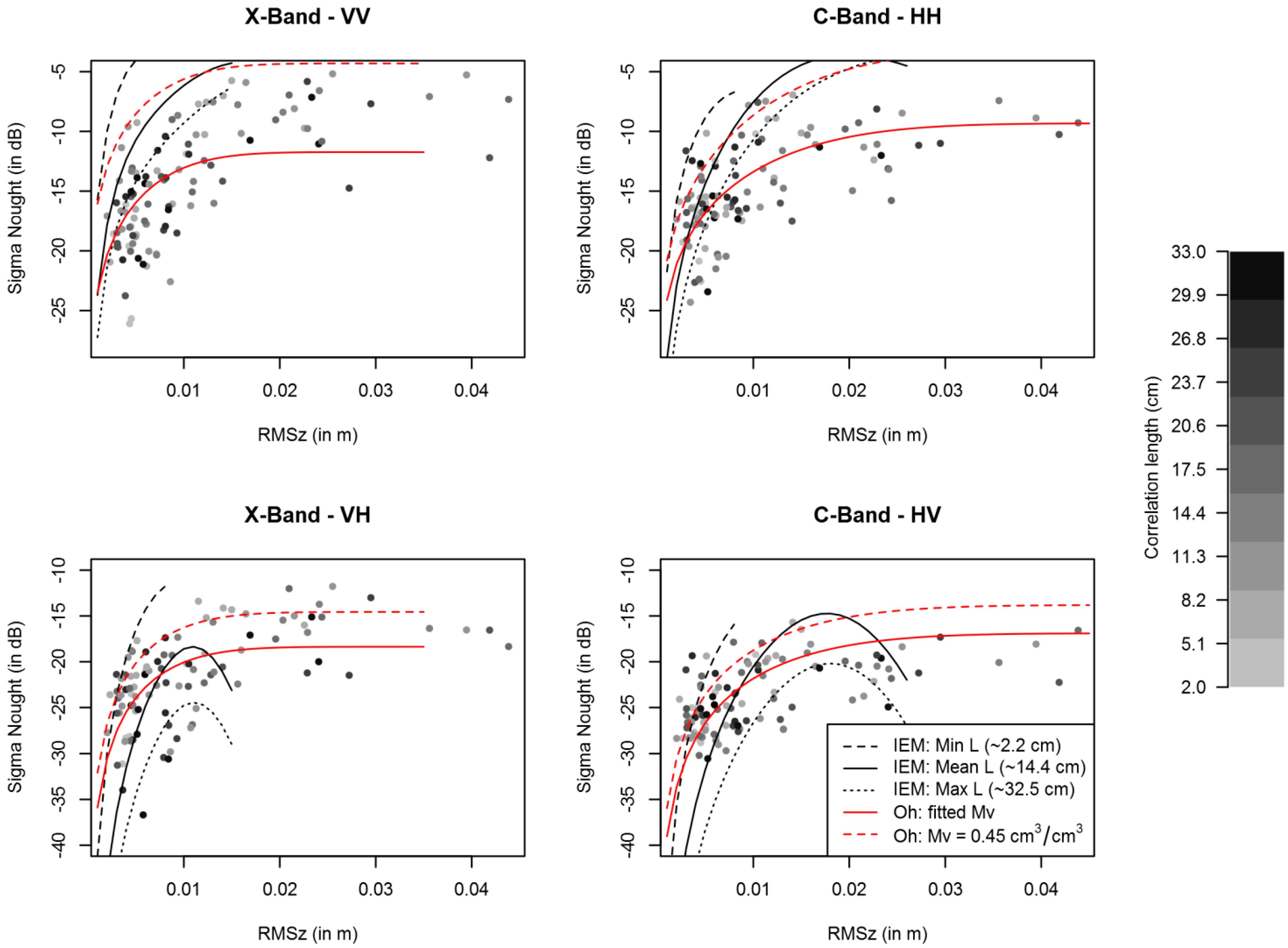
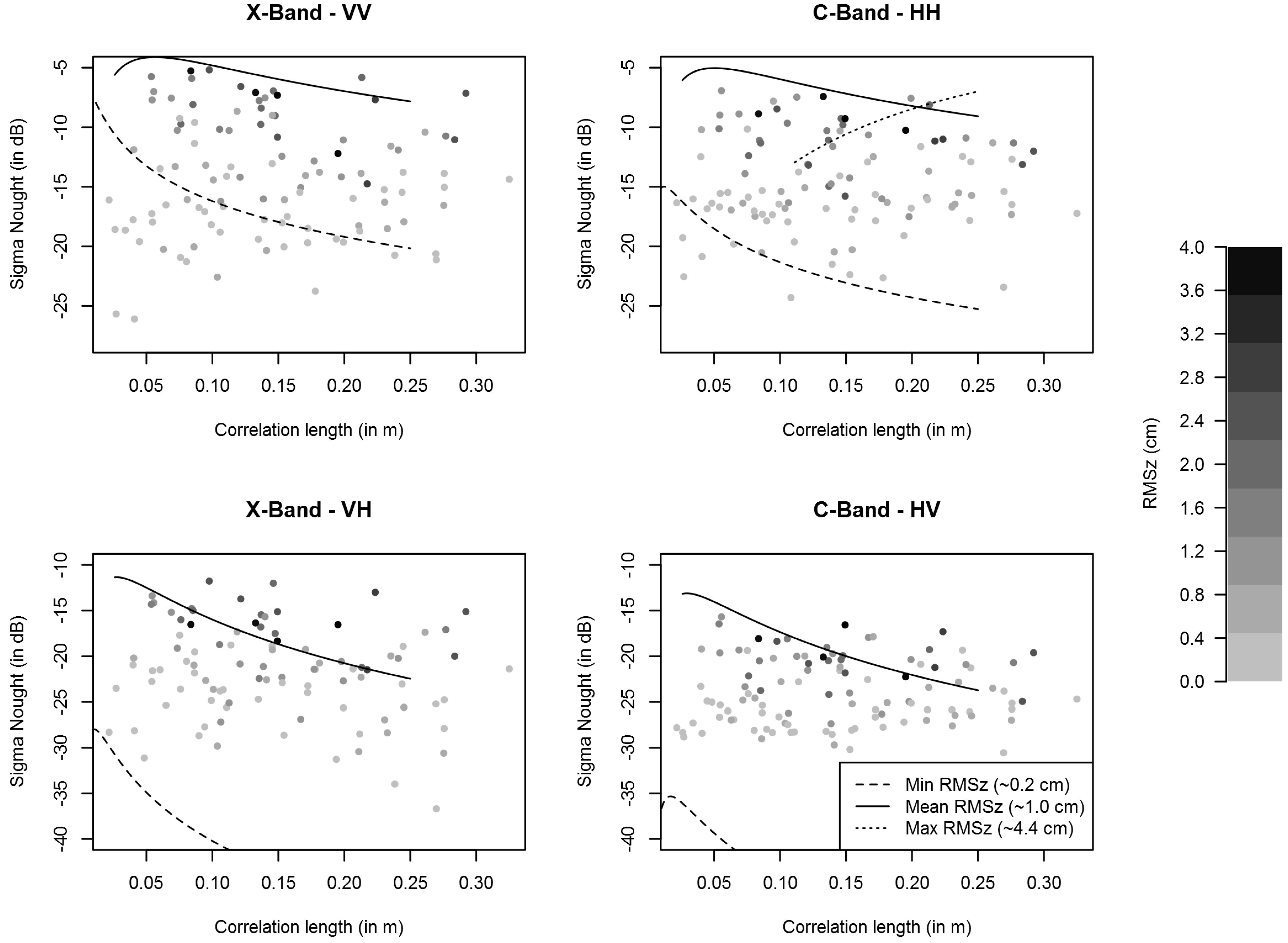
3.3. Theoretical and Semi-Empirical Simulation of Shellfish-Induced Backscatter

IEM predictions of the backscatter as a function of surface roughness RMSz and correlation length L were compared to observations at the 107 plots. First, the simulations were performed for RMSz, where we assumed correlation lengths L of 2.2, 14.4 and 32.5 cm for the IEM, which is respectively the minimum, mean and maximum L observed in this study. Our data range observed for RMSz exceeds the validity of the IEM in both the C- and X-band. We found that the IEM was rather accurate in predicting radar backscatter as a function of RMSz, especially in cross-polarized settings, given that L is assumed to be constant and provided that the model is only used within the validity range (Figure 7).

Figure 5. Plots with epibenthic shellfish significantly differed in backscatter from sediment and dispersed plots, but mussels, mixed and oysters do not differ significantly in backscatter. Letters indicate similar plots based on the Tukey HSD test. The dashed line indicates the average noise floor (noise equivalent sigma nought).

Figure 5. Plots with epibenthic shellfish significantly differed in backscatter from sediment and dispersed plots, but mussels, mixed and oysters do not differ significantly in backscatter. Letters indicate similar plots based on the Tukey HSD test. The dashed line indicates the average noise floor (noise equivalent sigma nought).

Table 2. ANOVA statistics of backscatter between different types of substrates (i.e., sediment, mussels and oysters) and ANOVA statistics of backscatter between different cover classes (densities) of shellfish.

Satellite	Channel	Substrate Type			Shellfish Cover
		D.f., N	F Statistic	Probability	D.f., N	F Statistic	Probability
TerraSAR-X	VV	4, 102	14.32	<0.001	4, 102	17.82	<0.001
TerraSAR-X	VH	4, 92	11.46	<0.001	4, 92	16.63	<0.001
Radarsat-2	HH	4, 102	11.95	<0.001	4, 102	12.56	<0.001
Radarsat-2	HV	4, 102	15.92	<0.001	4, 102	16.34	<0.001

Table 2. ANOVA statistics of backscatter between different types of substrates (i.e., sediment, mussels and oysters) and ANOVA statistics of backscatter between different cover classes (densities) of shellfish.

Satellite	Channel	Substrate Type			Shellfish Cover
		D.f., N	F Statistic	Probability	D.f., N	F Statistic	Probability
TerraSAR-X	VV	4, 102	14.32	<0.001	4, 102	17.82	<0.001
TerraSAR-X	VH	4, 92	11.46	<0.001	4, 92	16.63	<0.001
Radarsat-2	HH	4, 102	11.95	<0.001	4, 102	12.56	<0.001
Radarsat-2	HV	4, 102	15.92	<0.001	4, 102	16.34	<0.001

Figure 6. Boxplots showing the relationship between radar backscatter and shellfish cover. Letter codes indicate similarity based on the Tukey HSD test. The dashed line indicates the average noise floor (noise equivalent sigma nought).

Figure 6. Boxplots showing the relationship between radar backscatter and shellfish cover. Letter codes indicate similarity based on the Tukey HSD test. The dashed line indicates the average noise floor (noise equivalent sigma nought).

In the co-polarized channel, backscatter is overestimated. The difference observed between model predictions and in situ roughness observations could be due to the relatively small plot size used in the ground truth campaign. This probably overestimates RMSz in relation to surface roughness estimated by the SAR sensors, which evaluate surface roughness at a much larger spatial extent dependent on sensor resolution. Shellfish beds are often patchy in nature (see, for instance, [51]), which means that at larger spatial scales, which are used by the satellites, there is more chance of including flat mud and water in between the shellfish [52].

For all wavelengths and polarizations, and for all parameterizations of L, small variations in RMSz have large effects on the backscatter signal for relatively low values of RMSz, which is both predicted by the IEM model and observed. At higher RMSz levels, the IEM predicts a decreasing trend in radar backscatter. This effect is attributed to the fact that the angular curve becomes more isotropic at larger values of RMSz at these values of incidence angles [42]. Our data, however, show a saturating response at high RMSz values; we did not observe a decrease of backscatter, but a consistent high level associated with high RMSz (up to 4 cm), even outside of the validity range. Simulations of L using the IEM were calculated at minimum, mean and maximum values for RMSz (see Figure 8) and show that the observed values are within the range predicted by IEM. It also shows that there is hardly any variation in L with increasing backscatter, while it is clear that high backscatter values are associated with high RMSz values. Thus, the effect of L, as measured in the field, appears subordinate to the effect of RMSz.

Figure 7. Model simulations of backscatter (sigma nought) in the X-band (VV and VH polarizations) and C-band (HH and HV polarizations) show the effect of RMSz. For the integral equation model (IEM) simulations, minimum, mean and maximum correlation lengths were used. An incidence angle of 40° and 34° was assumed for TerraSAR-X and Radarsat-2 respectively. The dots in the graphs are actual observations of surface roughness in the field and their backscatter observed in radar imagery. The grey scale in the images gives an impression of the correlation length at the measured sample points. The red lines are simulations based on Oh’s model for varying moisture contents (solid red lines; see the text) and moisture content of 0.45 (dashed red lines). Lines are shown for the validity domain of the models.

Figure 7. Model simulations of backscatter (sigma nought) in the X-band (VV and VH polarizations) and C-band (HH and HV polarizations) show the effect of RMSz. For the integral equation model (IEM) simulations, minimum, mean and maximum correlation lengths were used. An incidence angle of 40° and 34° was assumed for TerraSAR-X and Radarsat-2 respectively. The dots in the graphs are actual observations of surface roughness in the field and their backscatter observed in radar imagery. The grey scale in the images gives an impression of the correlation length at the measured sample points. The red lines are simulations based on Oh’s model for varying moisture contents (solid red lines; see the text) and moisture content of 0.45 (dashed red lines). Lines are shown for the validity domain of the models.

Figure 8. IEM simulations of backscatter (sigma nought) in the X-band (VV and VH polarizations) and C-band (HH and HV polarizations) show the effect of L. For the IEM simulations, minimum, mean and maximum RMSz values were used. An incidence angle of 40° and 34° was assumed for TerraSAR-X and Radarsat-2, respectively. The dots in the graphs are actual observations of surface roughness in the field and their backscatter observed in radar imagery. The grey scale in the images gives an impression of RMSz at the measured sample points. Lines are shown for the validity domain of the models.

Figure 8. IEM simulations of backscatter (sigma nought) in the X-band (VV and VH polarizations) and C-band (HH and HV polarizations) show the effect of L. For the IEM simulations, minimum, mean and maximum RMSz values were used. An incidence angle of 40° and 34° was assumed for TerraSAR-X and Radarsat-2, respectively. The dots in the graphs are actual observations of surface roughness in the field and their backscatter observed in radar imagery. The grey scale in the images gives an impression of RMSz at the measured sample points. Lines are shown for the validity domain of the models.

The Oh [44] semi-empirical model does not include L, both because the cross-polarized ratio is relatively insensitive to changes in L and because of the problems of estimating L properly in the field [44]. Oh’s model did not predict a decrease in backscatter for higher RMSz values and performed well across the entire range of RMSz associated with both bare sediments and shellfish beds. The shape of the model matches quite well with the observations (Figure 7); however, model parameterization with observed moisture content largely overestimates the observed backscatter, whereas the best fit uses extremely low values for moisture content. It is therefore worth investigating the dielectric properties of the substrate in intertidal environments, including its constituents saline water and shells (calcium carbonate material). In addition, other factors, such as the fraction of surface water influencing roughness and the spatial extent of the roughness measurements in relation to that detected by the sensor, could have played a role.

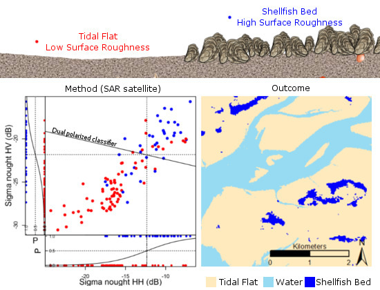
3.4. Shellfish Mapping Using SAR

Shellfish presence in major Dutch intertidal regions was mapped using an empirical classification approach. The classification revealed that a threshold on dual-polarized data calculated by class separation using logistic regression is a good method to map shellfish presence (Figure 9).

Figure 9. Plot showing the classification method based on the training set. (a) TerraSAR-X data and (b) Radarsat-2 data. The red points represent the class with <5% shellfish and the blue points the class with >5% shellfish. The marginal plots show the logistic regression that was used to find the threshold values (dotted lines) at the intersection, where the probability is 50% for single-polarized classifications. The solid line is the threshold value for the multivariate logistic regression for dual-polarized data. See Table 3 for the statistics.

Figure 9. Plot showing the classification method based on the training set. (a) TerraSAR-X data and (b) Radarsat-2 data. The red points represent the class with <5% shellfish and the blue points the class with >5% shellfish. The marginal plots show the logistic regression that was used to find the threshold values (dotted lines) at the intersection, where the probability is 50% for single-polarized classifications. The solid line is the threshold value for the multivariate logistic regression for dual-polarized data. See Table 3 for the statistics.

Table 3. Training statistics for the shellfish classifiers used. Thresholds (in dB) and statistics were calculated using logistic regression for co-polarized data (VV or HH), cross-polarized data (VH or HV), dual-polarized (DUAL) data and a combination of both single-band thresholds (VV + VH or HH + HV).

	TerraSAR-X				Radarsat-2
	VV	VH	DUAL	VV + VH	HH	HV	DUAL	HH + HV
Missing values	0	10	10	10	0	0	0	0
True Positives	29	26	31	25	24	25	26	22
True Negatives	64	53	54	57	62	59	60	63
False Positives	6	7	6	3	8	11	10	7
False Negatives	8	11	6	12	13	12	11	15
Sensitivity	0.78	0.70	0.84	0.68	0.65	0.68	0.70	0.59
Specificity	0.91	0.88	0.90	0.95	0.89	0.84	0.86	0.9
Precision	0.83	0.79	0.84	0.89	0.75	0.69	0.72	0.76
Accuracy	0.87	0.81	0.88	0.85	0.80	0.79	0.80	0.79
Kappa	0.71	0.60	0.74	0.66	0.55	0.52	0.56	0.52

Table 3. Training statistics for the shellfish classifiers used. Thresholds (in dB) and statistics were calculated using logistic regression for co-polarized data (VV or HH), cross-polarized data (VH or HV), dual-polarized (DUAL) data and a combination of both single-band thresholds (VV + VH or HH + HV).

	TerraSAR-X				Radarsat-2
	VV	VH	DUAL	VV + VH	HH	HV	DUAL	HH + HV
Missing values	0	10	10	10	0	0	0	0
True Positives	29	26	31	25	24	25	26	22
True Negatives	64	53	54	57	62	59	60	63
False Positives	6	7	6	3	8	11	10	7
False Negatives	8	11	6	12	13	12	11	15
Sensitivity	0.78	0.70	0.84	0.68	0.65	0.68	0.70	0.59
Specificity	0.91	0.88	0.90	0.95	0.89	0.84	0.86	0.9
Precision	0.83	0.79	0.84	0.89	0.75	0.69	0.72	0.76
Accuracy	0.87	0.81	0.88	0.85	0.80	0.79	0.80	0.79
Kappa	0.71	0.60	0.74	0.66	0.55	0.52	0.56	0.52

The performance of the classification training is given in Table 3. Generally, the specificity of SAR classification is slightly higher than the sensitivity, meaning that it is easier to classify bare sediments correctly, but this effect is affected by the overrepresentation of bare sediment. Kappa values, which take into account the probability of representation of bare sediment and shellfish pixels, show that all classifiers separate data with moderate to substantial performance according to Landis and Koch [53]. In general, the maps based on the dual-polarized multivariate classification, as well as the classifier that uses both single-band thresholds, perform better than single-band classifiers. TerraSAR-X performs better than Radarsat-2, e.g., Kappa = 0.74 for TerraSAR-X and Kappa = 0.56 for Radarsat-2, using the dual-polarized multivariate classification. For an overview of the threshold parameters, please refer to Table 4.

Table 4. Pixel thresholds to qualify as shellfish for the different classifiers for TerraSAR-X and Radarsat-2.

	Classifier	Thresholds (in dB)
TerraSAR-X	VV	${{\text{σ}}^{°}}_{\text{VV}}> -11.85$
	VH	${{\text{σ}}^{°}}_{\text{VH}}> -19.75$
	DUAL	${{\text{σ}}^{°}}_{\text{VH}}> \frac{-(8.42+0.44{{\text{σ}}^{°}}_{\text{VV}})}{0.16}$
	VV + VH	$({{\text{σ}}^{°}}_{\text{VV}}> -11.85) \& ({{\text{σ}}^{°}}_{\text{VH}} > -19.75)$
Radarsat-2	HH	${{\text{σ}}^{°}}_{\text{HH}}> -12.34$
	HV	${{\text{σ}}^{°}}_{\text{HV}}> -21.82$
	DUAL	${{\text{σ}}^{°}}_{\text{HV}}> \frac{-(9.94+0.09{{\text{σ}}^{°}}_{\text{HH}})}{0.41}$
	HH + HV	$({{\text{σ}}^{°}}_{\text{HH}}> -12.34) \& ({{\text{σ}}^{°}}_{\text{HV}} > -21.82)$

Table 4. Pixel thresholds to qualify as shellfish for the different classifiers for TerraSAR-X and Radarsat-2.

	Classifier	Thresholds (in dB)
TerraSAR-X	VV	${{\text{σ}}^{°}}_{\text{VV}}> -11.85$
	VH	${{\text{σ}}^{°}}_{\text{VH}}> -19.75$
	DUAL	${{\text{σ}}^{°}}_{\text{VH}}> \frac{-(8.42+0.44{{\text{σ}}^{°}}_{\text{VV}})}{0.16}$
	VV + VH	$({{\text{σ}}^{°}}_{\text{VV}}> -11.85) \& ({{\text{σ}}^{°}}_{\text{VH}} > -19.75)$
Radarsat-2	HH	${{\text{σ}}^{°}}_{\text{HH}}> -12.34$
	HV	${{\text{σ}}^{°}}_{\text{HV}}> -21.82$
	DUAL	${{\text{σ}}^{°}}_{\text{HV}}> \frac{-(9.94+0.09{{\text{σ}}^{°}}_{\text{HH}})}{0.41}$
	HH + HV	$({{\text{σ}}^{°}}_{\text{HH}}> -12.34) \& ({{\text{σ}}^{°}}_{\text{HV}} > -21.82)$

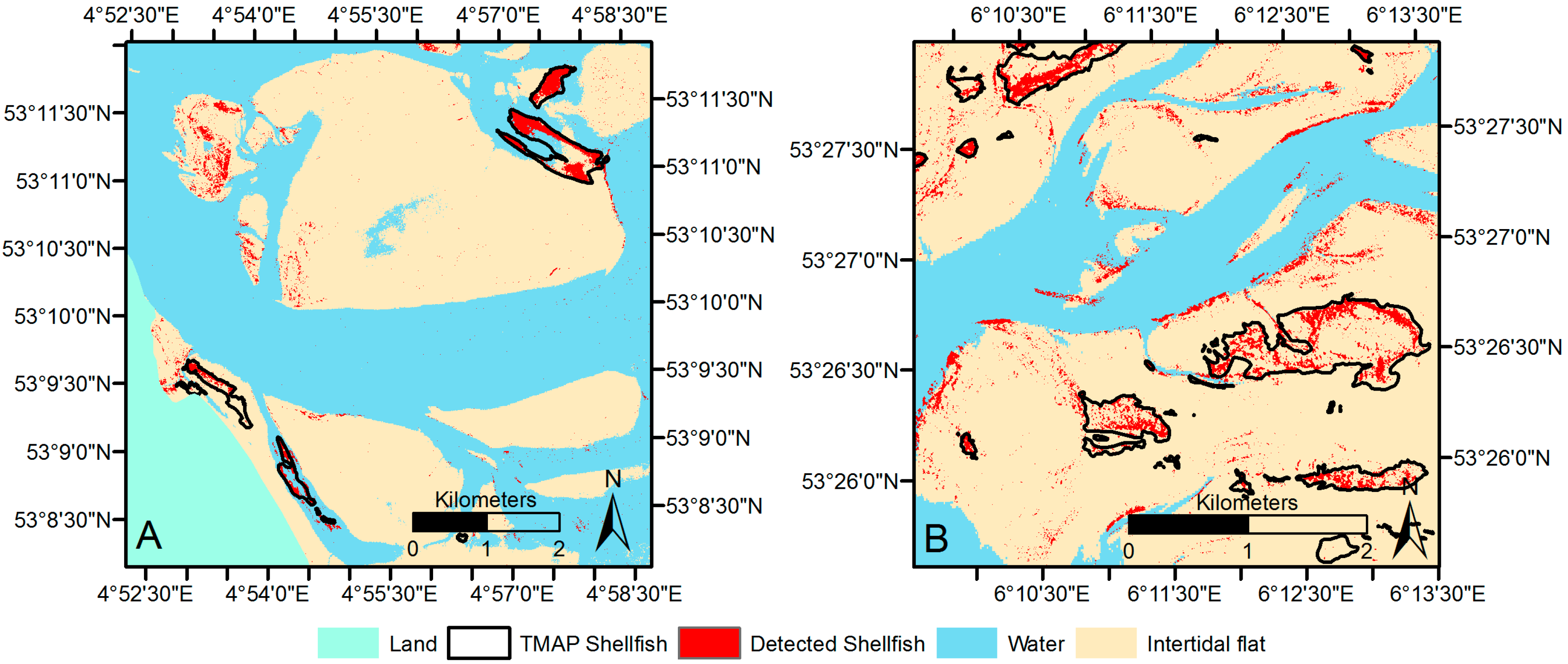
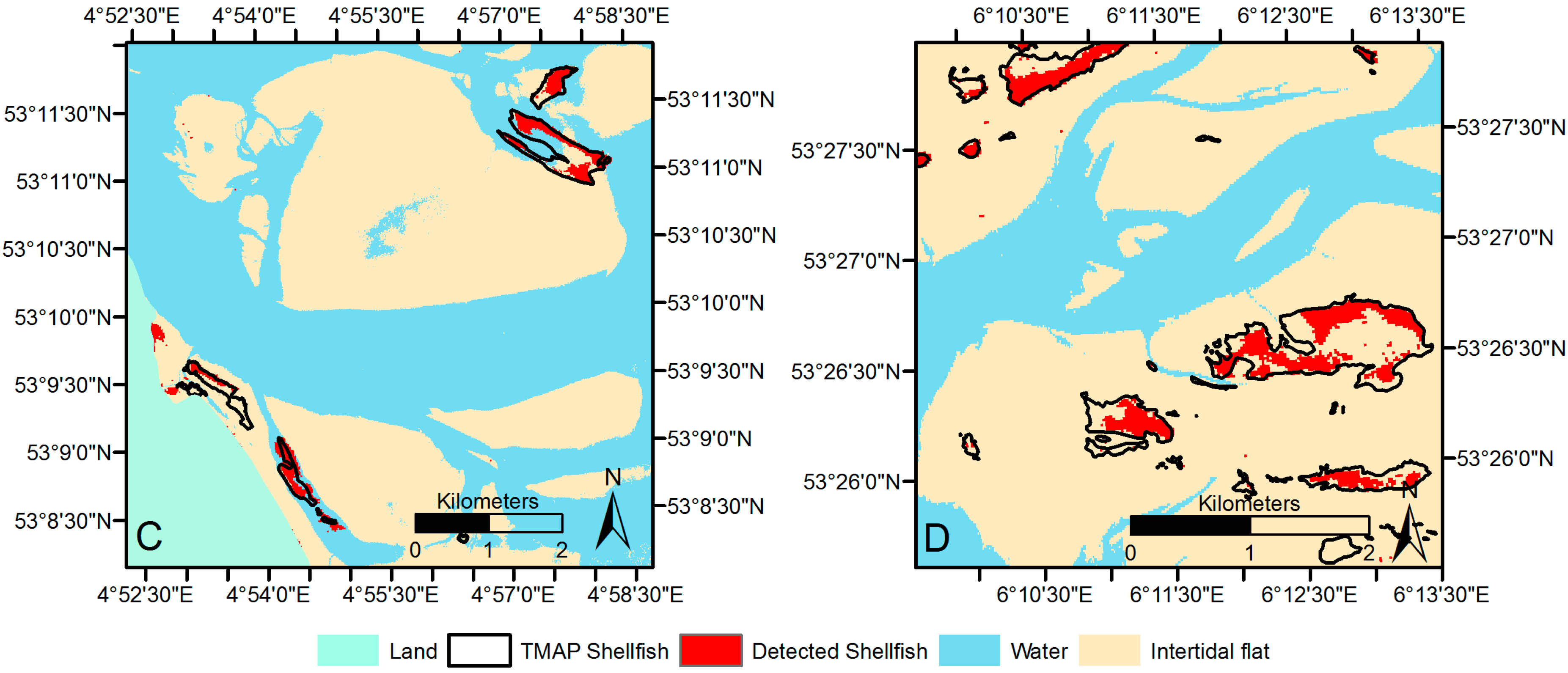
3.5. Comparing Shellfish Maps from SAR with Traditional Field Surveys

Table 5 displays how the SAR and TMAP shellfish maps compare to each other for the test areas in the Wadden Sea (Figure 1). Details of the classification results of dual polarized data along with TMAP shellfish outlines are depicted in Figure 10. The results show that SAR classification compares best to TMAP data if the classification is based on multivariate logistic regression incorporating information from both backscatter channels. Although X-band sensitivity seems most suitable for mapping shellfish as highlighted by Figure 6 and Figure 9, it appears that X-band is sensitive to strongly-rippled sediments and steep slopes (at the edges of gullies), which do cause strong backscatter, but do not depolarize the microwave signal. This causes many false positives in the dual-polarized classification scheme, because strongly-rippled sediments and slopes were not included in our field campaign. Because of this, the dual-polarized classifier causes misclassifications of sediments, which are high in VV, but low in VH. In fact, Table 5 shows that X-band classification can be improved if a double threshold is used (VV + VH). The dual-polarization classifier obtained from Radarsat-2’s C-band appears less sensitive to this. Furthermore, the classification results show that mapping using Radarsat-2’s C-band provides the most consistent agreement across sites, but clear differences in agreement between sites can be seen for TerraSAR-X, which agrees significantly more with the TMAP results in the western Wadden Sea (Texel) than in the eastern Wadden Sea (Schiermonnikoog). This could be explained by observations from the field that shellfish beds in the western part of the Wadden Sea are generally more strongly defined with clear boundaries, whereas in the eastern Wadden Sea, which is more shallow and sheltered, shellfish beds appear more dispersed with less clear boundaries. This would influence both the TMAP mapping and the SAR mapping, because the boundaries are harder to track in situ and the differences in backscatter between classes are less pronounced. The TMAP protocol also allows for misclassifications, and depending on the sensor resolution, this could result in worse performance of the mapping method. For instance, open patches can be mapped as shellfish beds, as long as they are less than 25 m wide. Furthermore, the monitoring is very time consuming, which means that it is impossible to map all of the beds each year; as a result, the data of some beds is copied from one year to the next if the bed appears to be unchanged after determination by an aerial survey. However, even small changes in bed size and shellfish densities could result in mismatches between the SAR and the TMAP data.

To further enhance shellfish mapping based on SAR data, we propose to use a texture method that uses the spatial information in the images. The signal generated by shellfish may not be stronger than the noise, which may cause elimination of parts of the shellfish beds during speckle filtering. Spatial information retrieved by methods, such as spatial autocorrelation or Haralick’s texture features, could help to enhance pixel-based image analysis [54]. Furthermore, since shellfish beds can be patchy in nature, this may have consequences for the classification of beds using high-resolution data. Methods that take into account the variation within classes in combination with the non-Gaussian behavior of SAR information prior to classification [55] may be beneficial to further enhance shellfish mapping using SAR.

4. Conclusions

Using data from a high number of ground stations, we were able to establish that dual-polarized X- and C-band SAR data can be used to distinguish between substrates with bare sediments with up to 5% shellfish cover (dispersed) and shellfish substrates (>5% cover). This observation was supported by the IEM and Oh’s model and highlights that SAR remote sensing is a valuable tool for shellfish monitoring. However, because the backscatter intensity saturates with relatively low RMSz values in shellfish beds, it is not possible to derive information on shellfish density or species composition. Mussels and oysters both increase RMSz of intertidal soft bottom substrates, with the largest RMSz values being found in oyster beds with high cover. Mussels, on the other hand, also increase RMSz, but at higher densities, the surfaces become smoother, as the mussels efficiently fill all available spots. No significant effects were found of the surface classes on correlation length.

Tide, weather and light conditions typically limit the window of opportunity to acquire data for optical remote sensing. SAR, on the other hand, only depends on suitable tidal conditions and much less on light and weather. Furthermore, SAR is less influenced by epibionts, which camouflage the shellfish in optical data. Furthermore, the application of single-acquisition SAR in epibenthic shellfish classification rather than multitemporal classification is particularly useful, because multitemporal data can now be used in change detection studies to monitor shellfish beds. These results highlight that by using SAR, monitoring surveys can be performed much more cost effectively and complement current field surveys. The current Radarsat-2, TerraSAR-X, CosmoSkyMed and Sentinel-1 missions provide suitable SAR data for such monitoring.

Table 5. Agreement between the SAR shellfish classification and the TMAP monitoring survey for the two sensors at Texel and Schiermonnikoog (see the text and Table 3 for an explanation).

	Texel								Schiermonnikoog
	TerraSAR-X				Radarsat-2				TerraSAR-X				Radarsat-2
	VV	VH	DUAL	VV + VH	HH	HV	DUAL	HH + HV	VV	VH	DUAL	VV + VH	HH	HV	DUAL	HH + HV
True Positives	64,873	77,090	68,992	60,275	962	1,115	1,100	899	125,729	105,155	122,806	80,792	1,709	2,774	2,607	1,567
True Negatives	12,644,700	12,098,222	12,690,954	12,761,094	214,337	216,287	216,314	216,645	13,833,734	14,387,332	14,218,344	14,491,808	242,406	245,140	245,276	245,820
False Positives	136,044	682,522	89,790	19,650	2694	744	717	386	696,931	143,333	312,321	38,857	4003	1269	1133	589
False Negatives	70,167	57,950	66,048	74,765	1339	1186	1201	1402	232,542	253,116	235,465	277,479	4371	3306	3473	4513
Sensitivity	0.48	0.57	0.51	0.45	0.42	0.48	0.48	0.39	0.35	0.29	0.34	0.23	0.28	0.46	0.43	0.26
Specificity	0.99	0.95	0.99	1.00	0.99	1.00	1.00	1.00	0.95	0.99	0.98	1.00	0.98	0.99	1.00	1.00
Precision	0.32	0.10	0.43	0.75	0.26	0.60	0.61	0.70	0.15	0.42	0.28	0.68	0.30	0.69	0.70	0.73
Accuracy	0.98	0.94	0.99	0.99	0.98	0.99	0.99	0.99	0.94	0.97	0.96	0.98	0.97	0.98	0.98	0.98
Kappa	0.38	0.16	0.46	0.56	0.31	0.53	0.53	0.50	0.19	0.33	0.29	0.33	0.27	0.54	0.52	0.37

Table 5. Agreement between the SAR shellfish classification and the TMAP monitoring survey for the two sensors at Texel and Schiermonnikoog (see the text and Table 3 for an explanation).

	Texel								Schiermonnikoog
	TerraSAR-X				Radarsat-2				TerraSAR-X				Radarsat-2
	VV	VH	DUAL	VV + VH	HH	HV	DUAL	HH + HV	VV	VH	DUAL	VV + VH	HH	HV	DUAL	HH + HV
True Positives	64,873	77,090	68,992	60,275	962	1,115	1,100	899	125,729	105,155	122,806	80,792	1,709	2,774	2,607	1,567
True Negatives	12,644,700	12,098,222	12,690,954	12,761,094	214,337	216,287	216,314	216,645	13,833,734	14,387,332	14,218,344	14,491,808	242,406	245,140	245,276	245,820
False Positives	136,044	682,522	89,790	19,650	2694	744	717	386	696,931	143,333	312,321	38,857	4003	1269	1133	589
False Negatives	70,167	57,950	66,048	74,765	1339	1186	1201	1402	232,542	253,116	235,465	277,479	4371	3306	3473	4513
Sensitivity	0.48	0.57	0.51	0.45	0.42	0.48	0.48	0.39	0.35	0.29	0.34	0.23	0.28	0.46	0.43	0.26
Specificity	0.99	0.95	0.99	1.00	0.99	1.00	1.00	1.00	0.95	0.99	0.98	1.00	0.98	0.99	1.00	1.00
Precision	0.32	0.10	0.43	0.75	0.26	0.60	0.61	0.70	0.15	0.42	0.28	0.68	0.30	0.69	0.70	0.73
Accuracy	0.98	0.94	0.99	0.99	0.98	0.99	0.99	0.99	0.94	0.97	0.96	0.98	0.97	0.98	0.98	0.98
Kappa	0.38	0.16	0.46	0.56	0.31	0.53	0.53	0.50	0.19	0.33	0.29	0.33	0.27	0.54	0.52	0.37

Figure 10. Details of the shellfish maps based on the TerraSAR-X classification for dual-polarization (brown) compared to the TMAP monitoring program (red). (a) TerraSAR-X classification of the western Wadden Sea (near Texel); (b) TerraSAR-X classification of the eastern Wadden Sea (near Schiermonnikoog); (c) Radarsat-2 classification of the western Wadden Sea; (d) Radarsat-2 classification of the eastern Wadden Sea.

Figure 10. Details of the shellfish maps based on the TerraSAR-X classification for dual-polarization (brown) compared to the TMAP monitoring program (red). (a) TerraSAR-X classification of the western Wadden Sea (near Texel); (b) TerraSAR-X classification of the eastern Wadden Sea (near Schiermonnikoog); (c) Radarsat-2 classification of the western Wadden Sea; (d) Radarsat-2 classification of the eastern Wadden Sea.

References

1. Heip, C.H.R.; Goosen, N.K.; Herman, P.M.J.; Kromkamp, J.; Middelburg, J.J.; Soetaert, K. Production and consumption of biological particles in temperate tidal estuaries. Oceanogr. Mar. Biol. 1995, 33, 1–149. [Google Scholar]
2. Albrecht, A. Soft bottom versus hard rock: Community ecology of macroalgae on intertidal mussel beds in the Wadden Sea. J. Exp. Mar. Biol. Ecol. 1998, 229, 85–109. [Google Scholar] [CrossRef]
3. Gutiérrez, J.; Jones, C.; Strayer, D.; Iribarne, O. Mollusks as ecosystem engineers: The role of shell production in aquatic habitats. Oikos 2003, 101, 79–90. [Google Scholar] [CrossRef]
4. Jones, C.G.; Gutiérrez, J.L.; Byers, J.E.; Crooks, J.A.; Lambrinos, J.G.; Talley, T.S. A framework for understanding physical ecosystem engineering by organisms. Oikos 2010, 119, 1862–1869. [Google Scholar] [CrossRef]
5. Van der Zee, E.M.; Heide, T.; Donadi, S.; Eklör, J.S.; Eriksson, B.K.; Olff, H.; Veer, H.W.; Piersma, T.; Zee, E.M. Spatially extended habitat modification by intertidal reef-building bivalves has implications for consumer-resource interactions. Ecosystems 2012, 15, 664–673. [Google Scholar]
6. Oliver, L.R.; Seed, R.; Reynolds, B. The effect of high flow events on mussels (Mytilus edulis) in the Conwy estuary, North Wales, UK. Hydrobiologia 2008, 606, 117–127. [Google Scholar] [CrossRef]
7. Beck, M.W.; Brumbaugh, R.D.; Airoldi, L.; Carranza, A.; Coen, L.D.; Crawford, C.; Defeo, O.; Edgar, G.J.; Hancock, B.; Kay, M. Shellfish Reefs at Risk: A Global Analysis of Problems and Solutions; The Nature Conservancy: Arlington, VA, USA, 2009; p. 52. [Google Scholar]
8. Troost, K. Causes and effects of a highly successful marine invasion: Case-study of the introduced Pacific oyster Crassostrea gigas in continental NW European estuaries. J. Sea Res. 2010, 64, 145–165. [Google Scholar] [CrossRef]
9. Kochmann, J.; Buschbaum, C.; Volkenborn, N.; Reise, K. Shift from native mussels to alien oysters: Differential effects of ecosystem engineers. J. Exp. Mar. Biol. Ecol. 2008, 364, 1–10. [Google Scholar] [CrossRef] [Green Version]
10. Markert, A.; Esser, W.; Frank, D.; Wehrmann, A.; Exo, K.-M. Habitat change by the formation of alien crassostrea-reefs in the Wadden Sea and its role as feeding sites for waterbirds. Estuar. Coast. Shelf Sci. 2013, 131, 41–51. [Google Scholar] [CrossRef]
11. Green, D.S.; Rocha, C.; Crowe, T.P. Effects of non-indigenous oysters on ecosystem processes vary with abundance and context. Ecosystems 2013, 16, 881–893. [Google Scholar] [CrossRef]
12. Nehls, G.; Witte, S.; Büttger, H.; Dankers, N.; Jansen, J.; Millat, G.; Herlyn, M.; Markert, A.; Kristensen, P.S.; Ruth, M.; et al. Beds of Blue Mussels and Pacific Oysters; Marencic, H., de Vlas, J., Eds.; Common Wadden Sea Secretariat, Trilateral Monitoring and Assessment Group: Wilhelmshaven, Germany, 2009. [Google Scholar]
13. De Vlas, J.; Brinkman, B.; Buschbaum, C.; Dankers, N.; Herlyn, M.; Kristensen, P.S.; Millat, G.; Nehls, G.; Ruth, M.; Steenbergen, J.; et al. Intertidal blue mussel beds. In Wadden Sea Quality Status Report 2004; Wadden Sea Ecosystem No. 19; Essink, K., Dettmann, C., Farke, H., Laursen, K., Lüerßen, G., Marencic, H., Wiersinga, W., Eds.; Common Wadden Sea Secretariat, Trilateral Monitoring and Assessment Group: Wilhelmshaven, Germany, 2005; pp. 190–200. [Google Scholar]
14. Van der Wal, D.; Herman, P.M.J.; Wielemaker-van den Dool, A. Characterisation of surface roughness and sediment texture of intertidal flats using ERS SAR imagery. Remote Sens. Environ. 2005, 98, 96–109. [Google Scholar] [CrossRef]
15. Choe, B.-H.; Kim, D.; Hwang, J.-H.; Oh, Y.; Moon, W.M. Detection of oyster habitat in tidal flats using multi-frequency polarimetric SAR data. Estuar. Coast. Shelf Sci. 2012, 97, 28–37. [Google Scholar] [CrossRef]
16. Dehouck, A.; Lafon, V.; Baghdadi, N.; Roubache, A.; Rabaute, T. Potential of TerraSAR-X imagery for mapping intertidal coastal wetlands. In Proceedings of the 4th TerraSAR-X Science Team Meeting, Oberpfaffenhofen, Germany, 14–16 February 2011.
17. Gade, M.; Melchionna, S.; Stelzer, K.; Kohlus, J. Multi-frequency SAR data help improving the monitoring of intertidal flats on the German North Sea coast. Estuar. Coast. Shelf Sci. 2014, 140, 32–42. [Google Scholar] [CrossRef]
18. Fung, A.K.; Li, Z.; Chen, K.S. Backscattering from a randomly rough dielectric surface. IEEE Trans. Geosci. Remote Sens. 1992, 30, 356–369. [Google Scholar] [CrossRef]
19. Oh, Y.; Sarabandi, K.; Ulaby, F. An empirical model and an inversion technique for radar scattering from bare soil surfaces. IEEE Trans. Geosci. Remote Sens. 1992, 30, 370–381. [Google Scholar] [CrossRef]
20. Dubois, P.C.; van Zyl, J.; Engman, T. Measuring soil moisture with imaging radars. IEEE Trans. Geosci. Remote Sens. 1995, 33, 915–926. [Google Scholar] [CrossRef]
21. Commito, J.; Rusignuolo, B. Structural complexity in mussel beds: The fractal geometry of surface topography. J. Exp. Mar. Biol. Ecol. 2000, 255, 133–152. [Google Scholar] [CrossRef] [PubMed]
22. Ens, B.J.; van Winden, E.A.J.; van Turnhout, C.A.M.; van Roomen, M.W.J.; Smit, C.J.; Jansen, J.M. Changes in the abundance of intertidal birds in the Dutch Wadden Sea in 1990–2008: Differences between East and West. Limosa 2009, 82, 100–112. [Google Scholar]
23. Lotze, H.K. Radical changes in the Wadden Sea fauna and flora over the last 2000 years. Helgol. Mar. Res. 2005, 59, 71–83. [Google Scholar] [CrossRef]
24. Reise, K.; Baptist, M.; Burbridge, P.; Dankers, N.; Fischer, L.; Flemming, B.; Oost, A.P.; Smit, C. The Wadden Sea—A Outstanding Tidal Wetland; Wadden Sea Ecosystem No. 29; Common Wadden Sea Secretariat: Wilhelmshaven, Germany, 2010; pp. 7–24. [Google Scholar]
25. Dankers, N.; Meijboom, A.; Cremer, J.S.M.; Dijkman, E.M.; Hermes, Y.; te Marvelde, L. Historische Ontwikkeling van Droogvallende Mosselbanken in de Nederlandse Waddenzee; Alterra-Rapport 876; Alterra: Wageningen, The Netherlands, 2003; p. 114. [Google Scholar]
26. Dankers, N.; Meijboom, A.; de Jong, M.; Dijkman, E.; Cremer, J.; van der Sluis, S. Het Ontstaan en Verdwijnen van Droogvallende Mosselbanken in de Nederlandse Waddenzee; Alterra-Rapport 921; Alterra: Wageningen, The Netherlands, 2004; p. 114. [Google Scholar]
27. Fey, F.; Dankers, N.; Steenbergen, J.; Goudswaard, K. Development and distribution of the non-indigenous Pacific oyster (Crassostrea gigas) in the Dutch Wadden Sea. Aquac. Int. 2009, 18, 45–59. [Google Scholar] [CrossRef]
28. Nienhuis, P.; Smaal, A. The Oosterschelde estuary, a case-study of a changing ecosystem: An introduction. Hydrobiologia 1994, 282/283, 1–14. [Google Scholar] [CrossRef]
29. Van Zanten, E.; Adriaanse, L. Verminderd Getij. Verkenning van mogelijke maatregelen om de erosie van platen, slikken en schorren van de Oosterschelde te beperken; Rapport RWS/2008; Rijkswaterstaat Zeeland: Middelburg, The Netherlands, 2008. [Google Scholar]
30. Radiometric calibration of TerraSAR-X data. 2008. Available online: http://www2.geo-airbusds.com/files/pmedia/public/r465_9_tsx-x-itd-tn-0049-radiometric_calculations_i3.00.pdf (accessed on 25 March 2015).
31. Lee, J.-S. Refined filtering of image noise using local statistics. Comput. Graph. Image Process. 1981, 15, 380–389. [Google Scholar] [CrossRef]
32. Wing, M. Consumer-grade GPS receiver measurement accuracy in varying forest conditions. Res. J. For. 2011, 5, 78–88. [Google Scholar]
33. Wu, C. VisualSFM: A Visual Structure from Motion System. Available online: http://ccwu.me/vsfm/ (accessed on 3 September 2012).
34. Ulaby, F.T.; Moore, R.K.; Fung, A.K. Microwave Remote Sensing, Active and Passive, Volume III: From Theory to Applications; Artech House: Dedham, MA, USA, 1986. [Google Scholar]
35. Petitpas, B.; Beaudoin, L.; Roux, M.; Rudent, J.-P. Roughness measurement from multi-stereo reconstruction. Int. Arch. Photogramm. Remote Sens. Spat. Inf. Sci. 2010, 38, Part 3B. 104–109. [Google Scholar]
36. R Core Team. R: A Language and Environment for Statistical Computing; R Foundation for Statistical Computing: Vienna, Austria, 2012. [Google Scholar]
37. Troost, K.; Drent, J.; Folmer, E.; van Stralen, M. Ontwikkeling van schelpdierbestanden op de droogvallende platen van de Waddenzee. De Levende Natuur 2012, 113, 83–88. [Google Scholar]
38. Gade, M.; Alpers, W.; Melsheimer, C.; Tanck, G. Classification of sediments on exposed tidal flats in the German Bight using multi-frequency radar data. Remote Sens. Environ. 2008, 112, 1603–1613. [Google Scholar] [CrossRef]
39. Lee, H.; Chae, H.; Cho, S.-J. Radar backscattering of intertidal mudflats observed by Radarsat-1 SAR images and ground-based scatterometer experiments. IEEE Trans. Geosci. Remote Sens. 2011, 49, 1701–1711. [Google Scholar] [CrossRef]
40. Park, S.-E.; Moon, W.M.; Kim, D. Estimation of surface roughness parameter in intertidal mudflat using airborne polarimetric SAR data. IEEE Trans. Geosci. Remote Sens. 2009, 47, 1022–1031. [Google Scholar] [CrossRef]
41. Fung, A.K.; Liu, W.Y.; Chen, K.S.; Tsay, M.K. An improved IEM model for bistatic scattering from rough surfaces. J. Electromagn. Waves Appl. 2002, 16, 689–702. [Google Scholar] [CrossRef]
42. Fung, A.K.; Chen, K.S. Microwave Scattering and Emission Models for Users; Artech House: Norwood, MA, USA, 2010; p. 430. [Google Scholar]
43. Hallikainen, M.; Ulaby, F.; Dobson, M.; El-rayes, M.; Wu, L. Microwave dielectric behavior of wet soil—Part 1: Empirical models and experimental observations. IEEE Trans. Geosci. Remote Sens. 1985, GE-23, 25–34. [Google Scholar] [CrossRef]
44. Oh, Y. Quantitative retrieval of soil moisture content and surface roughness from multipolarized radar observations of bare soil surfaces. EEE Trans. Geosci. Remote Sens. 2004, 42, 596–601. [Google Scholar] [CrossRef]
45. Fawcett, T. An introduction to ROC analysis. Pattern Recognit. Lett. 2006, 27, 861–874. [Google Scholar] [CrossRef]
46. Van den Ende, D.; Troost, K.; van Stralen, M.; van Zweeden, C.; van Asch, M. Het Mosselbestand en Het Areaal aan Mosselbanken op de Droogvallende Platen van de Waddenzee in Het Voorjaar van 2012; Wageningen IMARES Rapport, C149/12; IMARES: Yerseke, The Netherlands, 2012. [Google Scholar]
47. Davidson, M.W.J.; le Toan, T.; Mattia, F.; Satalino, G.; Maninnen, T.; Borgeaud, M. On the characterization of agricultural soil roughness for radar remote sensing studies. IEEE Trans. Geosci. Remote Sens. 2000, 38, 630–640. [Google Scholar] [CrossRef]
48. Verhoest, N.E.C.; Lievens, H.; Wagner, W.; Álvarez-Mozos, J.; Moran, M.S.; Mattia, F. On the soil roughness parameterization problem in soil moisture retrieval of bare surfaces from Synthetic Aperture Radar. Sensors 2008, 8, 4213–4248. [Google Scholar] [CrossRef]
49. Bretar, F.; Arab-Sedze, M.; Champion, J.; Pierrot-Deseilligny, M.; Heggy, E.; Jacquemoud, S. An advanced photogrammetric method to measure surface roughness: Application to volcanic terrains in the Piton de la Fournaise, Reunion Island. Remote Sens. Environ. 2013, 135, 1–11. [Google Scholar] [CrossRef]
50. Zribi, M.; Dechambre, M. A new empirical model to retrieve soil moisture and roughness from C-band radar data. Remote Sens. Environ. 2002, 84, 42–52. [Google Scholar] [CrossRef]
51. Van de Koppel, J.; Rietkerk, M.; Dankers, N.; Herman, P.M. Scale-dependent feedback and regular spatial patterns in young mussel beds. Am. Nat. 2005, 165, E66–E77. [Google Scholar] [CrossRef] [PubMed]
52. Kim, D.; Moon, W.M.; Kim, G.; Park, S.-E.; Lee, H. Submarine groundwater discharge in tidal flats revealed by space-borne synthetic aperture radar. Remote Sens. Environ. 2011, 115, 793–800. [Google Scholar] [CrossRef]
53. Landis, J.; Koch, G. The measurement of observer agreement for categorical data. Biometrics 1977, 33, 159–174. [Google Scholar] [CrossRef] [PubMed]
54. Haralick, R.M.; Shanmugam, K.; Dinstein, I. Textural features for image classification. IEEE Trans. Syst. Man Cybern. 1973, SMC-3, 610–621. [Google Scholar] [CrossRef]
55. Krylov, V.A.; Moser, G.; Serpico, S.B.; Zerubia, J. Supervised high-resolution dual-polarization SAR image classification by finite mixtures and copulas. IEEE J. Sel. Top. Signal Process. 2011, 5, 554–566. [Google Scholar] [CrossRef] [Green Version]