
Optimal Combination of Classification Algorithms and Feature Ranking Methods for Object-Based Classification of Submeter Resolution Z/I-Imaging DMC Imagery


Abstract
: Object-based image analysis allows several different features to be calculated for the resulting objects. However, a large number of features means longer computing times and might even result in a loss of classification accuracy. In this study, we use four feature ranking methods (maximum correlation, average correlation, Jeffries–Matusita distance and mean decrease in the Gini index) and five classification algorithms (linear discriminant analysis, naive Bayes, weighted k-nearest neighbors, support vector machines and random forest). The objective is to discover the optimal algorithm and feature subset to maximize accuracy when classifying a set of 1,076,937 objects, produced by the prior segmentation of a 0.45-m resolution multispectral image, with 356 features calculated on each object. The study area is both large (9070 ha) and diverse, which increases the possibility to generalize the results. The mean decrease in the Gini index was found to be the feature ranking method that provided highest accuracy for all of the classification algorithms. In addition, support vector machines and random forest obtained the highest accuracy in the classification, both using their default parameters. This is a useful result that could be taken into account in the processing of high-resolution images in large and diverse areas to obtain a land cover classification.1. Introduction
While the traditional pixel-based approach for remote sensing image classification is based on the statistical analysis of multispectral features of the pixels in an image, object-based image analysis (OBIA) allows the use of a wide range of additional information. The OBIA approach involves two steps: segmentation and classification. After segmentation, a very large number of features can be calculated for the resulting objects. The main advantages of OBIA, compared with pixel-based approaches, is the larger number of available features and the fact that the features convey more information when they are calculated on real objects than when sampled on a square grid. The availability of high spatial resolution satellites for civil use, for example QuickBird [1], and the release of eCognition in 2000, the first commercial OBIA software [2,3], are the two advances behind the expansion of OBIA.
eCognition [4] was initially developed by Definiens AG to overcome limitations in traditional approaches to the analysis of high spatial resolution remote sensing images and was the first commercial software that attempted to overcome such limitations. This software allows the extraction of objects from the image that have certain meaning and from which it is possible to extract certain semantics information. eCognition adopted an object-based and a multi-scale approach to the analysis of digital images and has become the most widely-used software in remote sensing when trying to extract thematic information from very high spatial resolution images. Its release has given universal access to tools that previously were only available in specialized research labs [2,3].
Until the mid-1990s, satellite imagery classification was mainly based on conventional statistical techniques, such as maximum likelihood or minimum distance, usually on a pixel basis. In recent years, due to the advances made in computing technology, alternative machine-learning algorithms have been proposed, particularly the use of artificial neural networks, weighted k-nearest neighbors (wk-NN), decision trees, support vector machines (SVM) and methods derived from the theory of fuzzy logic [5]. OBIA has not been unaffected by this trend, and several studies have used these algorithms to classify the objects produced by OBIA segmentation algorithms [6–16].
Whatever the algorithm used, having a very large number of features poses two problems. First, the larger the number of features used in classification, the longer the computing time needed. Second, using a very large number of explanatory features, especially when some of them are redundant, noisy or informationless, might result in a less accurate classification [17,18]. This is the so-called curse of dimensionality or the Hughes effect [19], which is an important issue in optimization and machine learning. Its main consequence is the need to greatly increase the amount of training objects necessary to maintain the sampling density in the space of features as the number of dimensions, i.e., the number of explanatory features, increases. This issue is increasing in importance due to the emergence of both OBIA and hyperspectral sensors. However, not all classification algorithms are sensitive to this effect. If no classification method is to be a priori discarded, it is better to use the lowest possible number of explanatory features.
However, it may be difficult to select the most relevant for classifying the objects. Thus, feature selection has become an important research topic in OBIA, and Lu and Weng [18] have identified the development of approaches to feature selection as one of the critical steps in remote sensing.
Despite its importance, it is not very common for OBIA-related papers to explicitly mention feature selection or the criteria and measurements used for the same. Most papers in which it is mentioned are based on Jeffries–Matusita distance [21–23], while others [10,15,24] use the Gini index, an index of the relative importance of features produced by algorithms based on decision trees. Laliberte et al. [25] compare the Jeffries–Matusita distance and the mean decrease in the Gini index (MDG) to select features to use with the wk-NN classification algorithm. MDG is a feature importance measurement provided by tree-based machine learning prediction methods, such as random forest. The use of Jeffries–Matusita distance assumes a normal multivariate distribution of the features in each of the classes. However, this assumption is not always met for features extracted from segmented objects. On the other hand, MDG is a non-parametric statistic that assumes no theoretical probability distribution, which, in principle, is a strength of MDG.
The main objectives of this research are:
To study the performance of four feature ranking methods to select the optimum feature subset to classify a very high resolution image using five classification algorithms.
To identify a feature ranking method that overcomes the Hughes effect in most of the classification methods.
To identify which of the analyzed classification algorithms is least sensitive to the Hughes effect.
Finally, to obtain a land cover layer.
To achieve these main objectives, it was necessary to fulfil three secondary objectives:
To generate a large number of potentially explanatory variables and to use them to evaluate several feature ranking and selection methods. The aim is to investigate whether these methods can identify those features that introduce redundant information or do not contribute to a statistical discrimination of classes.
To test a group of classification algorithms that represent the most important types of machine learning algorithms.
To implement a heuristic search process for feature selection. This will allow us to identify the feature subset that can achieve optimal classification.
The paper is organized as follows: In Section 2, we present the study area (Section 2.1) and the dataset, which is the result of applying multiresolution segmentation (Section 2.3) on a high-resolution multispectral image (Section 2.1). Several features obtained from this segmentation (Section 2.4) were used to classify the objects in order to test several classification algorithms (Section 2.5) and feature selection methods (Section 2.6). Different parameter values for the classification algorithms were also tested (Section 2.5). Special care was devoted to a sample design to obtain validation and calibration data (Section 2.2). In Section 3, we present the results, and finally, the conclusions are presented in Section 4.
2. Methods
The methodology of this research (summarized in Figure 1) comprises seven steps. Previous work with the image appears as Step 0 and is described in [26,27]. The aim of each step is:
To generate a large number of features (Section 2.4) calculated from the objects extracted in the image segmentation (Section 2.3).
To select an appropriate number of random validation areas and a set of training areas.
To apply four methods of feature ranking and selection (Section 2.6). The results of each of them are presented in Table 3 with features ordered according to each ranking method.
To execute several classification cycles (Section 2.6.2). For each classification algorithm (Section 2.5) and each vector of ranked features, a backward elimination process is executed until only two features remain. In each cycle, the kappa classification obtained from the validation data is stored. Thus, a vector with the values of the classification accuracy obtained for each of the 20 combinations of classification algorithms and ranking methods is obtained.
To display, using line graphs, how accuracy varies when the number of features increases by adding features in ranking order and how these variations differ among different classification algorithms (Section 3.2). For each combination of classification algorithm-ranking method, this display can identify the subset of variables that allows one to reach the maximum classification accuracy.
To modify some parameters of the classification algorithms identified in the literature as the most relevant to improve classification accuracy.
To analyze validation data using the best combination ranking method-classification algorithm.
Finally, a land cover layer is obtained.
2.1. Study Area and Data Used
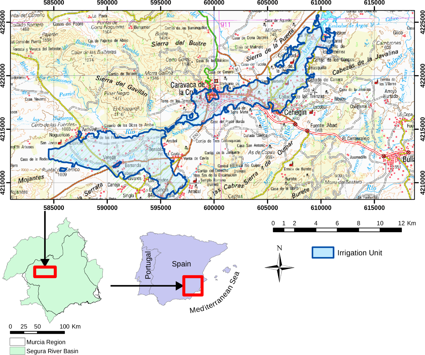
The study area (Figure 2) is located in the Murcia region (southeast Spain) and corresponds to Irrigation Unit (UDA) 28, as was defined in the Plan Hidrológico de la cuenca del Segura (River Segura Basin Hydrological Plan), the previously in-force water resources planning law passed on 24 July 1998 (R.D.1664/1998). A 150-m buffer zone has been added to ensure the complete inclusion of the relevant plots. The study area is large, 9070 ha, including the buffer, and includes different types of agricultural landscape; the intra-class variability of the Mediterranean countryside is also well represented.
This irrigation unit includes traditional orchards and modern, highly technical agriculture areas. As a result, there is a large variety of crops and land covers (40% grass and 60% trees). The traditional irrigation systems are very old. Initially, several springs in the limestone rocks, predominant in the River Argos headwaters, were exploited (more than 80% of the currently used resources). Later, several wells were excavated to complement those resources, and today, groundwater represents 15% of the resources used [32].
Most of the information used in this research was obtained from the Servicio de Integración y Gestión Ambiental (Environmental Integration and Management Service, SIGA), a branch of the Murcia regional government. The data, obtained under the Natmur-08 project [33], consist of a 2-m resolution multispectral (blue, green, red and near-infrared) image and a 0.45-m panchromatic digital image. The images corresponding to the study area were acquired on 9, 10 and 11 July 2008 with an Intergraph Z/I-Imaging Digital Mapping Camera. Both images were fused using Gram–Schmidt’s method [26,34,35] to obtain the final 0.45-m resolution multispectral image used in this study.
Additionally, digital terrain (DTM) and digital surface (DSM) models, with a resolution of 4 m, were used as ancillary data. These layers, also produced under the Natmur-08 project, had been interpolated from LiDAR point clouds obtained with a LEICA ALS50-III; we only had access to the interpolated layers and not to the original point clouds.
2.2. Classification Scheme, Sample Design and Field Data
As the aim of the work was to produce a map of agricultural land cover types, most of the classes included in the classification scheme have an agronomic sense. There are also two classes that include natural vegetation and artificial objects. The list of classes includes: Cereals (Cer); Rainfed arable lands (Rar); Rural wasteland (Rws); Irrigated grassland (Igr); Almond trees (Alm); Irrigated fruit trees (Ifr), including seedlings; Olive trees (Oli), including seedlings; Greenhouses (Gre); Other non-agricultural vegetation (Ot.Ve); and Other artificial areas (Ot.Ar).
Validation areas were sampled by generating random points; the plots (both agricultural and non-agricultural) where such points were located were selected as validation areas. Training areas were not randomly chosen; instead, those that adequately characterized the different classes were selected.
To obtain a statistically-consistent sampling strategy, the multinomial distribution equations [36] were used to calculate the sample size necessary for this research with a confidence level of 95% and a margin of error of 5%; the result was a total of 558 plots.
Two sampling schemes were used. The first random sampling included 254 validation areas, 200 of which correspond to agricultural uses. The main objective of this first sampling was to evaluate the spectral variability of each class. This information is useful to establish the sampling size of each stratum (land use class) in the second (stratified) sampling. The objective of this stratified sampling was to evaluate the accuracy of the classification by class rather than the accuracy of the whole scene.
One of the critical points of stratified sampling is the distribution of the samples across strata [37]. Some authors [36] claim that at least 50 samples for each class are needed in projects similar to ours.
In the present study, a minimum of 50 validation areas was used for each class. The other 58 were distributed proportionally to the spectral variability, calculated as a coefficient of variation, of the 10 classes. The distribution of sampling plots in each stratum is shown in Table 1.
The analysis unit, the unit on which the decision of the success or failure of the classification is made, is the object. Congalton and Green [36] recommend that the analysis unit is the object, even when the methodology is based on pixels. Objects have been used as analysis units in several studies [30,38–40].
All of the relevant objects in a validation area receive the label corresponding to the area. In areas with tree cover, almonds for instance, this label is manually assigned to all tree-objects or intersections of trees, the bare soil objects remaining unlabeled. In plots without trees, classless objects will be minimal. In this way, the labeled objects become the cases to classify.
Fieldwork was conducted in different periods: July 2009, and December 2010, to verify that land use had been correctly identified. Most of the plots were visited about a year after the capture of the images, so that the state of vegetation of image and fieldwork coincided. Table 1 also summarizes the distribution of the training and validation areas in the study area.
2.3. Image Segmentation
Multiresolution segmentation [41], the segmentation algorithm that we used with this image, is one of the most widely used in OBIA. It has been included in eCognition since the first versions [42,43], and despite its recent availability, it is rapidly becoming one of the most cited segmentation algorithms [18]. The details of the algorithm can be consulted in [41]. The key parameter for this segmentation method is the scale parameter, although there is no straightforward method available to obtain an optimum value of the same. The usual approach is to find a compromise value for the whole image by trying several values and evaluating the results [4,44–46]. However, this global approach needs a certain degree of uniformity in the image, so its application to large heterogeneous images, as in this study, may be difficult.
For this reason, a local approach for image segmentation, consisting of splitting the image into uniform spatial units, whereby the scale parameter is optimized locally, was assayed. The multiresolution segmentation algorithm was locally optimized with 3 spectral bands (red, green and near-infrared), all with the same importance. The importance of shape homogeneity was 30%, and the weighting coefficient for both compactness and smoothness was 50%. The importance given to each layer, the weights given to the form and the importance given to the compactness and smoothness were not optimized, but remained invariant throughout the whole optimization process. This methodology and the results are fully explained in [27]. As a result of the segmentation, a set of 1,076,937 objects was obtained.
2.4. Features Obtained from the Objects
Table 2 shows the object features calculated using eCognition software. Features are grouped into six main categories; their names are in bold face, and a short description is added when needed. Some of the features were only calculated with the red band. The reason for this is that, due to the high correlation within the visible spectrum, we did not think that blue and green bands would have added much to the discrimination capacity. Moreover, their inclusion would have strongly increased the computation complexity and would probably have complicated the feature selection process. The number of bands from which the features were calculated is indicated between parentheses. Technical details of every feature are described in DEFINIENS [47].
Texture is one of the most important features when identifying objects from a raster image. Haralick et al. [48] proposed a set of indices extracted from the grey level co-occurrence matrix (GLCM) [49,50]. The spatial relationships between neighboring pixels can be measured in each of the four main directions (N-S, NE-SW, E-W, SE-NW) or as a directionally-invariant average. Each textural feature is calculated in each of the four main directions in four layers—red band reflectivity, slope, aspect and convexity—and as a directionally-invariant average in the 10 input layers. Overall, there are 204 textural features.
The context features of objects are extracted by comparing an object feature (spectral, geometric or textural) with the same feature in the neighboring objects. These features can be used to improve the classification results [51]. Although the concepts of brighter and darker objects only make sense in features related to spectral properties and not in those related to topographical properties, we have maintained the feature names given by eCognition after the segmentation phase.
In summary, there are 40 spectral features, 5 pixel-based features, 24 geometric features, 204 texture features and 83 context features. This large number of features (356) poses a problem of collinearity that will be solved using the feature selection techniques introduced below.
2.5. Classification Algorithms
Five classification algorithms were used in this study, representing the most relevant approaches in remote sensing imagery classification: linear discriminant analysis [52] and naive Bayes [52], which are included among the classical parametric statistical techniques; weighted k-nearest neighbors [53], a method based on distances measured on the features space; random forest [5,54–61], which is a tree-based algorithm; and finally, support vector machines [5,61,62], which is a kernel-based algorithm.
Besides the features used for classification, other factors that might affect the accuracy of a classification algorithms are the values given to its parameters. To analyze this problem, the parameters of the classification algorithms identified as relevant in the literature were modified. Naive Bayes and linear discriminant analysis algorithms have no parameter to change.
Parameter changes were made sequentially, because complete modification was not feasible from a computational point of view. For example, with SVM, the optimal kernel was first determined using the default values for C and G. The C parameter was optimized using the optimal kernel and the default G. Finally, the G parameter was optimized using the optimal kernel and C value.
2.5.1. Linear Discriminant Analysis
Linear discriminant analysis is one of the first used, simplest and most used supervised classification algorithms. It tries to maximize the between-group variance and minimize the within-group variance, assuming that the features arise from a multivariate normal distribution with a class-specific mean vector and a common variance-covariance matrix [63].
The distributions of the predictors are first analyzed for each of the classes, and then, the Bayes theorem is used to obtain the probability of each class given the predictor values using the well-known Bayes equation:
The method receives its name from the fact that this equation is linear. Each observation X = x is finally assigned to the class k that maximizes Equation (2). In practice, linear discriminant analysis creates a linear frontier (hyperplane) between each pair of classes in the feature space and divides it into regions belonging to each class. The observations are classified according to the region in which they are located.
2.5.2. Naive Bayes
Bayesian networks model the dependence of the dependent variable on each of the predictors as a directed acyclic graph. The final node represents the dependent variable and the other nodes the predictors. The topology of the graph reflects the dependence relations among variables.
Naive Bayes [52] is the simplest case of a Bayesian network. In this case, just one arc goes from each of the predictors to the dependent variable. This means that predictors are assumed to be conditionally independent in every class. Therefore, a simplified version of the Bayesian equation is applied. The function to maximize is:
Although conditional independence is a rather strong assumption, naive Bayes is a competitive algorithm whose results can even outperform other algorithms [64–66]. Another advantage is that the independence assumption causes a significant reduction in computing time [66].
2.5.3. Weighted k-Nearest Neighbors
When used for classification, k-nearest neighbors [53] estimates the class for every new observation using the k-closest observations, according to a distance metric, from the training set. Class probabilities for the new observation are estimated as the proportion of training set neighbors in each class. Ties are broken randomly or by including the k + 1 closest neighbor in the calculation.
An important parameter to be taken into account is k, the number of neighbors. A small value leads to a low-bias, high-variance prediction, increasing the probability of over-fitting, while too large a value cause a high-bias classification.
Despite its simplicity, this algorithm has been successful in a large number of classification problems [61].
The algorithm wk-NN is a modification of k-NN, in which each training example is weighted according to its distance from the point being classified.
As regards the wk-NN parameters, both the number of neighboring cases taken into account to predict and the distance measurement can be modified. Euclidean and Manhattan are the available distance measurements, the latter being the default option. Although it is possible to vary the type of kernel, it was not modified, following the advice of the author of the R package that implements the algorithm [53]. For modifying the number of neighbors, an arithmetic progression from 1 to 19, with a step of two, was tested.
2.5.4. Random Forest
Decision trees build a classification model by a recursive binary partition of a labeled dataset into increasingly homogeneous nodes. Homogeneity is measured by the Gini index [54], defined as:
Random forest [56] generates a large number of unpruned trees (500–2,000) using a bootstrapped sample of the cases; each node division is carried out with a randomized subset of the predictors to add randomness and to decrease the correlation between trees. Uncorrelation is a desirable property in ensemble learning classifiers because the different results give sense to the voting system that is finally used to estimate the class to which any new case belongs. Random forest can outperform other machine learning classification algorithms (support vector machines or neural networks) and other decision tree algorithms [56,57].
As the classification errors of any tree are diluted into the ensemble, random forest does not over-fit the model to the dataset [6,56,67,68]. Since the cases not included in a bootstrapped sample are not used to fit the corresponding tree, they can be used to perform a cross-validation accuracy estimation [60].
The number of trees and the number of predictors used to train each tree are the parameters that can be set by the user. Nevertheless, the method does not seem to be very sensitive to these values, which are, by default, 500 and the square root of the number of available features [57,59]. In general, random forests do remarkably well and require very little tuning [61].
A disadvantage of random forest compared with the simple classification tree approach is that, as individual trees cannot be examined separately, it becomes a “black box” approach [68]. However, it provides several metrics that help to interpret the model. Variable importance is evaluated by calculating how the accuracy or the Gini index would decrease if the data for that predictor were permuted randomly. The resulting values can be used to compare the relative importance among predictor variables. In this way, the result is easier to interpret than in other algorithms, such as neural networks [68].
The most relevant parameters in random forest are the number of trees (ntree) generated and the number of randomly chosen features used to divide the nodes in each of the individual trees (mtry). The default values in the R package randomForest are ntree = 500 and mtry = int( ), where Nf is the number of features. Random forest does not seem to be very sensitive to its parameters [57,61]; however, we then tried using ntree = {250, 500, 1000} and doubling and halving mtry following the recommendations of the authors of the package [57].
2.5.5. Support Vector Machines
Support vector machines (SVM) [61,62] are a very flexible classification algorithm that tries to maximize the distance between the hyperplanes that separate classes and the cases closer to those hyperplanes, the so-called support vectors. These large distances, margins in SVM terminology, give SVM a greater generalization capacity, because they maximize the probability of correctly classifying new cases located in the area between two different classes.
The decision function used to estimate the class of each new case is:
SVM is included in the category of kernel methods; the function K(xi, u) is the kernel function. In the simplest case, it is just the dot product of both feature vectors, producing linear hyperplanes. In addition, different non-linear kernel functions can be used to transform the space of features and, in this way, produce non-linear hyperplanes.
When the classes are not completely separable, a cost parameter will penalize those cases situated on the wrong side of the separating hyperplane. The higher the cost, the most complex the hyperplane needed to avoid misclassifications. Therefore, a higher cost parameter will also produce a model with a lower generalization capacity.
SVM is conceived of as an algorithm to separate two classes. When there are more than two classes, it is usually applied on a one vs. the others basis, using the distance to the separating hyperplanes as a membership criterion.
In the case of SVM, it is possible to modify the kernel type, the cost parameter C and the width parameter G. Four kernel transformations were tested: linear, polynomial, radial and sigmoidal. For the penalty parameter, the following values were tested:
1 being the default value. For the width parameter, the following values were tested:
2.5.6. Software Used
R software [69], an open source statistical program and language, was used to run all classification algorithms. The classification algorithms used in this work are included in the packages: randomForest [57], e1071 [70], kknn [71] and MASS [72].
2.6. Feature Ranking and Selection Methods
A successful approach in machine learning is to view feature selection as a heuristic procedure in which a subset of possible features is specified at each step of an iterative search [73]. Such a procedure involves 3 steps:
Ranking all features in accordance with a criterion related to their relevance to classify the dataset.
Iteratively improving a classification model by adding features according to their rank.
Selecting the best feature subset according to a classification accuracy measurement.
2.6.1. Feature Ranking
Four feature ranking criteria were used: average correlation, maximum correlation, Jeffries–Matusita distance and mean decrease in the Gini index. In addition to these four ranking methods, a random ranking was used to compare the results.
Average correlation is a simple approach, in which the relevance of a feature is related to its correlation with other features. Thus, highly-correlated variables will be considered as redundant information, since they only contribute to classification complexity without adding greater discrimination power. The correlation matrix (using the Pearson correlation coefficient in this case) is used to calculate the importance of any feature as its average correlation coefficient. After eliminating the feature with the highest average correlation, the correlation matrix is recalculated, and the procedure continues. The feature eliminated in each iteration is stored, and finally, a vector of features in ascending order of importance is obtained.
Maximum correlation is very similar to the above criterion; the only difference being that the criterion for choosing the feature to be deleted in each cycle is the maximum rather than the average correlation.
The Jeffries–Matusita distance between each pair of classes measures a feature’s average capacity to separate classes. Features are ranked according to this distance, whose equation is:
The mean decrease in Gini index is a feature importance statistic produced by random forest averaging Gini indices of the individual trees [54]. The importance of a variable in a tree is measured as the sum of the decrements in the Gini index attributed to that feature. The global feature importance is the average of its importance for all of the trees.
The mean decrease in the Gini index ranking method is obtained by running as many classification cycles as there are features available. In each cycle, MDG is calculated, and the feature with the lowest MDG value is eliminated from the dataset. Thus, the order in which each feature is removed gives a rank of its importance.
2.6.2. Iterative Classification and Accuracy Criterion
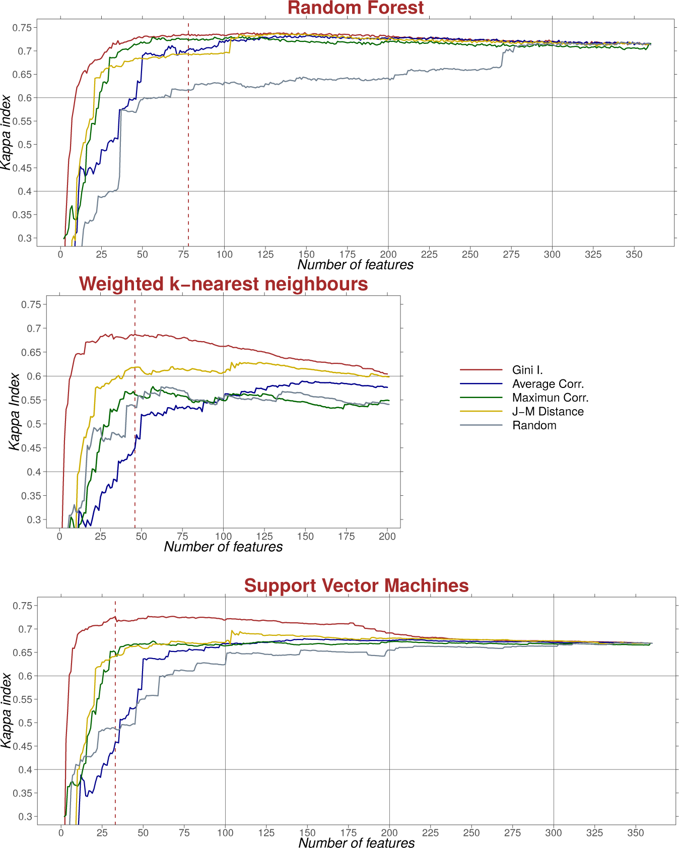
For each classification algorithm and feature ranking method, all of the features were used to train the algorithm; the kappa index [36] was then calculated from the validation sample, and the least important feature was eliminated from the dataset. This procedure was repeated until only one feature was left. A line graph for each classification method was then drawn in a graph whose horizontal axis is the number of features used in each cycle and where the ordinate is the kappa value obtained (Figures 3 and 4). A visual analysis of the curves was sufficient to locate the number of features that maximizes accuracy.
Because wk-NN classification is substantially slower than the others, only 199 classification cycles were run using the 200 most important features. Linear discriminant analysis and naive Bayes only use quantitative features, which means 333 features and, accordingly, 332 classification steps. Random forest and SVM were classified with the complete dataset of 356 features. Because all of these classification cycles were replicated for the five ranking methods (including the random ranking), the total number of classification was 7865.
3. Results
3.1. Feature Selection
Tables 3 and 4 summarize the results of the feature ranking process. Table 3 shows the 40 most important features according to each ranking method, while Table 4 shows the kind of features included in different subsets: the 40 most important features according to each ranking method, that is, a summary of Table 3, and the optimal subsets using MDG in each of the classification algorithms.
The features calculated within the objects seem to be the most relevant, especially in the case of the MDG ranking method. Geometry features do not appear among the 40 most important features for MDG; textural features do not appear among the 40 most important according to the Jeffries–Matusita distance ranking method; finally, border features do not appear within the subsets obtained using the correlation methods. Although these results are interesting and should be analyzed in the future, it is not the objective of this study to enter into these details.
The features selected using the average correlation method do not include any spectral variable, only three features related with skewness and one related with IHS transformation. Most of the features drawn by this method are related to shape, context and texture.
On the other hand, the methods based on Jeffries–Matusita distance and MDG included several pairs of closely-correlated features in the first rankings. This was expected in the case of Jeffries–Matusita distance, because if a feature provides large separability, all of the features correlated with it will show similar separability.
3.2. Classification
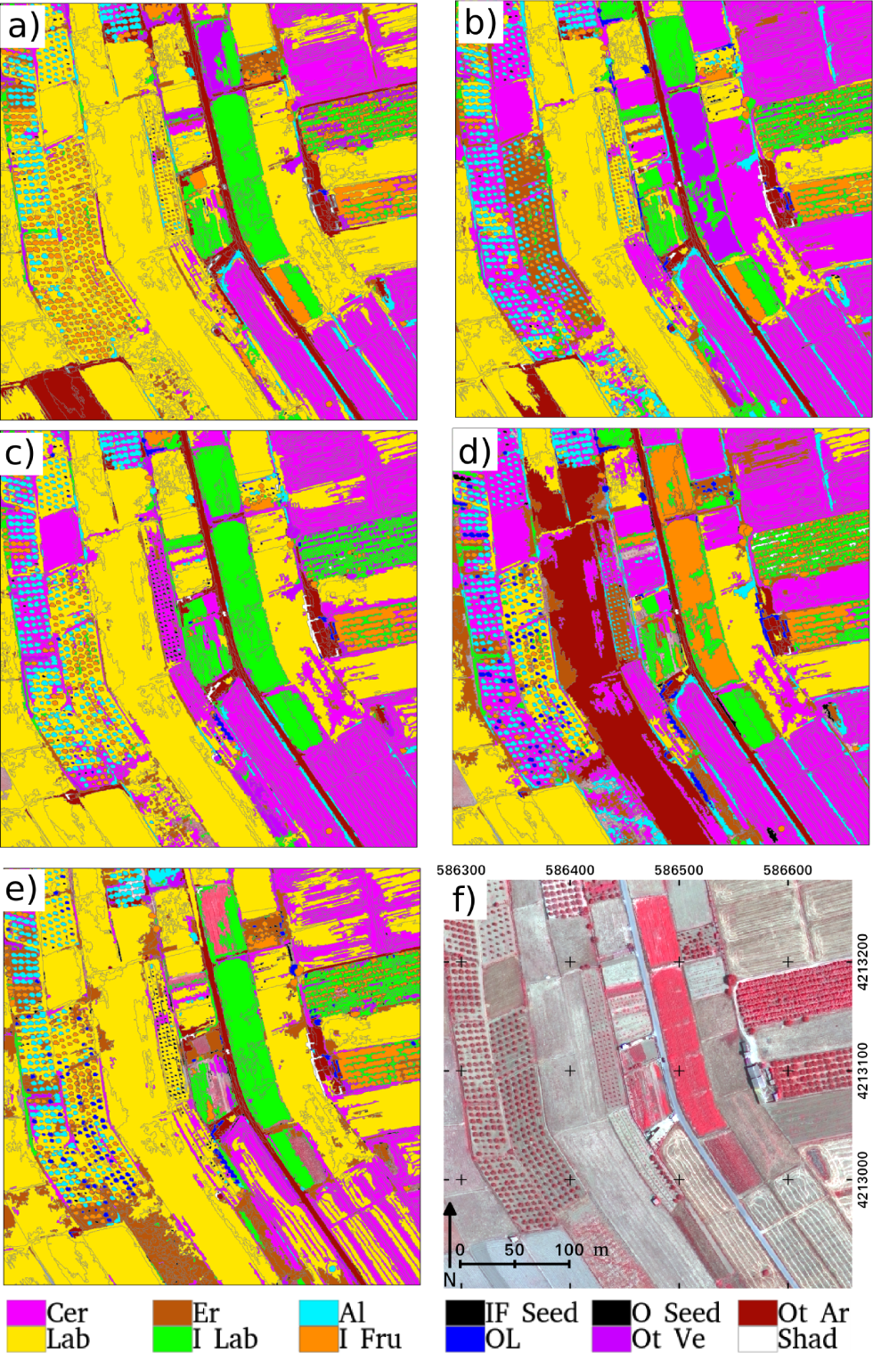
The kappa statistic is calculated from a set of confusion matrices with 14 classes. These classes include the original classification scheme, but with adult trees separated from seedlings in irrigated fruit trees and olive trees and mature irrigated grassland separated from plants in an early state of development. The final new classification scheme also includes shadows (Shd) cast by objects in the validation areas (usually trees and buildings).
Figures 3 and 4 show the result of the kappa index in several classification cycles using every ranking method and classification algorithm. These figures should be read from right to left, since a backward elimination was performed.
The random forest classification method provided the highest accuracy, especially using the features ranked by the MDG index. Figure 3 shows no significant changes until the curve reaches the 50th feature, meaning that random forest is quite insensitive to the presence of redundant or noisy features, i.e., to the Hughes effect. This is because random forest does not overfit the model to the calibration data.
Another ranking method that attains high accuracy with random forest is maximum correlation; however, with fewer than 75 features, the results are inferior to those obtained with MDG, especially when fewer than 30 features are used. Using about 50 features, the kappa indices of MDG and maximum correlation are virtually the same. Furthermore, the downward slope of the kappa index between 50 and 10 is greater in the maximum correlation method than in MDG.
The average correlation gives very similar values to the previous two methods when more than 140 features are used, while if fewer features are included, there is a substantial decrease in accuracy. As expected, the worst results were obtained when features were ranked randomly.
MDG also reaches a high accuracy value when using the wk-NN classification algorithm. A kappa value of 0.69 is reached with 46 features, which can be considered the most appropriate number of features to be used with wk-NN. This classification method is, however, more sensitive to the presence of unnecessary features. Using the first 200 features, the kappa index is about 0.60, which is significantly different compared with the value obtained with the first 40 features. According to these data, this classification algorithm seems to be more sensitive to the Hughes effect than random forest. If wk-NN is the only algorithm to be used for classification, a major effort in feature selection will be needed.
When using the Jeffries–Matusita distance, a kappa value of only 0.60 is reached in the best case. Moreover, the curve does not show any increase in accuracy when the least important features are eliminated. The maximum correlation results are also rather weak, below 0.55; however, this ranking method seems to be able to remove unnecessary features in some sections of the curve, such as the stretch between 85 and 50 features, in which there is an increase in accuracy. Whatever the case, this method cannot be considered to provide acceptable results. Average correlation also gives very poor results; analyzing the form of the curve, it seems that important features are eliminated, and, as a result, dimensionality reduction provides no increase in accuracy.
When analyzing SVM, the highest kappa index is obtained with MDG and 29 features. The sensitivity to high dimensionality is not very great, although it is greater than in the case of random forest. In the case of MDG, the kappa index remains stable between 360 and 200 features, while from 200 to 125 features, it increases and remains stable until 30 features are reached, when there is a sharp drop. The rest of the ranking methods have much lower kappa values. The curves obtained from maximum correlation and Jeffries–Matusita distance are very similar, while the average correlation curve is quite different.
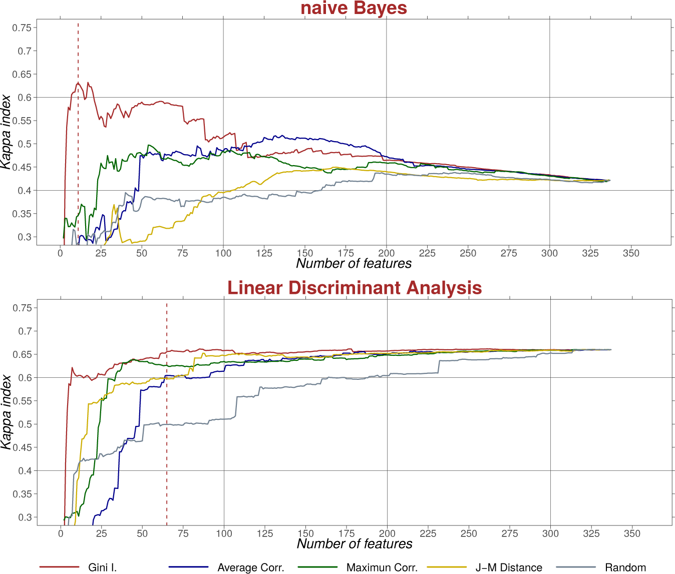
With naive Bayes, again, MDG provides the highest accuracy, although its highest kappa value is 0.63, well below that reached by random forest or SVM. However, this accuracy peak is reached with only 11 features, creating quite a parsimonious model. It is very sensitive to the Hughes effect: with 337 features, the kappa values are very low, around 0.4. In the case of MDG, the kappa index increases steadily as features are eliminated, and there are several points on the graph where the elimination of only one or two features causes a particularly sharp increase in classification accuracy. The other methods provide very weak results in all cases, with kappa values under 0.5 throughout the curve.
The general performance of linear discriminant analysis is much lower than that of random forest, wk-NN and SVM. This algorithm, too, obtains the best results with MDG; although, in this case, there are fewer differences with the other ranking methods, especially average separability. The number of features in the optimal subset with MDG (65) is much higher than in the case of naive Bayes. The curve remains almost stable until the 90th feature, when there is a slight increase in accuracy. It is below the 50th feature that accuracy rates begin to fall very sharply.
Table 5 summarizes the confusion matrices of the five classification methods using the MDG ranking method (always the one that provides maximum accuracy) and the feature set that produced the greatest accuracy. The table shows omission and commission errors in each class, kappa, accuracy and the number of features required to reach the maximum kappa index. Both random forest and SVM produced the best result, the former being slightly better. SVM needed fewer features than random forest to reach the maximum accuracy; however, Figure 3 shows that random forest results have a large sill, which means that even with substantially fewer features, accuracy is almost the maximum possible. Interestingly, naive Bayes reaches its maximum accuracy with just 11 features, although its kappa and accuracy are much smaller than those corresponding to random forest and SVM.
As regards parameter optimization, except for the number of neighbors in the wk-NN algorithm, modifying the default parameters brings about only small improvements in accuracy. In the case of wk-NN, the use of the Euclidean distance rather than Manhattan distance produced a substantial decrease in accuracy. Accuracy increases as does the number of neighbors, reaching a peak with 19. More neighbors were not tested, because the increase from k = 17 to k = 19 was very modest, and using k = 19 and Manhattan distance led to a kappa value of 0.69.
As an example, Figure 5 shows a subset of the results obtained by each classification method, using in each case the proposed optimal feature set.
4. Discussion
Laliberte et al. [25] compare the Jeffries–Matusita distance and MDG to select features for use with the wk-NN classification algorithm. Although both ranking methods, along with the other two, were used in our research, the results are not completely comparable, because in the above-mentioned work, the number of features to be selected was fixed a priori, whereas in our study, the optimal number of variables to be used in each algorithm was one of the outcomes of the ranking and selection process. While the results of the cited work suggest that the results obtained with the Gini index are very similar to those obtained with the Jeffries–Matusita distance, the results obtained in this study lead to a different conclusion: that better results are obtained using the MDG ranking method whichever classification algorithms is tested.
Pal [6], Duro et al. [10], Löw et al. [15] and Ghosh and Joshi [16] obtained similar results to us. In our study, SVM needed fewer features than random forest to reach the maximum accuracy, as was observed by Ghosh and Joshi [16]. In our work, as occurred in Löw et al. [15], using SVM to classify with the whole feature set produces a higher error than when using the optimal subset in accordance with the MDG ranking method. The classification results of Pal [6] are very similar to those obtained in the present work. By contrast, Ghosh and Joshi [16] found that SVM performed better than random forest, with a difference in favor of the first of 0.05 in kappa. Since the difference was slight, bearing in mind that both studies are quite comparable, we can conclude that, in terms of classification accuracy, both algorithms provide very similar results. Interestingly, naive Bayes reaches its maximum accuracy with just 11 features, although its kappa and accuracy are much smaller than those corresponding to random forest and SVM.
As regards parameter optimization, except for the number of neighbors in the wk-NN algorithm, modifying the default parameters brings about only small improvements in accuracy. In the case of wk-NN, the use of Euclidean distance rather than Manhattan distance led to a substantial decrease in accuracy. More neighbors were not tested because the increase from k = 17 to k = 19 was very modest and using k = 19 and Manhattan distance gave a kappa value of 0.69.
We agree with Pal [6] that the need for only two parameters to be set and the lack of sensitivity to these parameters are clear advantages of using random forest. For example, no important effect was observed when the number of trees was doubled or halved compared with the default value. Similar results were obtained when modifying the mtry parameter. In this respect, our empirical results also coincide with those given by Duro et al. [10].
Another advantage of random forest is that, along with linear discriminant analysis, it is insensitive to the Hughes effect. In the case of random forest, similar results were found by Duro et al. [10]. However, other authors, like Guan et al. [11], obtained different results. In this work, decreasing from 48 to 10 features led to a significant improvement in classification accuracy (from kappa = 0.6 to kappa = 0.8). We think that the cause of these differences is two-fold: first, the study areas in [11] are very small; second, the ntree parameter in [11] was 100, quite lower that the recommended value that we used in our study (500). SVM has low sensitivity to the Hughes effect, while wk-NN and, especially, naive Bayes are very sensitive.
5. Conclusions
Regarding the classification algorithms, random forest and SVM have provided the highest classification accuracy, followed by wk-NN. On the other hand, the results of naive Bayes and linear discriminant analysis are less accurate, with kappa indices around 10 percentage points lower than those obtained with random forest or SVM.
It was to be expected that the MDG feature ranking method would obtain a good result with random forest, because both methods are fairly closely related. However, MDG obtained the highest accuracy with all classification algorithms. This consistency strongly suggests that MDG can be considered as one of the best options for ranking features.
Another advantage of random forest is that, along with linear discriminant analysis, it is insensitive to the Hughes effect. SVM has low sensitivity, while wk-NN and, especially, naive Bayes are very sensitive.
Random forest and SVM obtain the highest accuracy with the default parameters, which is an advantage over other classification methods, such as wk-NN, which need to be calibrated. In fact, the accuracy obtained with wk-NN increased with the number of neighbor cases used to classify. However, this increase in accuracy was still small.
According to Laliberte et al. [25], because our comparison of feature selection methods was based on the same segmentation, it was reasonable to assume that the classification accuracies could be attributed to the feature selection methods and not to the prior segmentation step.
In summary, random forest with features selected using MDG was the most suitable algorithm for classifying the analyzed image. If only one classification method is used, it should be random forest, because it provides the greatest accuracy values and does not really need feature selection, unless the number of features available is too large for the computing power available.
The results also allowed an improvement in land use classification, which was the main objective of analyzing this image.
Object-oriented analysis represents an advantage over the pixel-based approach because of the substantial reduction in the number of cases. Segmentation can be regarded as a necessary step for remote sensing imagery classification when using cutting-edge machine learning techniques with large computing requirements. We agree with Ghosh and Joshi [16] when they say that “The extensive use of open source R statistical software allows free and easy access of the framework under study to researchers and users across the world.”
Acknowledgments
This study was carried out within the framework of 15233/PI/10, funded by Fundación Séneca. We would like to thank the CARM Environmental Integration and Management Service (SIGA) for providing us with the imagery of our study area. We also thank the three anonymous reviewers whose suggestions have substantially improved this manuscript.
Author Contributions
Both authors contributed equally in the design of the research. Fulgencio Cánovas-García did the field work, identifying training and validation areas. Both authors contributed equally to the programming of R scripts. Francisco Alonso-Sarría reviewed and edited the final version of the manuscript. Finally, both authors have read and accepted the final version of the manuscript.
Conflicts of Interest
The authors declare no conflict of interest.
References
- Aplin, P.; Atkinson, P.; Curran, P. Fine spatial resolution satellite sensors for the next decade. Int. J. Remote Sens. 1997, 18, 3873–3881. [Google Scholar]
- Castilla, G.; Hay, G. Image objects and geographic objects. In Object-Based Image Analysis. Spatial Concepts for Knowledge-Driven Remote Sensing Applications; Blaschke, T., Lang, S., Hay, G., Eds.; Springer: Berlin, Germany, 2008; pp. 91–110. [Google Scholar]
- Blaschke, T. Object based image analysis for remote sensing. ISPRS J. Photogramm. Remote Sens. 2010, 65, 2–16. [Google Scholar]
- Gao, H. Digital Analysis of Remotely Sensed Imagery; McGraw-Hill: New York, NY, USA, 2009. [Google Scholar]
- Tso, B.; Mather, P. Classification Methods for Remotely Sensed Data, 2nd ed.; Taylor & Francis: Boca Raton, FL, USA, 2009. [Google Scholar]
- Pal, M. Random forest classifier for remote sensing classification. Int. J. Remote Sens. 2005, 26, 217–222. [Google Scholar]
- Tzotsos, A.; Argialas, D. Support Vector Machine classification for Object-Based Image Analysis. In Object-Based Image Analysis. Spatial Concepts for Knowledge-Driven Remote Sensing Applications; Blaschke, T., Lang, S., Hay, G., Eds.; Springer: Berlin, Germany, 2008; pp. 663–677. [Google Scholar]
- Mallinis, G.; Koutsias, N.; Tsakiri-Strati, M.; Karteris, M. Object-based classification using Quickbird imagery for delineating forest vegetation polygons in a Mediterranean test site. ISPRS J. Photogramm. Remote Sens. 2008, 63, 237–250. [Google Scholar]
- Ok, A.O.; Akar, O.; Gungor, O. Evaluation of random forest method for agricultural crop classification. Eur. J. Remote Sens. 2012, 45, 421–432. [Google Scholar]
- Duro, D.C.; Franklin, S.E.; Dubé, M.G. Multi-scale object-based image analysis and feature selection of multi-sensor earth observation imagery using random forests. Int. J. Remote Sens. 2012, 33, 4502–4526. [Google Scholar]
- Guan, H.; Li, J.; Chapman, M.; Deng, F.; Ji, Z.; Yang, X. Integration of orthoimagery and lidar data for object-based urban thematic mapping using random forests. Int. J. Remote Sens. 2013, 34, 5166–5186. [Google Scholar]
- Aguilar, M.; Saldaña, M.; Aguilar, F. GeoEye-1 and WorldView-2 pan-sharpened imagery for object-based classification in urban environments. Int. J. Remote Sens. 2013, 34, 2583–2606. [Google Scholar]
- Fan, H. Land-cover mapping in the Nujiang Grand Canyon: integrating spectral, textural, and topographic data in a random forest classifier. Int. J. Remote Sens. 2013, 34, 7545–7567. [Google Scholar]
- Abdel-Rahman, E.M.; Ahmed, F.B.; Ismail, R. Random forest regression and spectral band selection for estimating sugarcane leaf nitrogen concentration using EO-1 Hyperion hyperspectral data. Int. J. Remote Sens. 2013, 34, 712–728. [Google Scholar]
- Löw, F.; Michel, U.; Dech, S.; Conrad, C. Impact of feature selection on the accuracy and spatial uncertainty of per-field crop classification using Support Vector Machines. ISPRS J. Photogramm. Remote Sens. 2013, 85, 102–119. [Google Scholar]
- Ghosh, A.; Joshi, P. A comparison of selected classification algorithms for mapping bamboo patches in lower Gangetic plains using very high resolution WorldView 2 imagery. Int. J. Appl. Earth Obs. Geoinf. 2014, 26, 298–311. [Google Scholar]
- Landgrebe, D.A. Signal Theory Methods in Multispectral Remote Sensing; Wiley: Hoboken, NJ, USA, 2003. [Google Scholar]
- Lu, D.; Weng, Q. A survey of image classification methods and techniques for improving classification performance. Int. J. Remote Sens. 2007, 28, 823–870. [Google Scholar]
- Hughes, G. On the mean accuracy of statistical pattern recognizerss. IEEE Trans. Inf. Theory. 1968, 14, 55–63. [Google Scholar]
- Oommen, T.; Misra, D.; Twarakav, N.; Prakash, A.; Sahoo, B.; Bandopadhyay, S. An objective analysis of support vector machine based classification for remote sensing. Math. Geosci. 2008, 40, 409–424. [Google Scholar]
- Marpu, P.; Niemeyer, I.; Nussbaum, S.; Gloaguen, R. A procedure for automatic object-based classification. In Object-Based Image Analysis. Spatial Concepts for Knowledge-Driven Remote Sensing Applications; Blaschke, T., Lang, S., Hay, G., Eds.; Springer: Berlin, Germany, 2008; pp. 169–184. [Google Scholar]
- Carleer, A.; Wolff, E. Urban land cover multi-level region-based classification of VHR data by selecting relevant features. Int. J. Remote Sens. 2006, 27, 1035–1051. [Google Scholar]
- Nussbaum, S.; Menz, G. Object-Based Image Analysis and Treaty Verification; Springer: Berlin, Germany, 2008. [Google Scholar]
- Yu, Q.; Gong, P.; Clinton, N.; Biging, G.; Kelly, M.; Schirokauer, D. Object-based Detailed Vegetation Classification with Airborne High Spatial Resolution Remote Sensing Imagery. Photogramm. Eng. Remote Sens. 2006, 72, 799–811. [Google Scholar]
- Laliberte, A.; Browning, D.; Rango, A. A comparison of three feature selection methods for object-based classification of sub-decimeter resolution UltraCam-L imagery. Int. J. Appl. Earth Obs. Geoinf. 2012, 15, 70–78. [Google Scholar]
- Cánovas-García, F.; Alonso-Sarría, F. Comparación de técnicas de fusión en imágenes de alta resolución espacial. Geofocus 2014, 14, 144–162. [Google Scholar]
- Cánovas-García, F.; Alonso-Sarría, F. A local approach to optimise the scale parameter in Multiresolution Segmentation for multispectral imagery. Geocarto Int. 2015. [Google Scholar] [CrossRef]
- Lucieer, A.; Stein, A. Existential uncertainty of spatial objects segmented from satellite sensor imagery. IEEE Trans. Geosci. Remote Sens. 2002, 40, 2518–2521. [Google Scholar]
- Neubert, M.; Meinel, G. Evaluation of Segmentation Programs for High Resolution Remote Sensing Applications, Procedings of the Joint ISPRS/EARSeL Workshop “High Resolution Mapping from Space 2003”, Hannover, Germany, 6–8 October 2003.
- Liua, D.; Xiab, F. Assessing object-based classification: Advantages and limitations. Remote Sens. Lett. 2010, 1, 187–194. [Google Scholar]
- Johnson, B.; Xie, Z. Unsupervised image segmentation evaluation and refinement using a multi-scale approach. ISPRS J. Photogramm. Remote Sens. 2011, 66, 473–483. [Google Scholar]
- Confederación Hidrográfica del Segura. Plan Hidrológico de la cuenca del Segura; Technical Report, 1998. Available online: https://www.chsegura.es/chs/planificacionydma/plandecuenca/documentoscompletos/ accessed on 15 April 2015.
- CARM. Proyecto NATMUR-08: Vuelo fotogramétrico y levantamiento LiDAR de la Región de Murcia, Available online: http://www.murcianatural.carm.es/natmur08/ accessed on 15 April 2015.
- Farebrother, R. Algorithm AS 79: Gram-Schmidt Regression. J. R. Stat. Soc. Ser. C 1974, 23, 470–476. [Google Scholar]
- Clayton, D. Algorithm AS 46: Gram-Schmidt Orthogonalization. J. R. Stat. Soc. Ser. C 1971, 20, 335–338. [Google Scholar]
- Congalton, R.; Green, K. Assessing the Accuracy of Remotely Sensed Data. Principles and Practices, 2nd ed.; CRC Press: Boca Raton, FL, USA, 2008. [Google Scholar]
- Clairin, R.; Brion, P. Manual de muestreo; Cuadernos de Estadística, La Muralla y Hespérides: Madrid, Spain, 2001. [Google Scholar]
- Greinier, M.; Labrecque, M; Beniot, M.; Allard, M. Accuracy Assessment Method for Wetland Object-Based Classification. In GEOBIA 2008—Pixels, Objets, Intelligence. Geographic Object Based Image Analysis for the 21 Century; Hay, G., Blashke, T., Marceau, D., Eds.; International Society for Photogrammetry and Remote Sensing: Hannover, Germany, 2008; Volume XXXVIII-4-C1. [Google Scholar]
- Su, W.; Li, J.; Chen, Y.; Liu, Z.; Zhang, J.; Lou, T.; Suppiah, I.; Hashim, S.; Atikah, M. Textural and local spatial statistic for the object-oriented classification of urban areas using hight resolution imagery. Int. J. Remote Sens. 2008, 29, 3105–3117. [Google Scholar]
- Yu, Q.; Gong, P.; Tian, Y.; Pu, R.; Yang, J. Factors affecting spatial variation of classification uncertainty in an image object-based vegetation mapping. Photogramm. Eng. Remote Sens. 2008, 74, 1007–1018. [Google Scholar]
- Baatz, M.; Schape, A. Multi-resolution segmentation: An optimization approach for high quality multi-scale image segmentation. In Angewandte Geographische Informationsverarbeitung XIII; Strobl, J., Blaschke, T., Griesebner, G., Eds.; Wichmann Verlag: Heidelberg, Germany, 2000; pp. 12–23. [Google Scholar]
- Lucieer, A. Uncertainties in Segmentation and Their Visualisation. Ph.D. Thesis, Universiteit Utrecht, Utrecht, The Netherlands, 2004. [Google Scholar]
- Benz, U.; Hofmann, P.; Willhauck, G.; Lingenfelder, I.; Heynen, M. Multi-resolution, object-oriented fuzzy analysis of remote sensing data for GIS-ready information. ISPRS J. Photogramm. Remote Sens. 2004, 58, 239–258. [Google Scholar]
- Platt, R.; Rapoza, L. An evaluation of an object-oriented paradigm for land use/land cover classification. Prof. Geogr. 2008, 60, 87–100. [Google Scholar]
- Tzotsos, A.; Iosifidis, C.; Argialas, D. A hybrid texture-based and region-based multi-scale image segmentation algorithm. In Object-Based Image Analysis. Spatial Concepts for Knowledge-Driven Remote Sensing Applications; Blaschke, T., Lang, S., Hay, G., Eds.; Springer: Berlin, Germany, 2008; pp. 221–236. [Google Scholar]
- Conrad, C.; Fritsch, S.; Zeidler, J.; Rücker, G.; Dech, S. Per-Field irrigated crop classification in arid central Asia using SPOT and ASTER data. Remote Sens 2010, 2, 1035–1056. [Google Scholar]
- DEFINIENS, eCognition Developer 8. Reference Book; DEFINIENS: München, Germany, 2009.
- Haralick, R.; Shanmugan, K.; Dinstein, I. Textural features for image classification. IEEE Trans. Syst. Man Cybern. 1973, SMC-3, 610–621. [Google Scholar]
- DEFINIENS, Definiens Developer 7. Reference Book; DEFINIENS: München, Germany, 2008.
- Recio Recio, J. Técnicas de extraccién de características y clasificación de imágenes orientada a objetos aplicadas a la actualización de bases de datos de ocupación del suelo. Ph.D. Thesis, Universidad Politécnica de Valencia, Valencia, Spain, 2009. [Google Scholar]
- Marpu, P. Geographic Object-Based Image Analysis. Ph.D. Thesis, Techniche Universität Bergakademie Freiberg, Freiberg, Germany, 2009. [Google Scholar]
- Mitchell, T. Machine Learning; McGraw-Hill: Boston, FL, USA, 1997. [Google Scholar]
- Schliep, H. Weighted k-Nearest-Neighbor Techniques and Ordinal Classification; Paper 399; Institut für Statistik der Ludwig-Maximilians-Universität München: Munich, Germany, 2004. [Google Scholar]
- Breiman, L.; Friedman, J.; Stone, C.; Olshen, R. Classification and Regression Trees; Chapman and Hall/CRC: London, UK, 1984. [Google Scholar]
- Breiman, L. Bagging predictors. Mach. Learn. 1996, 24, 123–140. [Google Scholar]
- Breiman, L. Random forest. Mach. Learn. 2001, 45, 5–32. [Google Scholar]
- Liaw, A.; Wiener, M. Classification and regression by random forest. R News. 2002, 2, 18–22. [Google Scholar]
- Timofeev, R. Classification and Regression Trees (CART) Theory and Applications. Master’s Thesis, Humboldt University, Berlin, Germany, 2004. [Google Scholar]
- Gislason, P.; Benediktsson, L.; Sveinsson, J. Random forests for land cover classification. Pattern Recognit. Lett. 2006, 27, 294–300. [Google Scholar]
- Cutler, D.; Edwards, T.; Beard, K.; Cutler, A.; Hess, K.; Gibson, J.; Lawler, J. Random forest for classification in ecology. Ecology 2007, 88, 2783–2792. [Google Scholar]
- Hastie, T.; Tibshirani, R.; Friedman, J. The Elements of Statistical Learning: Data Mining, Inference, and Prediction, 2nd ed.; Springer: Berlin, Germany, 2009. [Google Scholar]
- Camps-Valls, G.; Bruzzone, L. Kernel Methods for Remote Sensing Data Analysis; Wiley: Hoboken, NJ, USA, 2009. [Google Scholar]
- James, G.; Witten, D.; Hastie, T.; Tibshirani, R. An Introduction to Statistical Learning: With Applications in R (SpringerTexts in Statistics); Springer: Berlin, Germany, 2013. [Google Scholar]
- Rish, I. An empirical study of the Naive Bayes classifier, Proceedings of IJCAI 2001 Workshop on Empirical Methods in Artificial Intelligence, Seattle, WA, USA, 4 August 2001; pp. 41–46.
- Zhang, H. The optimality of Naive Bayes, Proceedings of Seventeenth International Florida Artificial Intelligence Research Society Conference, Florida, FL, USA, 12–14 May 2004.
- Kuhn, M.; Johnson, K. Applied Predictive Modeling; Springer: Berlin, Germany, 2013; p. 574. [Google Scholar]
- Guhimre, B.; Rogan, J.; Miller, J. Contextual land-cover classification: Incorporating spatial dependence in land-cover classification models using random forests and the Getis statistic. Remote Sens. Lett. 2010, 1, 45–54. [Google Scholar]
- Prasad, A.M.; Iverson, L.; Liaw, A. Newer classification and regression tree techniques: Bagging and random forests for ecological prediction. Ecosystems 2006, 9, 181–199. [Google Scholar]
- R Development Core Team, R: A language and Environment for Statistical Computing; R Foundation for Statistical Computing: Vienna, Austria, 2009; p. 409.
- Meyer, D.; Dimitriadou, E.; Hornik, K.; Weingessel, A.; Leisch, F. e1071: Misc Functions of the Department of Statistics (e1071), TU Wien, 2014. Available online: http://cran.rproject.org/web/packages/e1071/ accessed on 15 April 2015.
- Schliep, K.; Hechenbichler, K. kknn: Weighted k-Nearest Neighbors, Available online: http://cran.rproject.org/web/packages/kknn/ accessed on 15 April 2015.
- Venables, W.N.; Ripley, B.D. Modern Applied Statistics with S, 4th ed.; Springer: New York, NY, USA, 2002. [Google Scholar]
- Blum, A.; Langley, P. Selection of relevant features and examples in machine learning. Artif. Intell. 1997, 97, 245–271. [Google Scholar]


| Classes | Training | Validation | |||||
|---|---|---|---|---|---|---|---|
| Plots | Objects | % Area | Plots | Objects | % Area | CV | |
| Cer | 30 | 830 | 0.07 | 53 | 1043 | 0.21 | 0.14 |
| Rar | 55 | 1399 | 0.32 | 54 | 1459 | 0.90 | 0.19 |
| Rws | 31 | 1309 | 0.10 | 55 | 1567 | 0.52 | 0.21 |
| Igr | 37 | 1187 | 0.07 | 55 | 3920 | 0.57 | 0.21 |
| Alm | 32 | 4080 | 0.07 | 55 | 8289 | 0.14 | 0.23 |
| Ifr | 63 | 5617 | 0.18 | 58 | 4894 | 0.29 | 0.35 |
| Oli | 39 | 2987 | 0.05 | 58 | 4613 | 0.19 | 0.33 |
| Gee | 38 | 341 | 0.03 | 55 | 1290 | 0.10 | 0.20 |
| Ot.Ve | – | 2307 | 0.18 | 56 | 3885 | 0.26 | 0.25 |
| Ot.Ar | – | 4687 | 0.40 | 59 | 7396 | 0.86 | 0.41 |
| Total | 325 | 24,744 | 1.46 | 558 | 38,356 | 4.048 | – |
| Original bands | Pixels within the objects | ||
|---|---|---|---|
| B1 | red | MEAN(10) | |
| B2 | green | SD (10) | standard deviation |
| B3 | blue | MAX(1) | maximum value |
| B4 | near-infrared | MIN(1) | minimum value |
| C5 | DTM | ASYM(10) | skewness |
| C6 | DSM | INTENSITY(1) | |
| C7 | DSM-DTM | HUE(1) | |
| C8 | slope | SATURATION(1) | |
| C9 | aspect | NDVI (1) | |
| C10 | convexity | RATIO(4) | percentage of total bleftness |
| Object geometry | Object texture | ||
| PERIM (1) | including inner borders | GLCM.homo (26) | homogeneity |
| LENGTH (1) | GLCM.cont (26) | contrast | |
| WIDTH (1) | GLCM.dis (26) | dissimilarity | |
| L/W (1) | LENGTH/WIDTH | GLCM.ent (26) | entropy |
| ASYM02 (1) | asymmetry | GLCM.asm (26) | angular second moment |
| BORDER.i (1) | PERIM/perimeterSR | GLCM.mean (26) | mean |
| COMPACT (1) | LENGT H · WIDTH/AREA | GLCM.sd (26) | standard deviation |
| DENSITY (1) | similarity to a square | GLCM.corr (26) | correlation |
| ELLIPTIC.fit (1) | similarity to a ellipse | Object border | |
| MAIN.dir, (1) | main direction | MEAN.int.bor (1) | mean reflectivity of the inner border |
| RADIUS.largest (1) | radius of the largest enclosed ellipse | MEAN.ext.bor (1) | mean reflectivity of the outer border |
| RADIUS.smallest (1) | radius of the smallest enclosed ellipse | BOR.cont (1) | difference between MEAN.int.bor and the borders of the surrounding objects |
| RECT.fit (1) | similarity to a rectangle | SD.rec (1) | standard deviation of pixels not in the object but in the SR |
| ROUNDNESS (1) | NEIGH.cont (1) | difference between MEAN and the mean of pixels not in the object but in the surrounding rectangle | |
| SHAPE.i (1) | PERIM/(4 ·) | Object context | |
| AREA.excl (1) | area excluding inner polygons | NUM.c (1) | number of neighboring objects |
| AREA.incl (1) | area including inner polygons | MEAN.c (2) | neighboring objects’ mean |
| LENGTH.arc (1) | average length of arcs | MEAN.d.c (10) | mean difference to neighboring objects, using objects’ means |
| LONGEST.arc (1) | length of longest arc | MEAN.d.c.dr (10) | mean difference to darker neighboring objects |
| COMPACT.p (1) | AREA divided by the area of a circle with the same perimeter | MEAN.d.c.dr2 (10) | modified mean difference to darker neighboring objects when the darker object is being analyzed |
| NUMBER.arcs (1) | MEAN.d.c.br (10) | mean difference to blefter neighboring objects | |
| NUMBER.int (1) | number of inner objects | MEAN.d.c.br2 (10) | modified mean difference to blefter neighboring objects when the blefter object is being analyzed |
| PERIMETER.p (1) | excluding inner borders | NUM.dr (10) | number of darker neighboring objects |
| SD.edges (1) | standard deviation of length of arcs | NUM.br (10) | number of blefter neighboring objects |
| POR.bor.br (10) | relative border to blefter neighboring objects |
| Average Cor. | Maximum Cor. | Jeffries-Matusita Distance | Gini Index | |
|---|---|---|---|---|
| 1 | AREA | NDVI | AREA.incl | MEAN:C5 |
| 2 | MAIN.dir | NUM.c | AREA.excl | MEAN:C6 |
| 3 | POR.bor.br:C5 | GLCM.homo:C5 (Dis) | MEAN:C7 | NDVI |
| 4 | POR.bor.br:C8 | MAIN.dir | NUM.dr:B1 | NEIGH.c:B1 |
| 5 | GLCM.homo:C8 (N) | ASYM:C5 | NUM.dr:B2 | RATIO:B3 |
| 6 | ASYM:B4 | MEAN.d.c:C5 | NUM.dr:B3 | RATIO:B4 |
| 7 | MEAN.d.c.dr:C7 | ASYM:C8 | MEAN:B1 | MEAN:C8 |
| 8 | ASYM:C5 | MEAN.d.c:C8 | NUM.dr:B4 | MEAN.d.c:B1 |
| 9 | MEAN.d.c.br:B2 | ASYM:C10 | MIN:B1 | MEAN:B2 |
| 10 | SATURATION | ASYM:C9 | PERIMETER | SD:C6 |
| 11 | GLCM.homo:C9 (E) | GLCM.corr:B1 (NE) | INTENSITY | RATIO:B1 |
| 12 | ASYM:C10 | POR.bor.br:C7 | MEAN:B2 | RATIO:B2 |
| 13 | MEAN.d.c:C8 | L/W | HUE | MEAN.d.c.dr:B1 |
| 14 | MEAN.d.c.br2:C9 | MEAN.d.c:C10 | MEAN.int.bor:B1 | MEAN:B4 |
| 15 | L/W | SD:C9 | MEAN.d.c.dr:C7 | MEAN.d.c:B3 |
| 16 | POR.bor.br:C10 | MEAN:C7 | MEAN.d.c.dr2:C7 | HUE |
| 17 | ASYM:C9 | ASYM:C7 | POR.bor.br:B2 | GLCM.asm:B1 (SE) |
| 18 | GLCM.cont:C7 (Dis) | ASYM:B1 | RATIO:B4 | MEAN.d.c.br:B1 |
| 19 | MEAN.d.c:C10 | MEAN:B4 | NUMBER.arcs | RATIO:B1 |
| 20 | MEAN.d.c.br:C7 | GLCM.cont:C5 (Dis) | POR.bor.br:B1 | MEAN.d.c.dr:B4 |
| 21 | ASYM:C8 | MEAN.d.c:C9 | POR.bor.br:B3 | SD:C5 |
| 22 | MEAN.d.c.dr2:C9 | SATURATION | NEIGH.cont:B1 | MEAN:B1 |
| 23 | SD:B3 | MEAN.c:C10 | PERIMETER.p | INTENSITY |
| 24 | MEAN.d.c:C8 | MEAN:C8 | NDVI | MEAN.d.c:B2 |
| 25 | GLCM.sd:C8 (SE) | COMPACT | RATIO:B1 | SATURATION |
| 26 | ASYM:C7 | SD:B1 | MEAN.d.c.br:C7 | SD:C7 |
| 27 | MEAN.d.c.dr2:C5 | GLCM.corr:C8 (N) | SD:C7 | MEAN.d.c.dr:B3 |
| 28 | ASYM:B3 | MEAN.d.c:C8 | MEAN:B3 | MIN:B1 |
| 29 | POR.bor.br:C9 | MEAN.d.c.dr:C5 | MEAN.d.c:C7 | GLCM.corr:B3 (Dis) |
| 30 | POR.bor.br:C7 | MEAN:C5 | RATIO:B2 | SD.rec:B1 |
| 31 | GLCM.corr:B1(SE) | MEAN.d.c.br:C5 | MEAN.d.c.br2:C7 | MEAN.ext.bor:B1 |
| 32 | MEAN.d.c:C10 | SD.rec:B1 | NUM.c | MEAN.d.c.br:C7 |
| 33 | GLCM.homo:C8 (E) | SD:C8 | MEAN.ext.bor:B1 | GLCM.ent:B1 (SE) |
| 34 | MEAN:C6 | GLCM.sd:C10 (Dis) | WIDTH | MEAN.d.c:C8 |
| 35 | GLCM.homo:C9 (N) | BOR.cont:B1 | SD:C6 | MEAN:C7 |
| 36 | ASYM02 | GLCM.homo:C7 (Dis) | POR.bor.br:B4 | MEAN.d.c:B4 |
| 37 | NUMBER.int | GLCM.homo:B1 (Dis) | RATIO:B3 | MEAN.d.c.dr:B2 |
| 38 | MEAN.d.c.br2:C5 | GLCM.corr:B1 (SE) | MEAN.d.c.dr2:B2 | MEAN.d.c.br:B2 |
| 39 | ASYM:C6 | RATIO:B3 | MEAN.d.c.dr2:B3 | MEAN.int.bor:B1 |
| 40 | GLCM.med:B1 (E) | LENGTH.arc | MEAN.d.c.dr2:B1 | GLCM.corr:B1 (E) |
| Feature Subset | Within Object | Geometry | Textural | Border | Context |
|---|---|---|---|---|---|
| Maximum correlation (40) | 16 | 5 | 8 | 0 | 11 |
| 40 | 12.5 | 20 | 0 | 27.5 | |
| 36.4 | 20.8 | 3.8 | 0 | 13.2 | |
| Average correlation (40) | 12 | 4 | 8 | 0 | 16 |
| 30 | 10 | 20 | 0 | 40 | |
| 27.3 | 16.7 | 3.8 | 0 | 19.3 | |
| Separability (40) | 14 | 7 | 0 | 3 | 16 |
| 35 | 17.5 | 0 | 7.5 | 40 | |
| 31.8 | 29.2 | 0 | 60 | 19.3 | |
| MDG (40) | 21 | 0 | 4 | 3 | 12 |
| 52.5 | 0 | 10 | 7.5 | 30 | |
| 47.7 | 0 | 1.9 | 60 | 14.5 | |
| Random forest optimal (50) | 22 | 1 | 7 | 4 | 16 |
| 44 | 2 | 14 | 8 | 32 | |
| 50 | 4.2 | 3.4 | 80 | 19.3 | |
| wk-nearest neighbors (46) optimal | 22 | 1 | 5 | 3 | 15 |
| 47.87 | 2.2 | 10.9 | 6.5 | 32.6 | |
| 50 | 4.2 | 2.4 | 60 | 18.1 | |
| Support vector machines (29) optimal | 20 | 0 | 2 | 1 | 6 |
| 69 | 0 | 6.9 | 3.5 | 20.7 | |
| 45.5 | 0 | 1 | 20 | 7.2 | |
| Naive Bayes optimal (11) | 10 | 0 | 0 | 1 | 0 |
| 90.9 | 0 | 0 | 9.1 | 0 | |
| 22.7 | 0 | 0 | 20 | 0 | |
| LDA optimal (90) | 30 | 7 | 22 | 4 | 27 |
| 33.3 | 7.8 | 24.4 | 4.4 | 30 | |
| 68.2 | 29.2 | 10.6 | 80 | 32.5 | |
| OE | Cer | Rar | Rws | Igr | Alm | Ifr | Oli | Gre | Ot.Ve | Ot.Ar | Shd | K | F | Size |
|---|---|---|---|---|---|---|---|---|---|---|---|---|---|---|
| RF | 0.28 | 0.43 | 0.64 | 0.37 | 0.09 | 0.34 | 0.29 | 0.18 | 0.10 | 0.06 | 0.37 | 0.74 | 0.78 | 78 |
| wk-NN | 0.35 | 0.43 | 0.55 | 0.34 | 0.10 | 0.27 | 0.44 | 0.12 | 0.23 | 0.14 | 0.45 | 0.70 | 0.74 | 46 |
| SVM | 0.31 | 0.42 | 0.56 | 0.34 | 0.09 | 0.33 | 0.37 | 0.16 | 0.13 | 0.09 | 0.41 | 0.73 | 0.77 | 33 |
| NB | 0.26 | 0.60 | 0.65 | 0.35 | 0.09 | 0.32 | 0.46 | 0.09 | 0.41 | 0.24 | 0.52 | 0.65 | 0.69 | 11 |
| LD | 0.48 | 0.43 | 0.47 | 0.35 | 0.10 | 0.39 | 0.39 | 0.83 | 0.37 | 0.22 | 0.28 | 0.66 | 0.71 | 65 |
| CE | Cer | Rar | Rws | Igr | Alm | Ifr | Oli | Gre | Ot.Ve | Ot.Ar | Shd | K | F | Size |
| RF | 0.36 | 0.46 | 0.61 | 0.02 | 0.10 | 0.34 | 0.16 | 0.00 | 0.26 | 0.19 | 0.26 | 0.74 | 0.78 | 78 |
| wk-NN | 0.46 | 0.43 | 0.60 | 0.08 | 0.16 | 0.41 | 0.26 | 0.14 | 0.18 | 0.13 | 0.18 | 0.70 | 0.74 | 46 |
| SVM | 0.49 | 0.46 | 0.47 | 0.05 | 0.12 | 0.37 | 0.21 | 0.07 | 0.21 | 0.16 | 0.21 | 0.73 | 0.77 | 33 |
| NB | 0.48 | 0.62 | 0.69 | 0.16 | 0.14 | 0.45 | 0.29 | 0.16 | 0.33 | 0.13 | 0.33 | 0.65 | 0.69 | 11 |
| LD | 0.46 | 0.50 | 0.62 | 0.11 | 0.12 | 0.44 | 0.31 | 0.18 | 0.26 | 0.11 | 0.26 | 0.66 | 0.71 | 65 |
© 2015 by the authors; licensee MDPI, Basel, Switzerland This article is an open access article distributed under the terms and conditions of the Creative Commons Attribution license (http://creativecommons.org/licenses/by/4.0/).
Share and Cite
Cánovas-García, F.; Alonso-Sarría, F. Optimal Combination of Classification Algorithms and Feature Ranking Methods for Object-Based Classification of Submeter Resolution Z/I-Imaging DMC Imagery. Remote Sens. 2015, 7, 4651-4677. https://doi.org/10.3390/rs70404651
Cánovas-García F, Alonso-Sarría F. Optimal Combination of Classification Algorithms and Feature Ranking Methods for Object-Based Classification of Submeter Resolution Z/I-Imaging DMC Imagery. Remote Sensing. 2015; 7(4):4651-4677. https://doi.org/10.3390/rs70404651
Chicago/Turabian StyleCánovas-García, Fulgencio, and Francisco Alonso-Sarría. 2015. "Optimal Combination of Classification Algorithms and Feature Ranking Methods for Object-Based Classification of Submeter Resolution Z/I-Imaging DMC Imagery" Remote Sensing 7, no. 4: 4651-4677. https://doi.org/10.3390/rs70404651
APA StyleCánovas-García, F., & Alonso-Sarría, F. (2015). Optimal Combination of Classification Algorithms and Feature Ranking Methods for Object-Based Classification of Submeter Resolution Z/I-Imaging DMC Imagery. Remote Sensing, 7(4), 4651-4677. https://doi.org/10.3390/rs70404651