1. Introduction
Soil moisture (SM), which plays an essential role in energy transfer between the soil and the atmosphere, is a major variable in hydrological processes [
1]. At the global scale, soil moisture is a key variable for weather forecasting [
2] and climate predictions [
3]. At a regional scale, SM is also important for agriculture and water resources.
The passive microwave remote sensing technique, which has a large spatial coverage and high temporal resolution and is sensitive to surface water content, has been shown to be an efficient approach for large scale soil moisture monitoring [
4,
5,
6]. The measured signal results from the microwave emission of a variety of land cover types in the large (25 km × 25 km) observed pixels. The characteristics of the vegetation (such as vegetation structure and vegetation water content) and the soil (such as soil moisture content, surface roughness and texture) have a significant impact on the surface microwave emissivity [
7,
8,
9,
10,
11]. Hence, the parameterization of these two effects is the key to obtaining high quality estimates of soil moisture.
The Advanced Microwave Scanning Radiometer (AMSR-E) is a dual-polarized radiometer operating at frequencies of 6.9, 10.7, 18.7, 23.8, 36.5, and 89 GHz. Observations in the C-band range (4–8 GHz) have been used extensively to retrieve soil moisture in regions of low vegetation [
4,
6,
12,
13]. However, AMSR-E observations at C-band (6.9 GHz) are strongly affected by man-made radio-frequency interference (RFI)—particularly near large urban areas, requiring filtering these perturbations using RFI indices [
4]. AMSR-E has become one of the most important passive microwave sensors for soil moisture monitoring at a global scale due to its long temporal coverage. NASA (National Aeronautics and Space Administration) adopted the algorithm developed by Njoku
et al. [
4] to retrieve the surface soil moisture based on the AMSR-E data. However, the surface roughness effects are assumed to be constant globally in the algorithm [
14,
15], which is not consistent with the actual surface conditions, especially in agricultural areas (due to agricultural practices) or deserted regions (due to wind effects) and may cause errors in the SM inversion process [
16,
17]. Increasing surface roughness effects generally lead to an increase in the measured brightness temperature and to a decrease in the sensitivity of the brightness temperatures to soil moisture [
18,
19]. Shi
et al. [
20] found that roughness effects are more significant at high incidence angles and high soil moisture content.
Generally, surface roughness effects are evaluated using physical variables which can be estimated from field measurements, such as the correlation length
Lc and the root-mean-square (RMS) height
σs [
21,
22,
23]. However, traditional measurements of the physical roughness characteristics at the AMSR-E scales are highly uncertain and time consuming [
24]. Simplified semi-empirical modelling approaches have also been developed to simulate surface roughness effects. Many studies are based on the use of three main effective parameters to model soil roughness effects:
Hr (adimensional and frequency dependant, accounting for roughness intensity),
Q (adimensional, accounting for polarization mixing effects) and
Nr (adimensional, accounting for angular dependency) [
25,
26]. Montpetit
et al. [
27], recently showed that the latter modeling approach was very effective in modeling the signatures of rough soils at AMSR-E frequencies. Several studies estimated the values of the model parameters (
Hr,
Q, and
Nr) from microwave observations over bare fields [
21,
22] and computed relationships to link these parameters to the physical parameters measured in the fields (mainly
σs and
Lc) [
23,
24]. However, it is difficult to use these relationships derived from field measurements or modeling approaches calibrated over very small and homogeneous surfaces to model the signatures of rough soils as measured by space-borne systems. At the scale of the footprint of the passive microwave sensors, the pixel includes a variety of land uses and soil and vegetation types, so that it is very difficult to estimate s effective values of
σs and
Lc from ground measurement that can be used to compute the model roughness parameters.
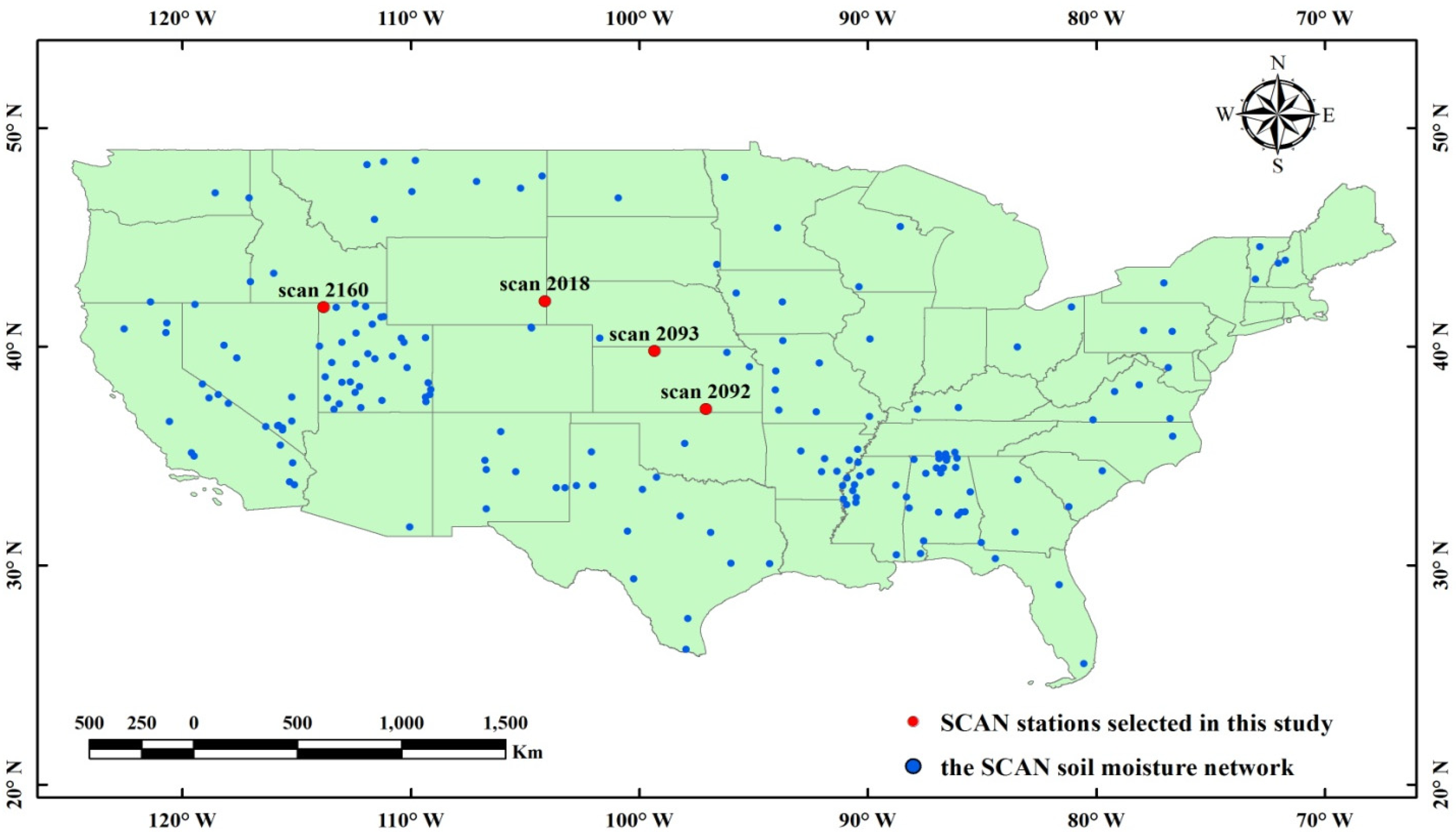
In this paper, we focused on the estimation of the soil roughness parameter Hr. Considering the coarse spatial resolution of the AMSR-E observations, over a given pixel, the time changes in the effects of surface roughness are mixed over a variety of land cover types. Therefore, compared to the time variability, we assumed in this study that the spatial variability of the Hr parameter is more critical. Based on AMSR-E 6.9 GHz TB (brightness temperature) observations, SMOS soil moisture products and ECMWF’s soil temperature, we developed a simple approach to globally estimate the spatial variations in the parameter Hr. The method was first applied over a few sites from the SCAN network in the USA to illustrate the proposed method. In the second step, global maps of the Hr parameter were produced.
3. Method
This study was based on the τ − ω [
22] model with the assumption of a low influence from atmospheric effects and neglecting the multiple scattering effects in the vegetation. The brightness temperature
TBp can be expressed as a three-component model (Equation (2)). The first part is the upward radiation from vegetation, the second part is the downward vegetation emission reflected by the soil and then attenuated by the canopy, and the last part is the soil emission attenuated by the vegetation canopy.
where
TG and
TC are the effective soil and vegetation temperature,
rG is the soil reflectivity,
γ is the vegetation attenuation factor and
ω is the single scattering albedo of the canopy;
θ is the incidence angle of the observations. The parameter
ω accounts for the effects of canopy volume scattering [
22]. However, there is limited information on the temporal or canopy type variability of this parameter, and most of the
SM retrieval algorithms considered the use of a constant global value [
51]. Van de Griend and Owe [
52] showed that
ω had a low effects on the range of the emitted radiation from vegetated surfaces at microwave wavelengths [
7,
51]. For simplicity, as in several other studies at C-band, it is assumed in this study that
ω, considered here as an effective parameter [
53], is equal to zero [
1,
7,
52]. Furthermore,
TC and
TG are assumed to be equal at 6 am and represented as
T [
54]. These assumptions lead to the following simplified equation [
55]:
The soil reflectivity
rG can be written as a function of the reflectivity of a flat surface
, a set of four soil roughness parameters (
Hr,
Q,
Nrp,
p =
V or
p =
H), incidence angle
θ and polarization
p, as [
19]:
where
Q is the polarization mixing parameter [
7],
Hr is a parameter related to the intensity of the roughness effects and
Nrp expresses the angular dependency of the roughness effects [
56]. An increase in the value of the
Q parameter generally leads to a decrease in the difference between
TBH and
TBV (
TBH increases and
TBV decreases). Wang
et al. [
57] have found that the frequency dependence of
Q is strong and relatively small values for
Q were obtained, ranging from 0 to 0.12 at L-band and from 0 to 0.3 at C-band. More recently, Montpetit
et al. [
27] have found that the value
Q = 0.075 can be used over a large frequency range (1.4–90 GHz). In this study, we considered the value of
Q is equal to zero, but a sensitivity analysis is made for
Q varying from 0 to 0.3. Following the result obtained by [
23], the values of
Nrp for the
H and
V polarizations were set equal, and we assumed that
NrH =
NrV = 0 [
23]. According to the Fresnel equations,
at a specific incidence angle is only related to the soil dielectric properties (
εp). In the present study,
εp was estimated using the Mironov model [
57]. The inputs of the Mironov model in this study were (i)
SM estimated from the SMOS observations, (ii) the soil effective temperature provided by the ECMWF products and (iii) the clay fraction (%) estimated from the FAO maps.
The vegetation attenuation factor (
γ) was expressed as the function of the optical depth
τp as:
and the vegetation optical depth
τp can be calculated from the optical depth at nadir (at
θ = 0) as [
26]:
where
ttp is a specific vegetation parameter accounting for the effects of the vegetation structure. The
ttp parameters allow accounting for the dependence of
τnad on incidence angle. A value of
ttp > 1 or
ttp < 1 will correspond, respectively, to an increasing or decreasing trend of
τnad as a function of
θ, and the case
ttH =
ttV = 1 corresponds to isotropic conditions, when the optical depth of the standing canopy is assumed to be independent of both polarizations and incidence angles. Some experimental evidence has shown that there is a difference in vegetation attenuation properties between the
H and
V polarizations over agricultural fields, mainly for vertical stem-dominated vegetation (such as wheat or corn) [
14]. However, the canopy and stem structure for most crops and naturally occurring vegetation are randomly oriented. Moreover, considering that at coarse spatial resolution the pixel includes a variety of vegetation types, so that the specific effects related to the structure of a variety of vegetation canopies are mixed together, it is reasonable to assume that the optical depth is polarization-independent (
ttH =
ttV = 1) [
51,
52,
58].
Previous studies, such as Schmugge
et al. [
59] and Jackson
et al. [
6] combined the vegetation optical depth and roughness effects within a single parameter (referred to as the α parameter) to retrieve soil moisture. Similarly, Njoku & Chan [
7] and Saleh
et al. [
60] used this α parameter to approximate the combined effects of vegetation and roughness. Consequently, in this study, substituting Equations (5) and (6) in Equation (3), we can obtain:
with
Considering the
H and
V polarizations, the a parameter can be derived as [
61]:
In the following of this study we considered the parameter
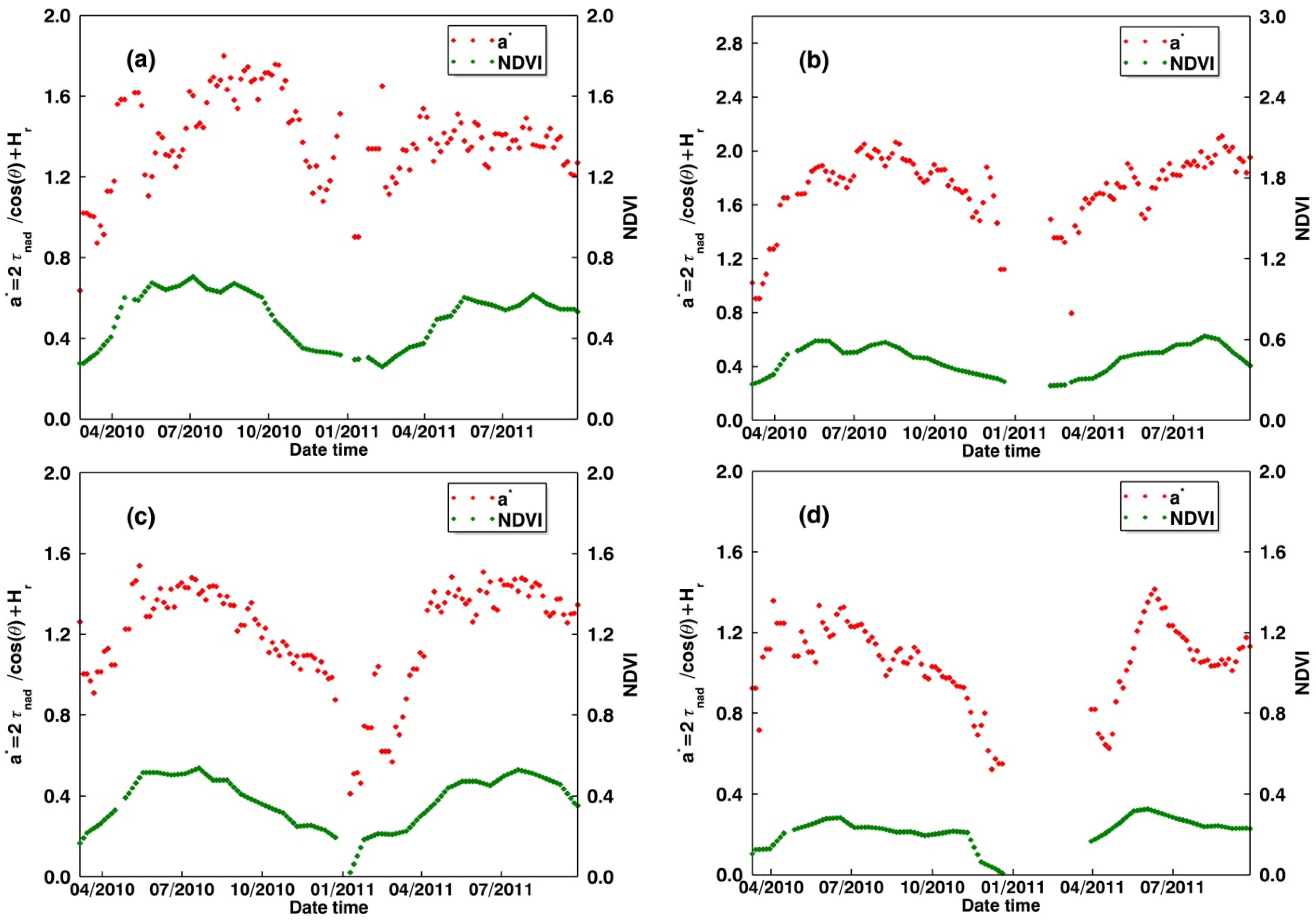
a* defined as follows:
From this equation,
a*(
θ) can be seen as a parameter accounting for the combined effects of vegetation (through the
τnad parameter) and surface roughness (through the
Hr parameter) [
26]. The parameter
a*(
θ) at a given incidence angle can be directly calculated from the horizontal and vertical polarization brightness temperatures using Equation (9). In this study, the
a*(
θ) parameter was calculated with only one angle and for ease of reading it is noted
a* in the following of the text.
We used the NDVI index in an attempt to decouple the vegetation and surface roughness effects in Equation (10). To this aim, we assumed that optical depth can be linearly related to the vegetation index NDVI [
39,
62,
63]. Note that errors may arise from this assumption, as a linear relationship between optical depth and NDVI is only suitable for vegetation canopies with a rather low biomass [
63]. In particular, NDVI is likely to saturate more rapidly than optical depth (due primarily to the deeper penetration capabilities of the microwave radiations) over dense canopies in forested regions. We assumed too that the attenuation effects of vegetation are very low for low values of NDVI, so that roughness effects are dominant (
a* ≈
Hr) when
VI ≈ 0.
Using these assumptions, at a given incidence angle, the parameter
a* can be expressed as a function of NDVI over each pixel as:
where
A is a slope parameter which has to be calibrated over each pixel.
Equation (11) was used to compute the value of Hr over each pixel. For this purpose, a standard statistical procedure was applied to compute the slope and intercept of regression Equation (11) using values of the NDVI index estimated from MODIS and values of a* computed from the AMSR-E observations (using Equation (9)).
In this process, we considered two main cases:
“Bare or sparsely vegetated surfaces”, corresponding here to the case when the effects of the vegetation layer, could be considered negligible over a sufficient period of time (this case was arbitrarily defined here as when 15% of the NDVI values were lower than 0.07 in the whole NDVI time series [
64]).
In that case, we set the surface roughness Hr as the average value of a* under the condition of NDVI values lower than 0.07. This case included the case of deserts, where the NDVI values where always lower than 0.07. In that latter case, we set the value of Hr as the average value of a*.
- 2.
“Vegetated surfaces” corresponding here to the case when the effects of the vegetation layer are significant over most of the dates of the considered dataset (case defined as: more than 85% of the NDVI values exceed the threshold value of 0.07).
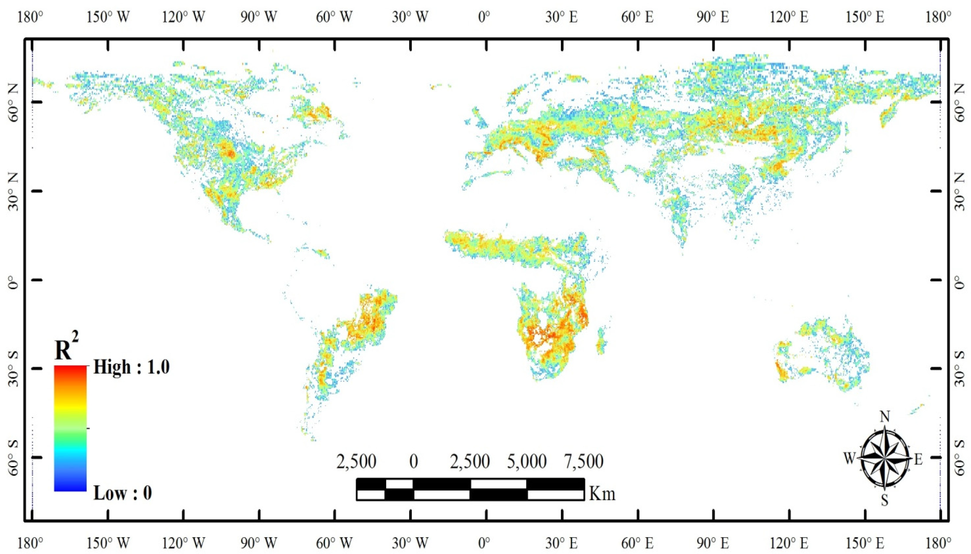
In that case, we set the surface roughness Hr as the intercept of the regression Equation (11), linking a* to NDVI. Note that the values of Hr were computed only over nodes where (i) the correlation was significant (p-value < 0.05) and where (ii) the coefficient of determination R2 was higher than a threshold value set arbitrarily here to 0.2 (R2 > 0.2). This filtering was conducted in order to compute values of Hr from the value of the intercept of the regression line only when there was a well-defined correlation between a* and NDVI.
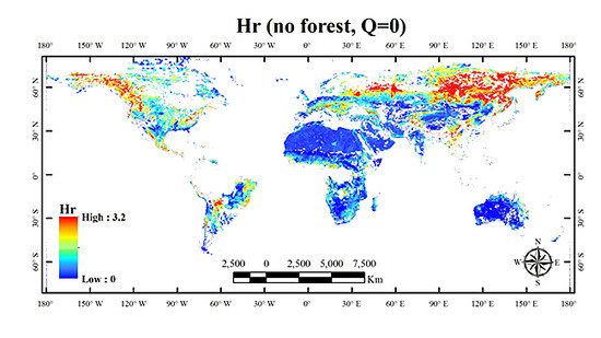
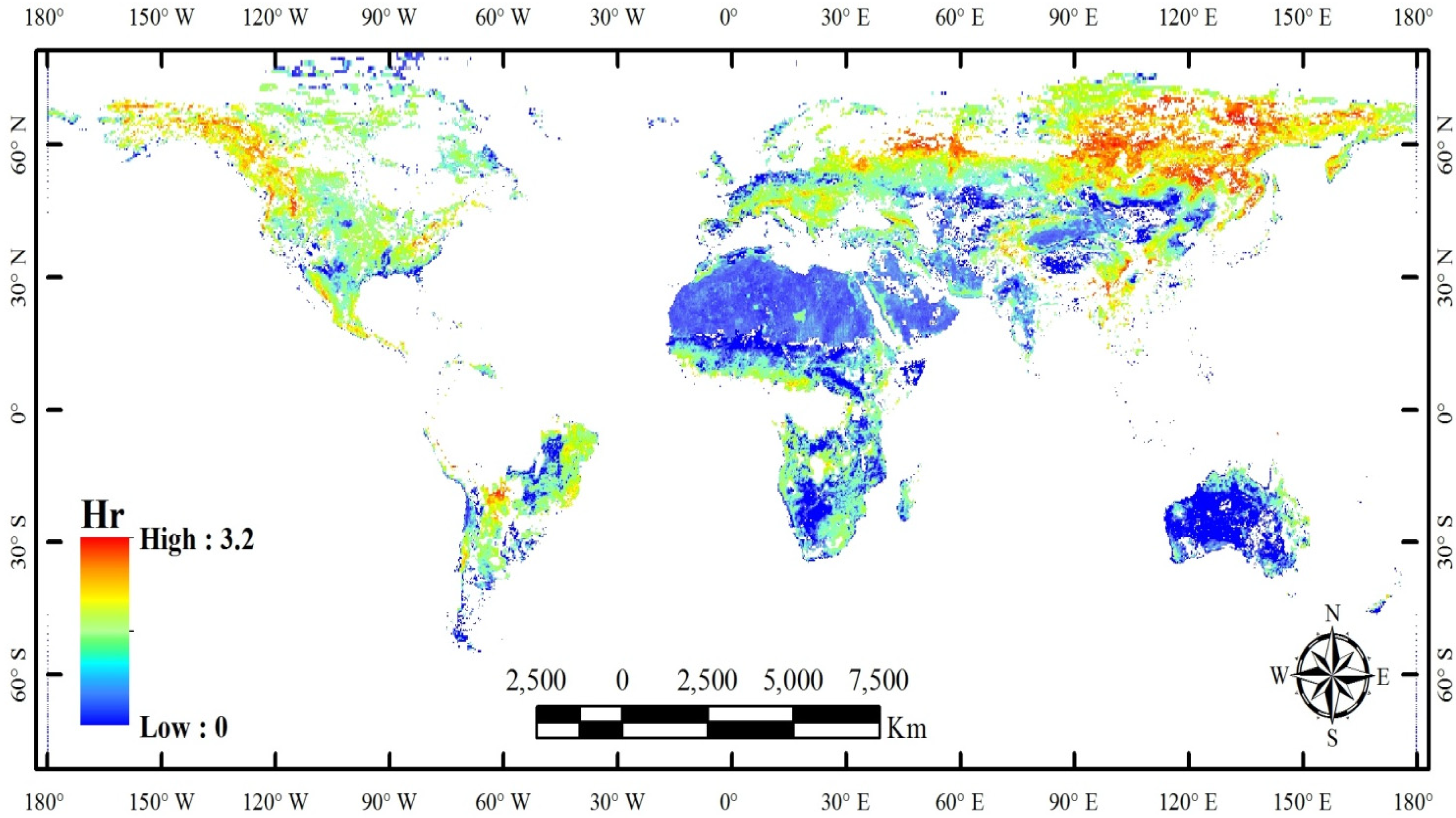
Following that procedure over all pixels, we could compute a global map of the parameter Hr, except over regions of dense forests, which were masked out.
5. Conclusions
A first attempt to compute global maps of the Hr parameter was carried out in this study, based on AMSR-E observations. With the methods described, we attempted to correct for the vegetation effects, and regions classified as broadleaf evergreen forests were masked out. However, it is likely that a larger uncertainty is associated with the retrieved values of
Hr for pixels covered by relatively dense vegetation covers and in forested areas. For instance, high
Hr values were retrieved in many forested regions, such as in northern Asia and northwestern regions of America, which were mainly covered by evergreen and deciduous coniferous forests, and central and southern regions of China, which were mainly covered by deciduous broadleaf forests. This may be caused by the saturation of the NDVI values over forests, where the linear relationship between NDVI and vegetation optical depth may be not valid. Even though vegetation effects could not be perfectly corrected in densely vegetated regions, it is likely the global map of
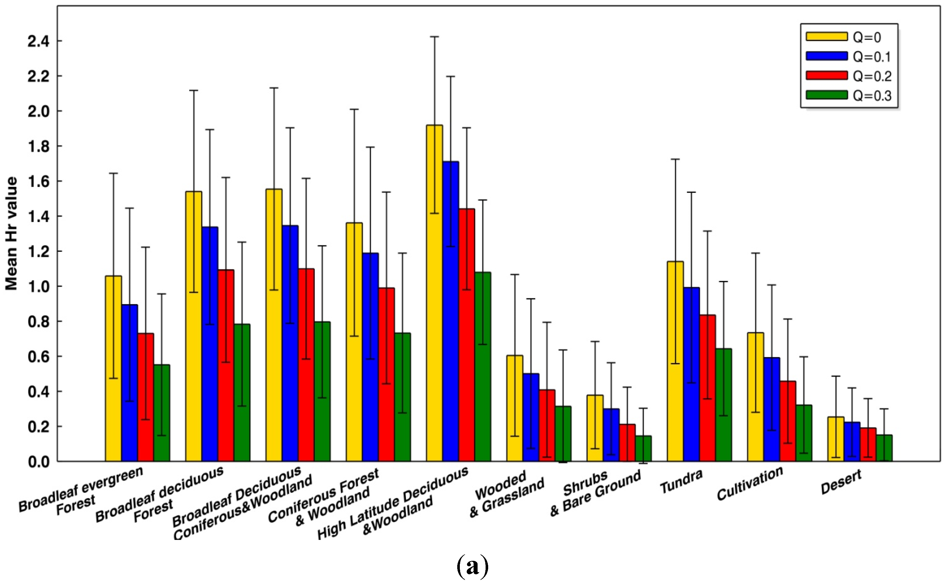
Hr computed in this study could represent the main spatial patterns of the surface roughness effects in low vegetated regions. We found that clear spatial patterns could be distinguished in the global maps and could be associated with the main cover types (
Table 2). It is important to note that the
Hr parameter is a complex synthetic parameter which accounts for many effects, such as surface roughness, soil moisture heterogeneities [
18,
67], vegetation litter in prairies and forests [
41,
60,
67,
68], topography [
69],
etc. These different effects occur over a large domain of spatial scales. This means the interpretation of the obtained global maps of
Hr remains difficult. Nevertheless, it seems that higher values of
Hr were generally obtained in forested areas. It likely that this result is related to the effects of vegetation, which may not be totally corrected. However, this result may be related also to the effects of litter which are generally taken into account through the
Hr parameter. For instance Grant
et al. [
68] have retrieved values of
Hr greater than 0.1 to account for the effects of litter over both a coniferous and a deciduous forest in flat experimental sites. Larger values of
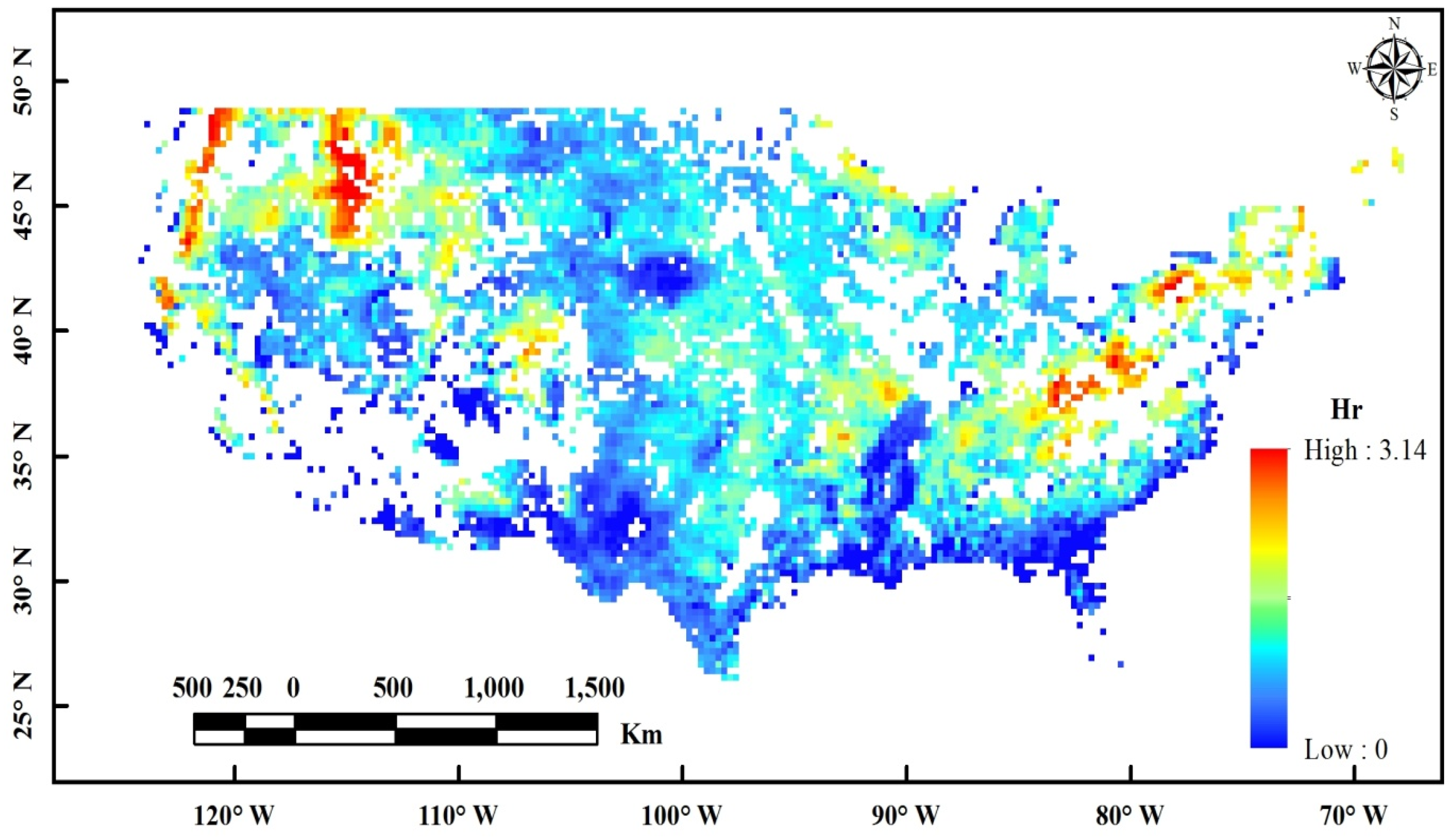
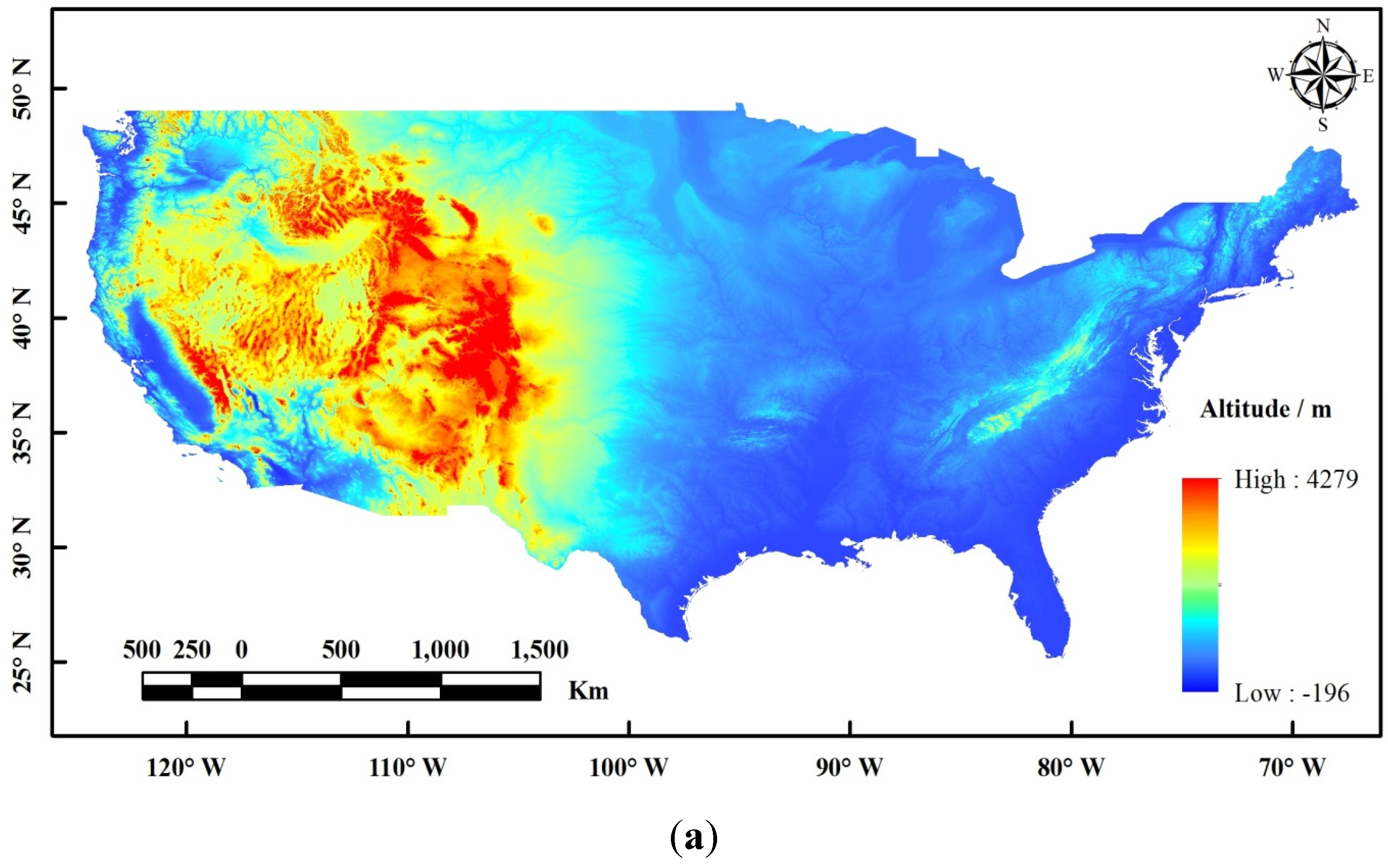
Hr were also obtained in hilly regions, as found in the results illustrated for the USA in
Section 4. It seems this result confirms the fact that
Hr is an effective parameter which may be used to account for the effects of topography in SM retrieval studies at coarse spatial resolution.
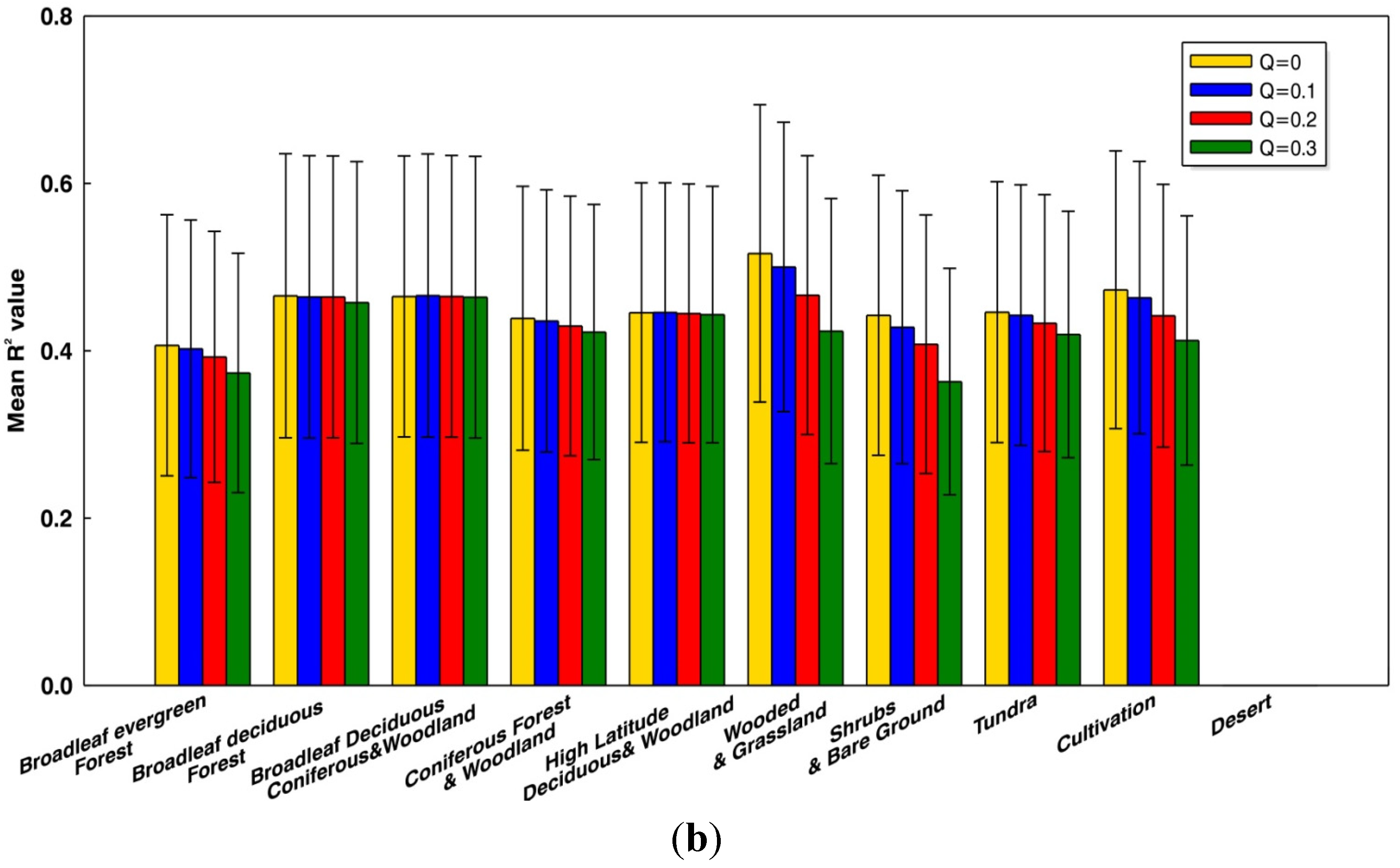
All the results presented in this study are sensitive to the assumptions made in our modeling approach. In particular, we found that the global maps of
Hr we obtained were sensitive to the value selected for the
Q parameter. Retrieved Hr values would significantly decrease if we used a higher
Q value such as
Q = 0.3. Hence, the maps presented in this study are valid for low values of the
Q parameter, which is an assumption often made at C-band [
18]. Moreover, a recent study [
27] has confirmed the fact that a low value of the
Q parameter can be used to model the effects of roughness over a large frequency range. Note also that the use of large values of
Q make the decoupling between the roughness and vegetation effects more difficult (lower values were obtained in the
R2 values of the relationship between
a* and NDVI over all types of biomes).
In future studies, we will evaluate whether the global maps of Hr computed in this study have the potential for improving soil moisture retrieval for present and future spaceborne microwave remote sensing missions at the C-band.


 ,
, 


