1. Introduction
The characterization of plant nutrients, e.g., nitrogen (N) and phosphorus (P), is important to understand the process of plant growth in natural ecosystems [
1] and helps to understand the foraging behavior, habitat selection and migration of some animals [
2,
3]. Over the last four decades, the advances in reflectance spectroscopy, airborne and satellite technology have made it feasible to be more independent of routine wet-chemistry analyses for plant nutrients, and they have provided opportunities for scientists to understand the temporal and spatial changes of plant nutrients at a landscape or regional scale [
4,
5,
6,
7,
8,
9]. Among these studies, univariate regression with vegetation indices (VIs) and multivariate regression methods are commonly used to extract useful information for nutrient characterization. These modeling methods provide convenient and interpretable means for researchers to understand the fundamental interaction of plant condition with radiant energy detected by multispectral or hyperspectral sensors [
4,
5,
6,
7,
9,
10,
11,
12,
13,
14,
15,
16].
Since Pearson and Miller [
17] proposed the first two VIs,
i.e., the ratio vegetation index (RVI) and vegetation index number (VIN) for estimating grass productivity, many followers have proposed and improved hundreds of VIs to minimize solar irradiance and soil background effects and to enhance the vegetation response further [
6,
11,
15,
18,
19,
20,
21,
22,
23,
24,
25]. Generally, the VIs are classified into two large categories: (i) broadband VIs, which are derived from the reflectance of multispectral sensors (e.g., Landsat MSS, Landsat TM, SPOT, AVHRR and MODIS); and (ii) narrowband VIs, which are derived from the reflectance of hyperspectral sensors, including ground-based (e.g., ASD FieldSpec portable spectroradiometer), airborne (e.g., Hymap) and spaceborne (e.g., Hyperion) sensors. Some studies demonstrated that narrowband VIs could overcome the saturation problem commonly occurring for broadband VIs for biomass estimation in dense vegetation [
20]. Recent studies further demonstrated the successful applications and high prediction accuracies of narrowband VIs in estimating plant nutrients (e.g., N) [
6,
12,
13,
15,
21,
23,
24,
25]. Apart from the traditional simple ratio index (SRI) and normalized difference index (NDI), which contain only two spectral bands, the three-band index (TBI) and red edge parameters (e.g., red edge position (REP)) have also been reported to result in higher prediction accuracy for nutrient estimations. For example, Tian
et al. [
24] and Pacheco-Labrador
et al. [
15] respectively compared the performances of 61 and 82 published VIs for N estimations, and they claimed their newly proposed TBIs improved prediction accuracy. However, their studies showed that these aforementioned VIs are sensitive to specific vegetation species, growth stages and study areas.
Since the early attempt at estimating the N content in sweet pepper leaves from laboratory-based reflectance with univariate regression [
26], many researchers have used linear or non-linear multivariate regressions for plant nutrient estimations, such as stepwise multiple linear regression (SMLR) [
5,
6,
8,
27], partial least squares regression (PLSR) [
5,
9,
27] and support vector regression (SVR) [
14,
28]. SMLR is the linear combination of several important bands selected from the whole reflectance spectra; however, it has the potential problem of over-fitting [
29]. PLSR can overcome the problem of multicollinearity commonly existing between narrow hyperspectral bands, because it compresses the whole spectra into several latent variables. SVR has the advantage of extracting non-linear relationships from reflectance spectra. Although some studies reported that PLSR and SVR could improve the prediction accuracy compared with SMLR [
5,
27,
30], such results were obtained at the expense of increasing model complexity due to the use of whole spectra for modeling. Moreover, in order to acquire higher prediction accuracy when employing the multivariate regression methods, the original reflectance spectra often require some pre-processing methods, such as first derivative analysis [
9,
31], absorbance [
5], continuum-removal [
6,
8] or water-removal analysis [
27]. However, the different choice of spectral pre-processing methods may yield completely different prediction results. Therefore, the choice of pre-processing and multivariate regression methods makes it difficult to balance between model accuracy and simplicity.
The successive projections algorithm combined with multiple linear regression (SPA-MLR) proved to be a time-saving and robust method for multivariate calibration [
32], and it has been successfully applied to many fields of research, such as spectroscopic chemical analysis [
33,
34] and grass nutrient assessment [
31]. SPA selects informative wavelengths by using simple operations in a vector space to minimize variable collinearity [
32]. Cui
et al. [
31] reported that SPA-MLR outperformed PLSR with higher prediction accuracy and better model simplicity and confirmed the advantage of SPA-MLR in grass nutrient estimation using laboratory-based reflectance.
However, it is still unknown whether SPA-MLR is comparable to PLSR in grass nutrient estimation with canopy reflectance data, because canopy spectra are popularly used in vegetation studies, and they can better characterize the actual status of vegetation than leaf spectra. Little guidance and few comprehensive comparative studies have been offered to choose among the aforementioned methods (i.e., univariate regression with VIs, multivariate regression methods and SPA-MLR) for estimating grass nutrients at the canopy level. Moreover, it also remains unknown whether the optimal method is consistent in estimating different nutrient elements.
The performance of a statistical model using hyperspectral reflectance is often evaluated by predictive accuracy,
i.e., determination coefficient (R
2), root mean square error (RMSE) and ratio of prediction to deviation (RPD) [
14,
20,
27,
31,
35,
36]. However, little information of model simplicity, robustness and interpretation can be gained from the predictive accuracy. A simple model should confirm the notion of Occam’s razor [
37]; a robust model should be unbiased and transferable (both temporally and spatially) [
29,
38]; and an interpretable model should consider physical meaning for the included spectral bands [
10,
15,
18]. Therefore, it is recommended to synthetically consider predictive accuracy, simplicity, robustness and interpretation for evaluating model performance.
Carex cinerascens is a wetland grass species widely distributed in Poyang Lake, China, and it is the main food for some over-wintering birds, such as the swan goose (
Anser cygnoides) and white-fronted goose (
A. albifrons albifrons) [
39]. This study aimed to evaluate the performances of univariate linear regression with nine published VIs, three classical multivariate regression methods (SMLR, PLSR and SVR) and SPA-MLR in estimating the nutrients (N and P) of
C. cinerascens with canopy hyperspectral reflectance. Such comparison might help to understand their comprehensive performance from the perspective of model accuracy, simplicity, robustness and interpretation and would provide guidance in selecting the optimal method for estimating plant nutrients at various levels.
2. Material and Methods
2.1. Sampling Design and Canopy Spectral Measurements
The study was carried out in Poyang Lake (28°52′21″−29°06′46″N, 116°10′24″−116°23′50″E), Jiangxi Province, China. As the largest freshwater lake in China, Poyang Lake is an important wetland in the world for bird over-wintering. In order to obtain a large variation of N and P contents for modeling, field sampling was designed in different growth stages of C. cinerascens. Two field surveys were carried out from 4−7 December 2012 (vegetative stage) and from 10−15 April 2013 (heading stage), respectively, when Poyang Lake was in dry seasons. In each field survey, nine sites (150 × 150 m), which could be physically measured without interference caused by deep water, were randomly arranged within large areas of C. cinerascens. At each site, four to eight plots (1 × 1 m) were randomly laid out to keep at least 30 m apart between any two plots. Due to dense canopy cover (nearly 100%), very little soil beneath C. cinerascens in each plot could be seen from above the canopy. The canopy spectra and leaf samples for 66 and 71 plots were measured and collected in 2012 and 2013, respectively, following the same procedure: (i) the longitude and latitude coordinates at each plot were obtained using a global position system receiver (Garmin Ltd., Lenexa, KS, USA); (ii) prior to each spectral measurement, a calibrated white Spectralon panel was used to minimize the effect of changes of solar irradiance and atmospheric conditions on canopy reflectance; (iii) ten successive spectra (350–2500 nm, 2151 spectral bands) were measured 1 m above the canopy at nadir position using an ASD FieldSpec® 3 (spectral resolution: 3 nm at 700 nm and 10 nm at 1400/2100 nm; sampling interval: 1.4 nm at 350–1050 nm and 2 nm at 1000–2500 nm) portable spectroradiometer (Analytical Spectral Devices, Inc., Boulder, CO, USA) with a field of view of 10°; (iv) after spectral measurement, the subplots of 0.25 × 0.25 m in the four corners and center of each plot were harvested by clipping leaves (5 cm above the ground) and merged; and (v) the merged fresh leaves were immediately put into a labeled sample bag for their chemical analyses.
2.2. Chemical Analysis
The collected leaf samples were dried at 70 °C for 24 h in an oven, ground with an agate mortar and passed through a 65-mesh sieve (0.25 mm). The dried and ground samples were initially pre-processed by HCLO
4−H
2SO
4 digestion. Following digestion, N content (%) was measured with the semi-micro Kjeldahl method [
40], and P content (%) was determined using the MO-Sb (molybdenum-antimony) colorimetric method [
41]. To ensure measurement accuracy, certified house reference materials and reagent blanks were used during chemical analyses.
2.3. Spectral Pre-Processing
For each sampling plot, the collected ten successive spectra were averaged as the final spectrum. Due to the large noises at edges and the water absorption regions of each spectrum, the raw canopy spectra were reduced from 2151 wavebands (350–2500 nm) to 1603 wavebands, including three spectral portions (
i.e., 400−1350, 1450−1750 and 2050−2400 nm). Because some vegetation indices (VIs), such as red edge position (REP), use 1st derivative spectra, the spectra were then subjected to first derivative analysis using the Savitzky–Golay filter to reduce the effects of multiple scattering of radiation [
12,
42]. The spectral pre-processing and subsequent modeling were implemented with PLS_Toolbox 7.3 (
http://www.eigenvector.com/software/pls_toolbox.htm) based on MATLAB 7.11 (The MathWorks, Inc., Natick, MA, USA).
2.4. Modeling Methods
2.4.1. Univariate Linear Regression with VIs
In this study, we employed nine narrowband VIs (
Table 1) that were recently proposed for N or N-related component estimations to establish univariate linear relationships with N and P contents. These VIs were derived from canopy hyperspectral reflectance measured by spectroradiometers. Apart from TBI3 applied in forest ecosystem, the other eight VIs were applied in farmland ecosystem. The VIs can mainly be classified into four groups: simple ratio index (SRI), normalized difference index (NDI), three-band index (TBI) and red edge parameters, e.g., red edge position (REP). To date, very few studies have used VIs for P estimation [
43,
44]. Therefore, univariate linear regression models with these VIs (the name of the VI was noted as the univariate linear regression model with the VI for simplicity) were built for the N and P estimations of grass species (e.g.,
C. cinerascens).
Table 1.
Nine published vegetation indices (VIs) for N or N-related component estimation using canopy hyperspectral reflectance. SRI, simple ratio index; NDI, normalized difference index; TBI, three-band index.
Table 1.
Nine published vegetation indices (VIs) for N or N-related component estimation using canopy hyperspectral reflectance. SRI, simple ratio index; NDI, normalized difference index; TBI, three-band index.
| VIs | Formula | Plant Species | R2Val | Literature |
|---|
| SRI1 | | Wheat | 0.847 | Yao et al. [23] |
| SRI2 | | Sugarcane | 0.760 | Abdel-Rahman et al. [12] |
| SRI3 | | Corn | 0.706 | Corp et al. [22] |
| NDI1 | | Wheat | 0.836 | Yao et al. [23] |
| NDI2 | | Corn | 0.672 | Corp et al. [22] |
| TBI1 | | Rice | 0.830 | Tian et al. [24] |
| TBI2 | | Rice | 0.866 | Wang et al. [25] |
| Wheat | 0.883 |
| TBI3 | | Holm oak | 0.760 | Pacheco-Labrador et al. [15] |
| REP | | Maize Rye | 0.860 | Cho and Skidmore [21] |
| 0.820 |
2.4.2. Classical Multivariate Regression Methods
Three multivariate regression methods (SMLR, PLSR and SVR) have been popularly employed for N and P estimations of plants at leaf, canopy and landscape levels (
Table 2). These methods often employ pre-processed spectra (e.g., continuum-removed, absorbance, 1st derivative and water-removed spectra) for modeling to improve predictive accuracy.
Table 2.
A list of some literature on N and P estimations using multivariate regression methods. SMLR, stepwise multiple linear regression; PLSR, partial least squares regression; SVR, support vector regression.
Table 2.
A list of some literature on N and P estimations using multivariate regression methods. SMLR, stepwise multiple linear regression; PLSR, partial least squares regression; SVR, support vector regression.
| Method | Reflectance Spectra Used | N (R2Val | RMSEVal) | P (R2Val | RMSEVal) | Literature |
|---|
| SMLR | Canopy, continuum-removed | 0.700–0.760 | 0.310–0.460 | Mutanga et al. [6] |
| SMLR | Leaf, absorbance | | 0.232 | 0.087% | Bogrekci and Lee [5] |
| SMLR | Image, continuum-removed | 0.210 | | Ullah et al. [8] |
| SMLR | Canopy, 1st derivative | 0.590 | 0.450% | 0.250 | 0.080% | Ramoelo et al. [27] |
| SMLR | Canopy, water-removed | 0.870 | 0.250% | 0.640 | 0.060% | Ramoelo et al. [27] |
| PLSR | Canopy, 1st derivative | 0.590 | 0.450% | 0.470 | 0.070% | Ramoelo et al. [27] |
| PLSR | Canopy, water-removed | 0.840 | 0.280% | 0.430 | 0.070% | Ramoelo et al. [27] |
| PLSR | Leaf, absorbance | | 0.425 | 0.073% | Bogrekci and Lee [5] |
| PLSR | Canopy, 1st derivative | 0.830 | 0.210% | 0.770 | 0.050% | Sanches et al. [9] |
| SVR | Image, original | 0.030–0.673 | | Karimi et al. [28] |
| SVR | Leaf, 1st derivative | 0.706 | 0.521% | 0.722 | 0.073% | Zhai et al. [14] |
| SVR | Leaf, original | 0.197 | 0.946% | 0.458 | 0.097% | Zhai et al. [14] |
SMLR starts with no selected variable (wavelength) and searches the best single wavelength at each iteration based on the highest F-statistic value or the lowest
p-value [
12]. SMLR computes the F-statistic and
p-values for each wavelength, and it removes irrelevant wavelengths based on predefined removal F-statistic or
p-values. The procedure stops at the
n-th iteration when
n wavelengths are selected. The entry and removal of
p-values were set at 0.05 and 0.10 based on empirical settings, respectively. To minimize the over-fitting problem of SMLR, the
M/
N ratio (
M = the number of selected wavelengths,
N = the number of calibration samples) suggested by Thenkabail
et al. [
11] and variation inflation factor (VIF) described by Neter
et al. [
45] were employed. The
M/
N ratio and VIF did not exceed 0.15–0.20 and 5–10, respectively. The optimum number of selected wavelengths was determined by the best SMLR model with the highest prediction accuracy based on the test set.
PLSR brings together the advantages of principal component analysis (PCA), canonical correlation analysis (CCA) and MLR [
46]. Unlike PCA, PLSR compresses predictor variables into several latent variables (LVs) to capture both of the greatest variance of predictor variables and the maximum correlation between the LV scores and dependent variables (e.g., N or P contents) [
7,
29,
46]. The details of PLSR can be found in Geladi and Kowalski [
46]. The optimum number of LVs was determined by leave-one-out cross-validation procedure. To prevent collinearity and over-fitting, the root mean square error of cross-validation (RMSE
CV) should be reduced by >2% when adding an extra LV to the PLSR model [
7,
47].
Unlike SMLR and PLSR, SVR is a non-linear statistical learning technique. SVR computes a linear regression function in a high dimensional feature space, in which the input data are mapped by a non-linear function [
48]. Moreover, it optimizes the generation error in order to obtain the best generalized performance on a limited number of support vectors (SVs) [
48,
49]. The details of SVR can be found in Smola and Schölkopf [
48]. The optimization process was tuned by a systematic grid search of the parameters using five-fold cross-validation [
29].
2.4.3. SPA-MLR
The successive projections algorithm (SPA) proposed by Araújo
et al. [
32] is a forward selection method in order to minimize variable collinearity. In a nutshell, SPA starts with one wavelength and selects a new one at each iteration by using projection operators in a vector space until reaching the predefined number of wavelengths. The new selected wavelength has the maximum projection value on the orthogonal subspace of the previous selected wavelengths [
50]. Unlike genetic algorithm (GA), which is a popular variable selection method based on survival of fittest theory, SPA is a deterministic search technique, and it is more robust according to the choice of validation samples [
32]. MLR was employed to establish the relationship between the wavelengths selected by SPA and dependent variables (N or P contents). To prevent over-fitting and to obtain the best SPA-MLR model, the maximum and optimum number of selected wavelengths were determined following the same method used for SMLR (see
Section 2.4.2). SPA was implemented using SPA_GUI 1.0 (
www.ele.ita.br/~kawakami/spa) based on MATLAB 7.11 (The MathWorks, Inc., Natick, MA, USA).
2.5. Model Development
For N or P estimation using the 13 aforementioned modeling methods, preliminary experiments showed that the predictive accuracies were very poor (R
2 < 0.30) with the two original datasets (
Table 3) for the training set and test set; this might because the nutrient contents in the original datasets had a narrow range and imbalanced statistical distribution [
7]. Thus, the original datasets collected over two growth stages were combined into a single dataset, and its N and P contents were sorted from the lowest to highest values, respectively. The combined dataset was then partitioned into two datasets following the partitioning strategy given by Kemper and Sommer [
35]. The odd-numbered samples were selected as the training (or calibration) set, while the even-numbered samples as the test (or validation) set (
Table 3). The new training set and test set had similar statistical distribution of nutrient contents, and they provided a much wider range and higher coefficient of variation of nutrient contents than the original datasets. To some extent, this data partitioning could avoid the unbiased estimation. For each modeling method (see
Section 2.4) in N and P estimations, the training set was used for model calibration and cross-validation, and the test set was applied for model validation.
In this study, three VIs (SRI2, SRI3 and REP), three multivariate regression methods (SMLR, PLSR and SVR) and the SPA-MLR method employed the 1st derivative spectra for modeling, while the other six VIs (i.e., SRI1, NDI1, NDI2, TBI1, TBI2 and TBI3) used the original spectra following the original formula. Therefore, a total of 13 models were established for N and P estimations, respectively.
Following the suggestion of Wise
et al. [
29], prior to modeling, the dependent variables (N or P contents) and independent variables (VIs or 1st derivative spectra) were processed with the autoscaling method to obtain a uniform dimension. This method uses mean-centering followed by dividing each variable by the standard deviation of the variables [
29]. The determination coefficient of cross-validation and validation (R
2CV and R
2Val), the root mean square error of cross-validation and validation (RMSE
CV and RMSE
Val), the ratio of prediction to deviation (RPD, the ratio of the standard deviation of the reference values in the test set to RMSE
Val) and the bias for validation were calculated for each model. Further, due to using the whole spectra for modeling, PLSR and SVR had much more complicated model equations than the VIs, SMLR and SPA-MLR, which employed a limited number of predictor variables. Thus, only the optimum number of LVs and SVs was reported for PLSR and SVR models, respectively.
Table 3.
Descriptive statistics of N and P contents.
Table 3.
Descriptive statistics of N and P contents.
| | Nutrient | Dataset | n | Range (%) | Mean (%) | CV (%) |
|---|
| Original data | N | December 2012 | 66 | 1.73−3.08 | 2.44 | 14.56 |
| April 2013 | 71 | 1.00−2.07 | 1.59 | 12.98 |
| P | December 2012 | 66 | 0.17−0.41 | 0.28 | 17.51 |
| April 2013 | 71 | 0.08−0.20 | 0.16 | 13.57 |
| Data partitioning | N | Training set | 69 | 1.00−3.08 | 2.00 | 26.03 |
| Test set | 68 | 1.12−3.06 | 2.00 | 25.38 |
| P | Training set | 69 | 0.08−0.41 | 0.22 | 33.06 |
| Test set | 68 | 0.18−0.37 | 0.22 | 31.68 |
2.6. Model Comparison
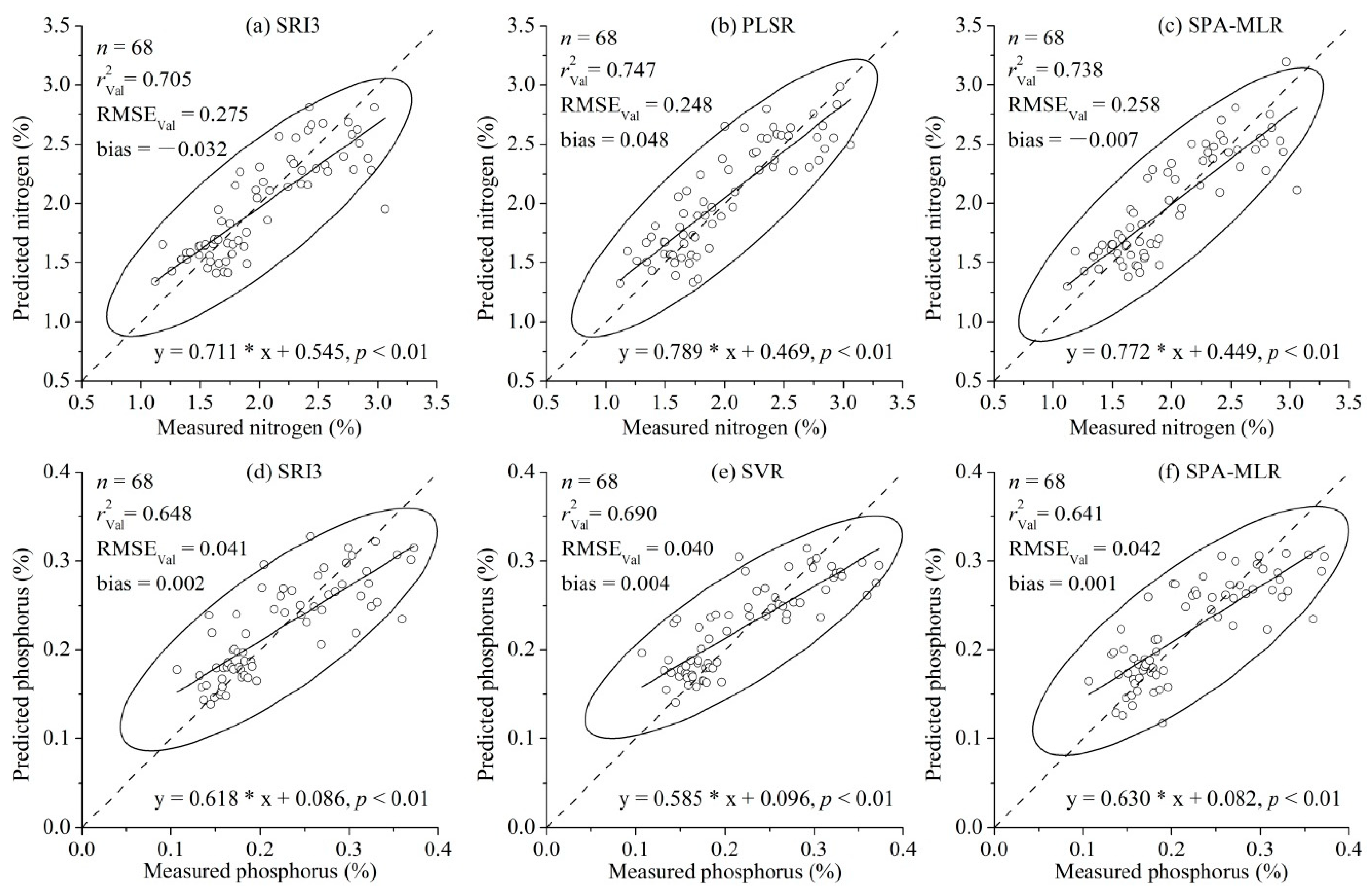
The 13 statistical models for N estimation were compared based on their prediction performances (R2Val, RMSEVal, RPD and bias), respectively. Afterwards, the best-performing VI and classical multivariate regression models with the highest predictive accuracy were chosen to be compared with the SPA-MLR model for N estimation, according to the slope and intercept values for the fitting line between predicted and measured values. The aforementioned methods were employed for comparison of the 13 statistical models for P estimation. Moreover, in order to synthetically explore the significant differences between SPA-MLR and the other modeling methods for nutrient (N and P) estimation, one-way analysis of variance (ANOVA) using the least squares difference (LSD) method was performed considering the mean R2Val values of the 13 methods for N and P estimations.


