Article

Analysis of the Land Surface Temperature Scaling Problem: A Case Study of Airborne and Satellite Data over the Heihe Basin

1
State Key Laboratory of Remote Sensing Science, Institute of Remote Sensing and Digital Earth, Chinese Academy of Sciences, Beijing 100101, China
2
Joint Center for Global Change Studies (JCGCS), Beijing 100875, China
3
College of Resources and Environment, University of Chinese Academy of Sciences, Beijing 100049, China
*
Authors to whom correspondence should be addressed.
Remote Sens. 2015, 7(5), 6489-6509; https://doi.org/10.3390/rs70506489
Submission received: 12 December 2014 / Accepted: 19 May 2015 / Published: 22 May 2015

Abstract

:
This study analyzed the scaling problem of land surface temperature (LST) data retrieved with the Temperature Emissivity Separation (TES) algorithm. We compiled a remotely sensed dataset that included Thermal Airborne Hyperspectral Imager (TASI) and satellite-based Advanced Spaceborne Thermal Emission Reflection (ASTER) data, which were acquired simultaneously. This dataset provided the range of spatial heterogeneities of land surface necessary for the study, which was quantified by the dispersion variance. The LST scaling problem was studied by comparing the remotely sensed LST products in two ways. First, the LST products calculated in the distributed method and the lumped method were compared. Second, the airborne and satellite-based LST products derived from the TES algorithm were compared. Four upscaling methods of LST were used in the process. A scaling correction methodology was developed based on the comparisons. The results showed that the scaling effect could be as large as 0.8 K when the spatial resolution of the TASI LST data was coarse. The scaling effect increases quickly with the spatial resolution until it reaches the characteristic scale of the landscape and is positively correlated with the spatial heterogeneity. The first two upscaling methods denoted as Methods 1–2 can upscale the LST more effectively when compared with the other two scaling methods (Methods 3–4). The scaling effect for the ASTER data is not notable. The comparison between the TASI and ASTER data showed that they were highly consistent, with a root mean square error (RMSE) of approximately 0.88 K, when the pixels were relatively homogeneous. When the spatial heterogeneity was significant, the RMSE was as large as 2.68 K. The scaling correction methodology provided resolution-invariant results with scaling effects of less than 0.5 K.

Graphical Abstract

1. Introduction

Because of the spatial heterogeneity of the land surface and the nonlinear relationship between remotely sensed radiance and biophysical parameters [1,2], the scaling problem causes biases in the computation of biophysical parameters such as the leaf area index (LAI), net primary productivity (NPP), and sensible and latent heat flux from moderate-resolution remote sensing data [3,4,5]. Additionally, the scaling problem limits the usefulness of these biophysical parameters in climate models and validation campaign that require consistent and accurate biophysical parameters at different spatial and temporal scales [6]. The scaling problem arises from (i) the inconsistencies between the retrieval model of the land surface’s biophysical parameters, which are usually established and calibrated at small spatial scales and assume that the land surface is homogeneous, and the remotely sensed data, whose pixels often exhibit strong spatial variation [7,8,9,10]; and (ii) the discrepancies among the products derived from different remotely sensed data at different spatial resolutions, which are attributed to the heterogeneity of the land surface, the scaling approaches and the limited accuracy of the estimation [11].
Land surface temperature (LST) is a key parameter for the Earth’s surface energy balance and is required for many applications, including agrometeorology, hydrology, climatology, ecology and environmental studies [12,13,14,15]. The scaling problem of LST has attracted much interest due to the desire to (i) apply local-scale approaches to regional-scale data [5]; (ii) validate LST products at the regional scale by comparisons with products at the local scale [5,9] and (iii) provide the opportunity for data fusion studies to generate LST products with both high spatial and temporal resolutions [5,6].
Many studies have focused on LST scaling problems, which can be categorized into three groups. The first is the definition of LST at the pixel scale. Becker et al. [15] provided a theoretical definition of the radiometric temperature for heterogeneous non-isothermal surfaces in which the spatial scale was taken into consideration. Li et al. [14] recommended a definition of the radiometric temperature for non-isothermal surfaces that depends on the distribution of the LST and the emissivity within a pixel for deriving LST products from satellite data. The second group comprises the scaling characteristics of LST. Moran et al. [5] compared two LST products over a semiarid rangeland that were upscaled using two aggregation schemes. The first scheme calculated the LSTs at the pixel resolution and averaged them to a coarser resolution, and the second calculated the LSTs directly at the coarse resolution by aggregating the fine-resolution data to the coarse scale. The results showed that the error in aggregating the LST was negligible for a wide range of conditions. However, the incoming sky radiation was assumed to be zero, and the emissivity used in the Stefan-Boltzmann (S-B) law was estimated using a logarithmic relation between emissivity and the normalized difference vegetation index (NDVI), which was assumed to be the broad band emissivity (BBE). Moreover, simple averaging was used to upscale the LST product at a fine resolution, which might violate the energy balance equation [9,11]. These assumptions might greatly affect the results. The third group is the comparison of different LST products at different spatial resolutions. Lakshmi et al. [16] compared the mean LSTs of a study site in the Little Washita Watershed in the Southern Great Plains Region of the United States that were derived from field measurements, aircraft observations and satellite observations at different spatial resolutions. The average temperature differences between scales were found to be 2 °C to 5 °C. Jacob et al. [17] compared the surface emissivity and radiometric temperature derived from data collected with the MODerate resolution Imaging Spectroradiometer (MODIS) and Advanced Spaceborne Thermal Emission Reflection (ASTER) sensors over semi-arid and savanna areas. The results showed that the MODIS and ASTER products were consistent and that the combined effects of the surface heterogeneity and spatial resolution were not critical for the study area. Liu et al. [11] proposed scaling approaches for LST over flat areas and areas of high relief to explore the combined uncertainties in scaling based on the S-B law by comparing the upscaled ASTER LST product and the MODIS LST product. The results indicated that the difference between the different satellite sensor LST products in this case study was greater than the difference caused by the spatial resolution and scaling approaches. However, in these comparisons, the LST products were derived from different algorithms. The inconsistency in the algorithms between the sensors made the comparisons difficult to interpret and introduced uncertainties when the data were resampled [6]. Additionally, most of the comparisons were between LST products at coarse spatial resolutions in which the LST’s spatial heterogeneity might be lost compared with the LSTs at fine resolutions (e.g., 3 m in our study) [18]. The loss of heterogeneity may affect the study results.
Under the circumstances, we wonder whether there is a scaling problem in the estimation of LST using the Temperature Emissivity Separation (TES) algorithm; if the scaling problem is present in the LST estimation, what factors attribute to the scaling problem and how we can solve it. In the investigation of these problems, we compiled a dataset including Thermal Airborne Hyperspectral Imager (TASI) and satellite-based ASTER data that were acquired simultaneously during the Heihe Watershed Allied Telemetry Experimental Research (HiWATER) experiment. The LST scaling problem was studied by comparing the remotely sensed LST products in two ways. First, the LST products calculated at the pixel resolution and upscaled to coarser scales using four different scaling methods were compared with those calculated directly at the coarse resolution by aggregating the fine-resolution data to the coarse data. Second, the airborne and satellite-based LST products, which were both derived with the TES algorithm, were compared. These two methods are consistent with the two aspects of the LST scaling problem. A scaling correction methodology was developed based on these methods.

2. Study Regions and Data

2.1. HiWATER Experiment
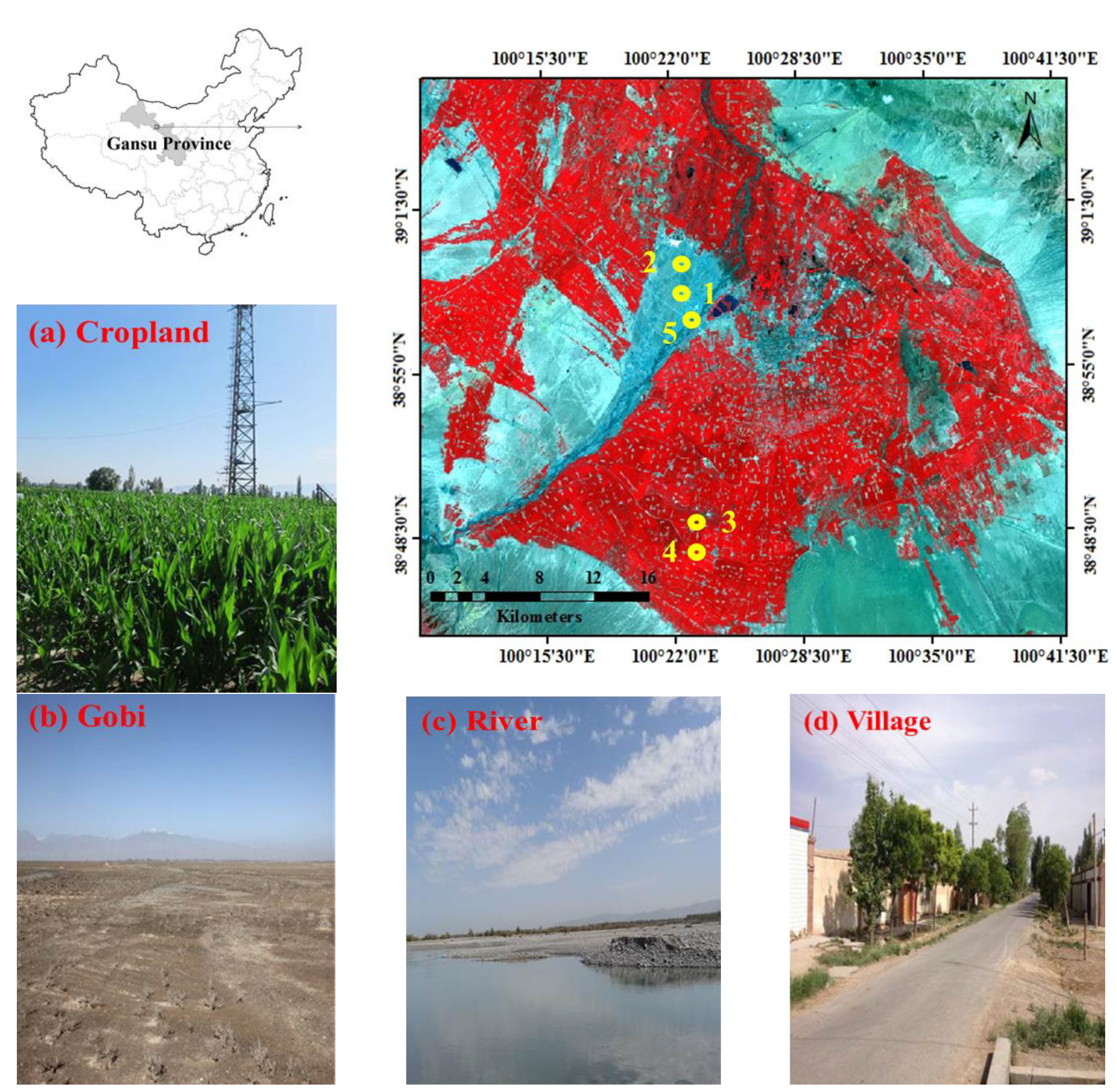
HiWATER is an ongoing watershed-scale eco-hydrological experiment designed from an interdisciplinary perspective to address problems that include heterogeneity, scaling, uncertainty and closing of the water cycle at the watershed scale. The experiment was performed in the Heihe River Basin, which is in the arid region of northwestern China (Gansu Province) between 97.1°E–102.0°E and 37.7°N–42.7°N. Three Key Experimental Areas (KEAs) were selected to conduct intensive and long-term observations: the cold region experimental area in the upper reaches, the artificial oasis experimental area in the middle reaches, and the natural oasis experimental area in the downstream region [19,20]. The airborne and satellite-based observations in this study were derived simultaneously from the KEA of the middle stream at approximately 12:00 am (local time) on 10 July 2012.

2.2. Study Regions

Four main types of land cover are present in the middle-stream KEA: cropland, village, Gobi and river. The cropland accounts for more than half of the TASI data used in this study and consists of large areas of corn and some wheat. The village is composed of houses and small roads. The Gobi land cover consists of small gravel, bare soil and small areas of Alhagi sparsifolia Shap., which is a spiny, perennial subshrub that grows mainly in saline and arid regions in the native ranges of northwestern China, Central Asia, India, and the Middle and Near East [19]. A small branch of the Heihe River is present in the Gobi land. Within these four land surface types, five study areas (1260 m × 2880 m) were selected, including two Gobi areas, two areas of cropland mixed with villages, and one Gobi area that contained the river. Ground photographs of the four land cover types and the geographical locations of these study regions are shown in Figure 1.
The land cover types in these regions were derived from a dataset, which is composed of the classification results of HJ-1/CCD data on a monthly basis (Table 1) [21,22]. The classification data in July, 2012 was selected. Based on the validation data from the ground measurements and high-resolution data, the classification accuracy is 93.06%, and the Kappa coefficient is 0.92. The main land surface types, average LST values and their standard deviations are summarized in Table 2. The different standard deviations of these five study areas indicate that the spatial heterogeneity increases from the Gobi areas to the cropland areas to the mixed Gobi and river area. These differences provide the range of spatial heterogeneity that is necessary for this study.
Table 1. Percentages of the four land cover types in the five study regions. These results are derived from the classification of HJ-1/CCD data. The Gobi and bare soil in the cropland are not distinguished in this classification scheme.
SitesVegetation (%)Water (%)Village (%)Gobi/Bare Soil (%)
Site 100.9673099.0327
Site 20.14880099.8512
Site 395.535704.11710.3472
Site 496.279803.62100.0992
Site 59.17626.43850.148864.2361
Figure 1. Spatial distribution and ground photographs of the five study sites. The upper right image is the ASTER L1 B VNIR image of the study area taken on 10 July 2012. The RGB components are channels 3 (0.81 μm ), 2 (0.66 μm ) and 1 (0.56 μm ), and the spatial resolution is 15 m. The land cover types include (a) cropland, (b) Gobi, (c) river and (d) village.
Remotesensing 07 06489 g001
Table 2. The main types of land surface cover and the mean values and standard deviations of LST in the five study areas. mLST and σLST represent the mean and standard deviation, respectively, and were calculated from both the ASTER and TASI LST images.
SitesLand Surface TypemLST (K) (ASTER)mLST (K) (TASI)σLST (K) (ASTER)σLST (K) (TASI)
Site 1Gobi321.04321.071.242.29
Site 2Gobi320.12319.971.642.44
Site 3Vegetation303.73304.492.365.19
Site 4Vegetation303.11303.832.355.01
Site 5Mixed313.81313.815.338.62

2.3. Experimental Data Preprocessing

TASI airborne data and ASTER satellite data collected during the HiWATER experiment were used in this study. The data were acquired at nearly the same time; thus, the temporal difference between the datasets was neglected. The image registration between the TASI and ASTER data was performed using the georegistration information in the images, which can reach an accuracy of 1.5 m.

2.3.1. Description and Preprocessing of ASTER Data

ASTER was launched on NASA’s Terra satellite in December 1999. The thermal infrared (TIR) sensor of ASTER is a five-band nadir viewing scanner (±3°) that is pointable to ±8.5° and has a 90 m spatial resolution and a 63 km wide swath [6,17]. The overpass time of the ASTER data used in this study is 00:13 pm (local time) on 10 July 2012.
The ASTER L1B products were used to estimate the LST from the ASTER data using the TES algorithm [23]. The atmospheric correction was performed using the radiative transfer model of MODTRAN with input atmospheric profiles generated by the National Center for Environmental Prediction (NCEP). The waveband integrated values of three atmospheric radiative property parameters, including transmittance, upwelling and downwelling radiance, were acquired from the MODTRAN calculations. The Water Vapor Scaling (WVS) algorithm [24] was utilized in the correction process to improve the performance of the atmospheric correction. The surface outgoing radiance was then derived from the at-sensor radiance using the radiative transfer function:
L s u r , i = L s e n , i   L a t m , i   τ a t m , i =   ε i B i ( T s ) + ( 1 ε i )   L a t m , i  
where i is the band, L s u r , i is the surface outgoing radiance, L s e n , i is the observed radiance, L a t m , i   is the upwelling atmospheric radiance, τ a t m , i is the transmissivity, ε i is the surface emissivity, B i ( T s ) is the Planck radiance, T s   is the LST, and L a t m , i   is the downwelling atmospheric radiance.

2.3.2. Description and Preprocessing of TASI Data

TASI is a new generation of commercial hyperspectral infrared sensor that was released by ITRES of Canada in 2006. TASI is designed to detect land surface temperature and emissivity characteristics and has 32 bands in the TIR region (8–11.5 μm ) of the electromagnetic spectrum, a wavelength spacing of 0.1095 μm , a full width at half maximum (FWHM) of 0.0548 μm , and a total field of view of 40° at a spatial resolution of 3 m [25].
To be consistent with the acquisition time of the ASTER data, the slice of TASI data began at 00:14 pm (local time) on 10 July 2012, and ended at 00:22 pm (local time). The flight duration was 8 min, during which the LST was assumed to be stable. In this case, the temporal effect was negligible.
The preprocessing of the TASI data included three main steps: radiometric calibration, geometric correction and atmospheric correction. The first two steps were completed by the software provided by ITRES. In this study, the In-Scene Atmospheric Compensation (ISAC) algorithm was used to perform the atmospheric correction [26].
Based on the TES algorithm for the ASTER data, a modified TES algorithm for the TASI data was proposed to derive the LST and spectral emissivities. The inversion result was validated by a root mean square error (RMSE) of approximately 1.3 K for temperature. The emissivity spectrum was very similar to that of the field measurements from a Bomem Fourier transform infrared (FTIR) spectrometer [25].

3. Methodology

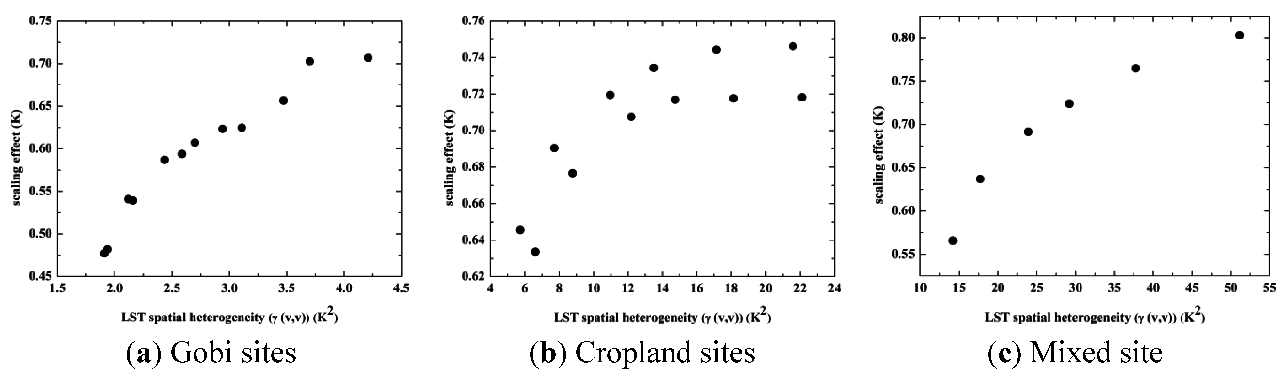
3.1. Quantification of the Spatial Heterogeneity of LST

The spatial heterogeneity of LST should be quantified to analyze the scaling problem [8,11]. In this study, the dispersion variance was used as a quantifiable parameter to describe the LST’s spatial heterogeneity by integrating the fitted variogram over a spatial scale. The calculation process followed two steps. First, a variogram describing the correlation between neighboring sites as a function of the spatial separation [18] was fitted to the LST data using the semi-automatic fitting software Isatis in a probabilistic framework. The dispersion variance was then calculated as follows:
  γ ( v , v ) =   1 | v | 2 x v , y v γ ( | x y | ) d x d y
where γ ( v , v ) is the dispersion variance; γ ( | x y | ) is the fitted variogram; | x y | represents the distance between two LST points, which are denoted as x and y in domain v and | v | represents the area of v .
A variogram was fitted to the estimated LST in each study regions. Because of the loss in the spatial heterogeneity of the data at coarse resolution [18], the variograms in the five regions were fitted with the TASI LST data rather than with the ASTER LST data.

3.2. Methods of Studying the LST Scaling Problem

The two aspects of the LST scaling problem were studied by comparing the remotely sensed LST products in two ways. First, the LST products calculated at the pixel resolution and upscaled to coarser scale using upscaling methods were compared with the products calculated at a coarse resolution by aggregating the fine-resolution data to the coarse data. Second, the TASI and ASTER LST products, both derived from the TES algorithm, were compared. The two methods of comparison were used to investigate the two aspects of the LST scaling problem.

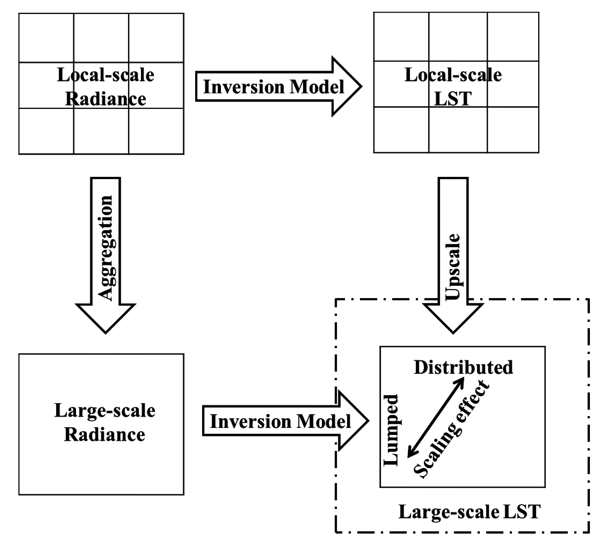
3.2.1. Comparison between Distributed LST and Lumped LST

Figure 2 shows a schematic of the first comparison. Two methods were developed to acquire the LST products at large scale with the same sensor: the distributed method and the lumped method. In the distributed method, the LST product was calculated at the pixel resolution by the TES algorithm and upscaled to a coarse scale. In the lumped method, the radiance data were first aggregated to the coarse scale based on the law of energy conservation, and the LST was then calculated with the coarse data using the TES algorithm. Four different methods were used in the LST upscaling process [11]. Because the study areas are very flat, the relief effect was not considered in the four upscaling methods. Combined with the S-B law and irradiance average theory, the large-scale LST was computed from the small-scale LST as follows:
T =   ( r i ε i T i 4 ε r i ) 1 / 4
where the subscript i denotes pixel i ; ε i and T i are the BBE and the LST at the small scale, respectively; r i is the areal ratio of the small-scale grid spacing i within the large-scale spacing, it equals 1 for the small-scale grid spacing within the large-scale spacing; and ε is the BBE for the large-scale pixel. The narrow band emissivities were estimated using the TES algorithm. The BBE for the ASTER data was estimated from the narrow band emissivities based on the linear equation provided by Cheng et al. [27]. For the BBE of the TASI data, the emissivity spectrum was first transformed to the five TIR bands of ASTER with the spectral response function of ASTER, and the BBE was then calculated using the same equation as for the ASTER BBE. Based on Zhang et al. [28], ε was derived from ε i   with the areally weighted averaging approach. The large-scale LST is determined by the LST and the emissivity at the local scale, as well as the emissivity at the large scale. When the emissivity is neglected, Equation (3) becomes
  T =   ( r i T i 4 r i ) 1 / 4  
where the LST at the large scale is only affected by the fine-resolution LST and their areal ratio. If the exponent is eliminated, Equation (3) becomes
  T =   r i ε i T i ε r i   .  
If the surface emissivity is neglected, it becomes
T =   r i T i r i   .
The upscaling methods described by Equations (3–6) are denoted as Method 1, Method 2, Method 3, and Method 4, respectively. Correspondingly, the distributed LSTs upscaled by the equations are denoted as L S T m 1 d i s t r i b u t e d , L S T m 2 d i s t r i b u t e d   L S T m 3 d i s t r i b u t e d and L S T m 4 d i s t r i b u t e d , respectively.
A rectified method of LST estimation was developed to acquire the effective LST at large scales based on the TES algorithm. The emissivity used to retrieve the LST at large scales was estimated by aggregating the emissivity derived from the original data by the TES algorithm instead of calculating it with the TES algorithm at coarse resolutions [28]. The LST was then calculated in the same way as the TES algorithm with the aggregated emissivity. This rectified LST is virtually the ensemble radiometric temperature calculated with the ensemble r-emissivity, which was defined by Norman et al. [29]. In this case, the rectified LST can be viewed as the effective LST at large scales.
The difference between the lumped LST and the distributed LST is defined as the scaling effect, which is expressed as
  e s c a l i n g =   L S T l u m p e d L S T d i s t r i b u t e d  
where e s c a l i n g is the scaling effect, L S T l u m p e d is the lumped LST, and L S T d i s t r i b u t e d is the distributed LST. To measure the scaling effect at a given spatial resolution for a specific study site, the mean scaling effect is introduced as
  e s c a l i n g m e a n =   1 N   i = 1 N | L S T i l u m p e d L S T i d i s t r i b u t e d   |
where N is the total number of large-scale pixels in the study area; and L S T i l u m p e d and L S T i d i s t r i b u t e d   are the ith LST pixels in the study area derived from the lumped method and the distributed method, respectively.
Figure 2. Schematic of the comparison between the distributed and lumped LSTs. The same inversion model is used in the distributed method and the lumped method.
Remotesensing 07 06489 g002

3.2.2. Comparison between the TASI and ASTER LSTs

In this study, the TASI and ASTER LSTs were both retrieved with the TES algorithm to eliminate the inconsistency of the retrieval algorithm. To analyze the factors that account for the scaling uncertainties, the TASI and ASTER LSTs were compared in the study regions.

3.3. Correction Methodology for the LST Scaling Effect

In this study, we assumed the distributed LST to be the accurate effective temperature on a large scale. To ensure consistency between the LSTs estimated from the distributed and lumped methods, corrections should be performed on the lumped LST. The empirical relationship between the emissivity and the spectral contrast in the TES algorithm may cause biases in the estimated LST [17]. Based on the approach developed by Hu and Islam [2], we proposed a scaling error correction model to correct this relationship
ε m i n = a b . M M D c
where ε m i n is the minimum emissivity in the emissivity spectrum; a , b and c are the three regression coefficients; and M M D denotes the maximum-minimum emissivity difference among the normalized emissivity spectrum and represents the spectral contrast. By assuming that (i) the M M D values vary slowly, (ii) the relationship is continuous and weakly nonlinear, and (iii) continuous derivatives of the relationship exist at least up to the second order, the relationship was corrected by a second-order Taylor series expansion as follows:
ε m i n = a b . M M D c +   f ( M M D ) . s 2 / 2
where f ( M M D ) is the second derivative of the original empirical relationship (Equation (9)) and s 2 is the local variance of the M M D . The M M D at large scale was calculated by inputting the aggregated radiance into the TES algorithm, of which the scaling effect was not considered. The lumped LST was then retrieved using this corrected TES algorithm.

4. Results and Discussion

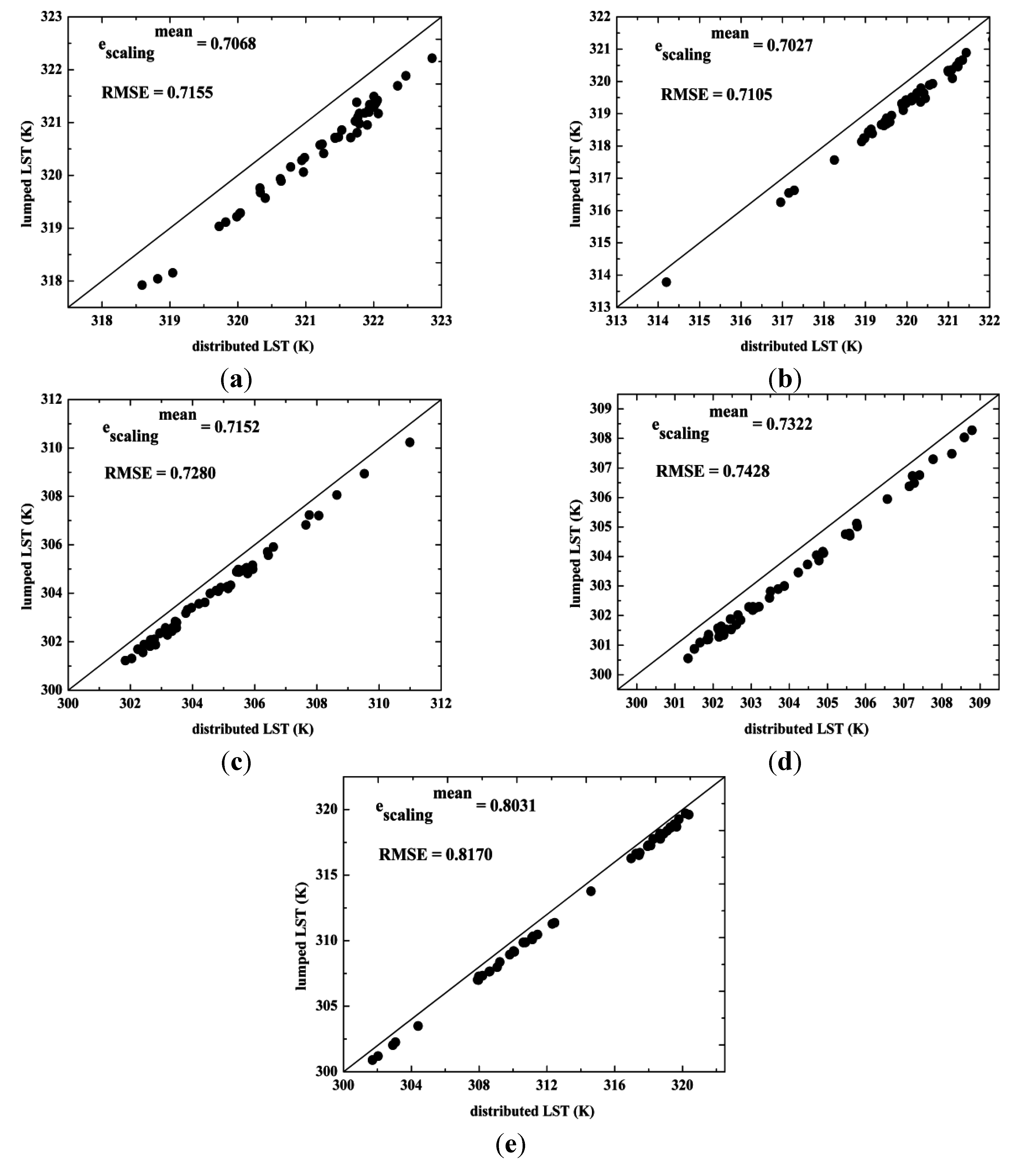
4.1. Analysis of the Comparison between the Distributed LST and the Lumped LST

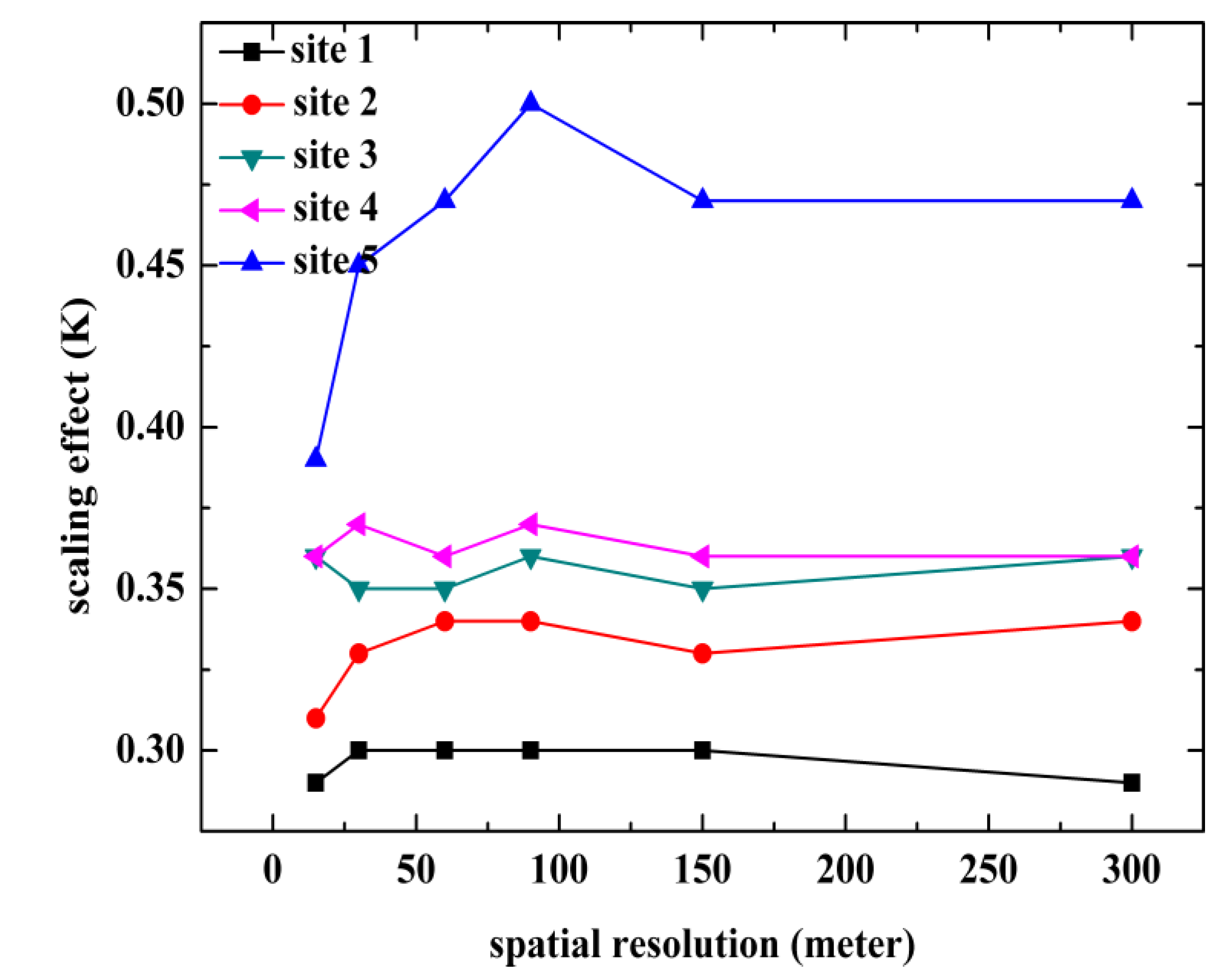
4.1.1. Analysis of the TASI LST Data

In the analysis, the distributed LST is viewed as the effective LST at large scales. The rationality of this assumption will be demonstrated in the subsequent experiment. Four upscaling methods were used to estimate the distributed LST; as a result, four different graphs of the scaling effects that were calculated with Equation (8) were acquired (Figure 3). The scaling effects of Methods 1 and 2 are similar, and the scaling effects of Methods 3 and 4 are similar. Thus, the following analyses are divided into two groups (Methods 1–2 vs. Methods 3–4). The purpose of the comparison is to investigate the first aspect of the LST scaling problem. The key to the TES algorithm is the empirical relationship between the emissivity values and the spectral contrast [23]. The laboratory samples used to calibrate the TES’s empirical relationship are homogeneous. When the spatial resolutions of the remotely sensed data are fine (e.g., 3 m), the TES algorithm can be applied successfully. When the data are coarse, the significant differences between the laboratory measurements and the coarse data may induce significant errors in the LST estimation [17].
In Method 1 and Method 2, the scaling effects initially increase with the spatial resolution and then become asymptotic. This behavior can be explained by the saturation of heterogeneity. An investigation of spatial heterogeneity [18,30] showed that the heterogeneity increases as the spatial resolution becomes larger until the scale approaches the characteristic scale of the landscape. The uncertainty of the empirical relationship in the TES algorithm is affected by the spatial heterogeneity. In this case, the scaling effect is closely related to the spatial heterogeneity; thus, it becomes saturated when the spatial resolution reaches the characteristic scale. Three types of study areas with different characteristic scales were selected in this study. Correspondingly, the scaling effect becomes asymptotic at these distinctive spatial scales. The spatial heterogeneity increases from Gobi land to cropland to the mixed area. Under these circumstances, the scaling effects in the Gobi sites are the smallest at all scales, where they have a maximum of 0.7 K, and they are greater in cropland, where they reach a maximum of 0.75 K. The scaling effect at Site 5 is less than at the cropland sites when the spatial resolution is less than approximately 110 m, but it exceeds the scaling effect at the cropland sites when the spatial resolution is larger. This pattern occurs because Site 5 is a mixed area of Gobi, cropland and river. When the spatial resolution is fine, the number of mixed pixels in the landscape is small and the mean scaling effect is small; when the spatial resolution is coarse, mixed pixels with different land cover types make up a larger proportion of pixels; thus, the mean scaling effect increases because of the greater heterogeneity. In general, the rules of change for the scaling effect in Method 1 and Method 2 are nearly identical.
Figure 3. Relationship between the spatial resolution and the LST scaling effect. The distributed LSTs are acquired from (a) Method 1; (b) Method 2; (c) Method 3 and (d) Method 4.
Remotesensing 07 06489 g003
In Methods 3 and 4, the relationships between the spatial resolution and the scaling effect at Site 1 and Site 2 are similar to those in Methods 1 and 2. The relationships are different for Sites 3–5, especially at large scales. The difference is inferred to be caused by the upscaling methods. In this study, the upscaled LST is considered to be the accurate LST; its accuracy determines the subsequent analysis of the scaling effect. In contrast to Methods 1 and 2, Methods 3 and 4 neglect the exponent in the upscaling process, which may cause errors in the upscaled LST when the land surface heterogeneity is significant. The land surfaces at Sites 1 and 2 are relatively homogeneous compared with the other sites; thus, neglecting the exponent in the upscaling process does not significantly affect the accuracy of the upscaled LST. The land surfaces at the other three sites are heterogeneous, and neglecting the exponent will cause a large upscaling bias. The smaller scaling effects at Sites 3–5 for Methods 3 and 4 are notable. This difference is attributed to the underestimated distributed LST values with Methods 3 and 4 in these areas compared to Methods 1 and 2 (Table 3). The means at Sites 3–5 are lower by approximately 0.15 K when they are upscaled by Methods 3 and 4 than when they are upscaled by Methods 1 and 2. Because the lumped LST values are generally smaller than the distributed LST values (Figure 4), the difference between the distributed and lumped LSTs decreases when the distributed LST is underestimated, which accounts for the decreasing scaling effect.
The LST estimated using the rectified method and the distributed LST were compared to ensure that the distributed LST is the effective LST at large scales. The comparison result is shown in Figure 5. The distributed LSTs estimated from Methods 1 and 2 are nearly the same as the rectified LST, which proves the assumption described at the beginning of this section that the distributed LST should be viewed as the effective LST rather than the lumped LST. The biases in Method 1 are slightly smaller than those in Method 2. In Methods 3 and 4, the biases are also negligible at Sites 1 and 2, whereas the biases at Sites 3–5 are significant, especially when the spatial scale is greater than 100 m. This result corresponds to the inference that the distributed LST values with Methods 1 and 2 are more effective than those with Methods 3 and 4, especially when the spatial heterogeneity is significant. Additionally, this result ensures that the scaling effect in the TES algorithm is mainly attributed to the empirical relationship between the emissivity values and the spectral contrast.
The analysis presented above demonstrates that the TES algorithm will cause a bias in the retrieved LST at large scales because of the inconsistency between the laboratory measurements and the large-scale data, which directly affects the estimated emissivity. Methods 1 and 2 can upscale the LST more effectively than Methods 3 and 4.
Table 3. Statistics of the distributed TASI LST (300 m) from four different upscaling methods in terms of the minimum, maximum and mean LST values at the five sites. Methods 1–4 are labeled as M1–M4, respectively.
LST at Site 1 (K)LST at Site 2 (K)LST at Site 3 (K)
Min.Max.MeanMin.Max.MeanMin.Max.Mean
M1318.59322.86321.26314.20322.07319.77301.84310.99304.69
M2318.59322.86321.26314.23322.08319.78301.85311.02304.71
M3318.56322.85321.24314.09322.06319.75301.81310.72304.57
M4318.57322.86321.24314.13322.07319.76301.82310.75304.58
LST at Site 4 (K)LST at Site 5 (K)
Min.Max.MeanMin.Max.Mean
M1301.34308.79304.08301.71320.37313.55
M2301.35308.79304.09301.76320.38313.57
M3301.34308.49303.96301.31320.35313.30
M4301.34308.49303.97301.36320.35313.33
Figure 4 shows a pixel-by-pixel comparison between the distributed LST upscaled using Method 1 and the lumped LST for the five study areas at a spatial resolution of 300 m. The lumped LST is underestimated in all of the areas. The scaling effects and RMSEs at Sites 1–4 are similar (approximately 0.7 K), which is also reflected in Figure 3 (at a resolution of 300 m in Figure 3a). The similarity is attributed to the saturated scaling effect at the spatial scale of 300 m. The scaling effect and RMSE at Site 5 are obviously larger than those at the other sites (approximately 0.8 K) because of the large heterogeneity in the mixed area.
Scatter plots between the spatial heterogeneity and the scaling effect for the five study sites are shown in Figure 6. The scaling effect is proportional to the intra-pixel heterogeneity, which is quantified by the dispersion variance γ ( v , v ) , at all the sites. As the dispersion variance increases, the scaling effect becomes more notable.
Figure 4. Pixel-by-pixel comparison of the distributed LST (with Method 1) and the lumped LST (300 m) at (a) Site 1, (b) Site 2, (c) Site 3, (d) Site 4 and (e) Site 5.
Remotesensing 07 06489 g004
Figure 5. Comparison between the rectified TASI LST and the distributed LST by (a) Method 1; (b) Method 2; (c) Method 3 and (d) Method 4. The difference is described by the mean absolute bias in the LST image (Equation (8)).
Remotesensing 07 06489 g005
Figure 6. The relationship between spatial heterogeneity of the LST quantified by the dispersion variance γ ( v , v ) and the scaling effect in (a) the sites covered by Gobi (Sites 1 and 2); (b) the sites covered by cropland (Sites 3 and 4); and (c) the mixed site (Site 5).
Remotesensing 07 06489 g006
In conclusion, the scaling effect is largest in the mixed area of Site 5, which is the most heterogeneous site at the landscape level, and is moderate at the cropland sites and smallest at the most homogeneous Gobi sites. The scaling effect increases rapidly with the spatial resolution until the resolution reaches the characteristic scale of the landscape, and the scaling has a positive correlation with the spatial heterogeneity, which is quantified by the dispersion variance.

4.1.2. Analysis of the ASTER LST Data

The ASTER LST scaling effect is described in Figure 7. Because the results from upscaling Methods 1 and 2 are nearly the same, only the results from Method 1 are shown. The scaling effect is not significant for the ASTER data. The largest scaling error at all scales at all of the study sites is only 0.06 K, and the range of the scaling effect is 0.003–0.06 K, which can nearly be neglected. The scaling effect does not increase with the spatial scale; it remains nearly constant for all spatial scales. This quasi-constant scaling effect can be attributed to the significant spatial heterogeneity in the 90-m ASTER pixels. Because of the heterogeneity in the ASTER data, there is an inconsistency between the laboratory measurements and the satellite data that causes a bias in the empirical relationship when it is used to estimate the emissivity at a spatial resolution of 90 m. The bias propagates to the estimated LST. The bias is still present when the TES algorithm is used at larger scales and it does not increase significantly. Thus, the biases in the distributed and lumped ASTER LSTs cancel each other out in the calculation of the scaling effect.
It should be noted that our purpose is not to prove the ineffectiveness of the TES algorithm. When the aim is to retrieve an LST product with an accuracy of 1 K or higher, the scaling effect in the TES algorithm should be considered.
Figure 7. The relationship between the spatial resolution and the LST scaling effect for the ASTER LST data in the five study areas. The distributed LST was derived from Method 1.
Remotesensing 07 06489 g007

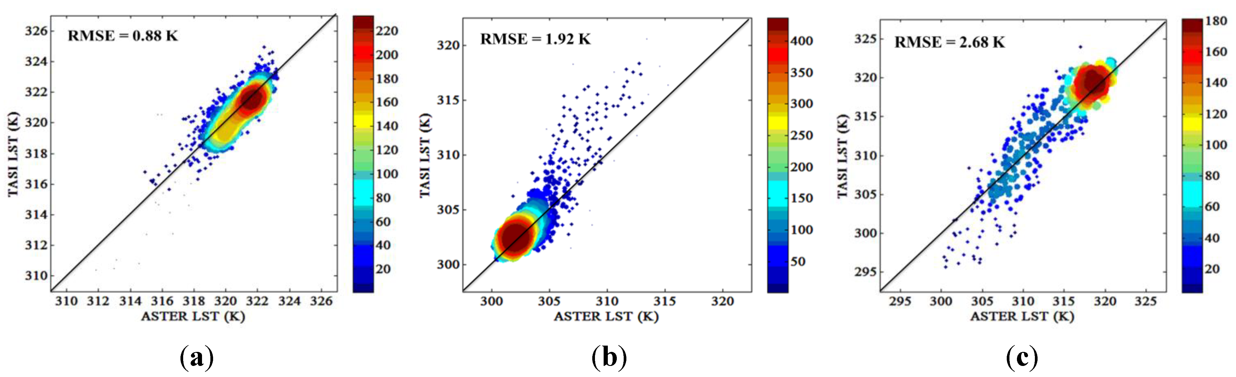
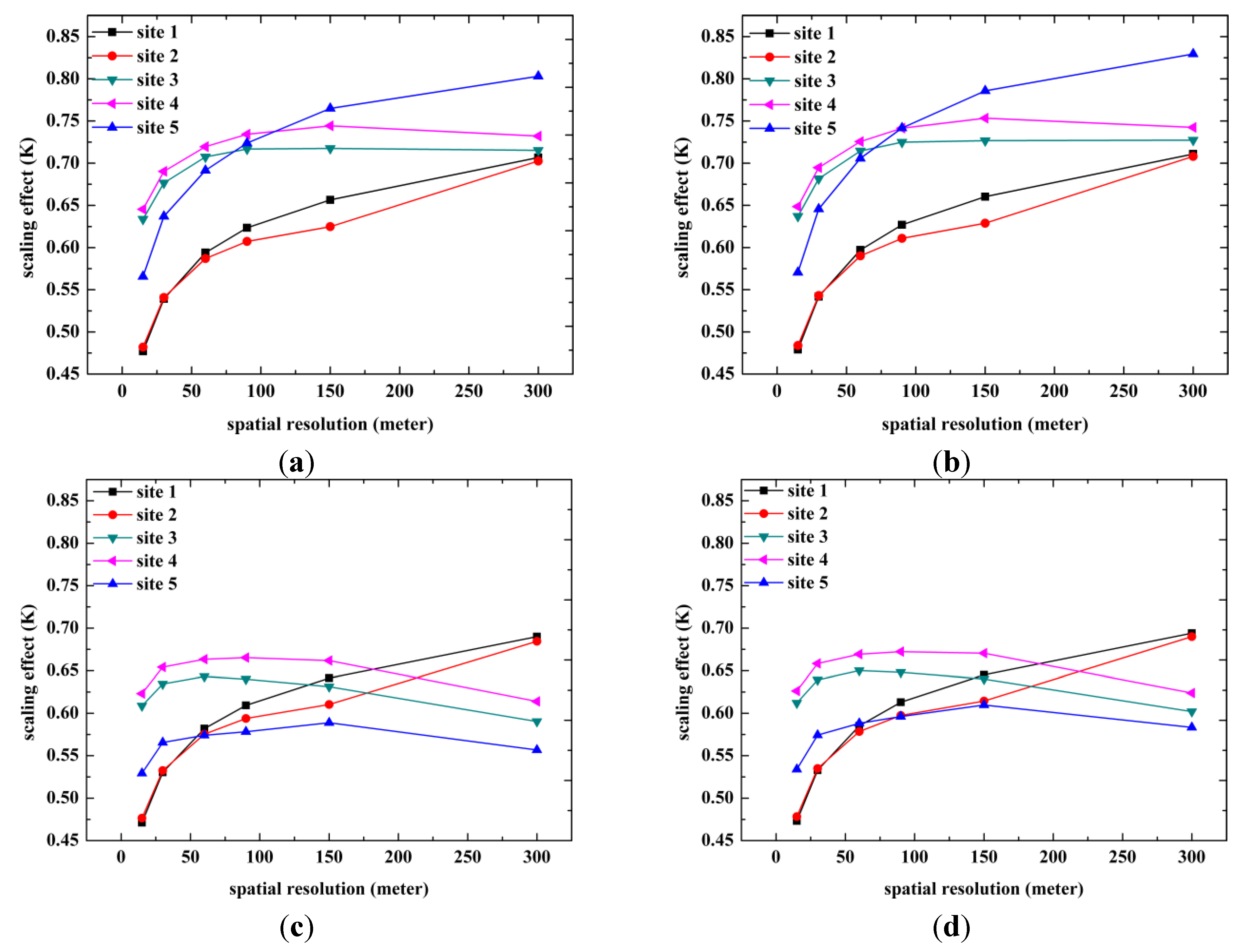
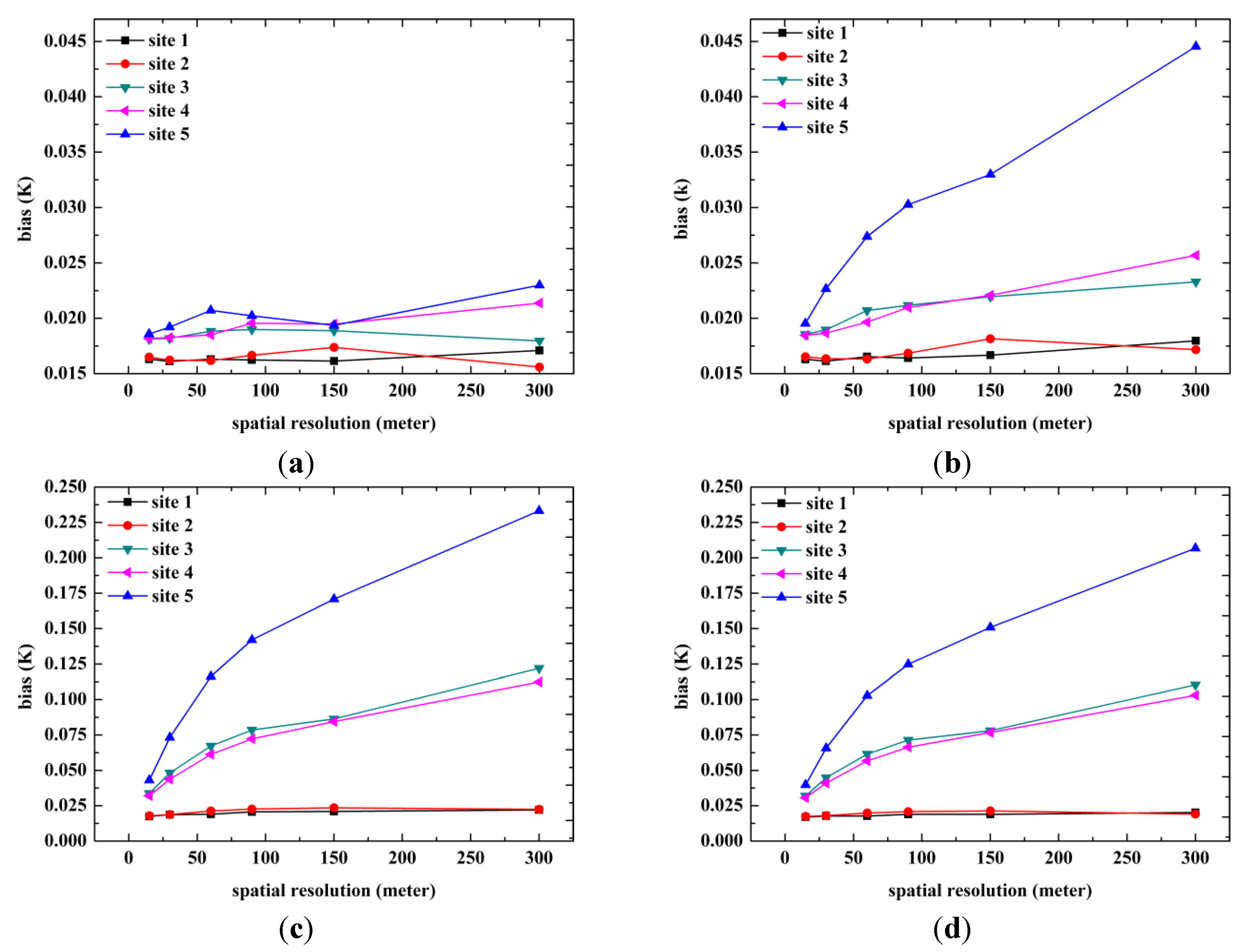
4.2. Analysis of the Comparison between the ASTER and TASI LSTs

To investigate the relationship between the ASTER LST data and the TASI LST data, the TASI LST data were upscaled to the spatial resolution of the ASTER LST data. The RMSEs between the ASTER LST and the distributed TASI LST derived by Methods 1 and 2 are shown in Table 4. Because of the upscaling biases in Methods 3 and 4, these methods were not used to decrease the uncertainty caused by the upscaling method. The RMSE values in Method 1 and Method 2 were nearly the same in all five study regions. The differences between the ASTER and TASI LSTs are closely related to the land cover types. In the sites covered by Gobi, the RMSEs were both approximately 0.9 K. In the sites covered by cropland, the RMSEs were slightly greater than 1.9 K. In the mixed site, the RMSE reached 2.68 K. The comparisons between the ASTER and TASI LSTs over different land covers are shown in Figure 8. Most of the points cluster on the 1:1 line, which indicates a good consistency between the ASTER and TASI LST. The LST points in the Gobi areas cluster between 319 K and 322 K on the 1:1 line because of the high temperatures at the Gobi sites. Numerous points cluster on the 1:1 line between 300 K and 305 K because of the relatively lower temperatures in the cropland sites. The mixed area is the most heterogeneous; accordingly, the points cluster in a larger range between 315 K and 322 K on the 1:1 line. The points in Figure 8a are the most clustered because of the homogeneity in the Gobi regions, whereas the points are the most dispersed in Figure 8c because of the significant heterogeneity of the mixed site.
Table 4. RMSE values between the ASTER and distributed TASI LSTs. The distributed LSTs are upscaled by Methods 1–4. The RMSEs in Sites 1–5 are labeled as RMSE1–RMSE5, respectively.
RMSE1 (K)RMSE2 (K)RMSE3 (K)RMSE4 (K)RMSE5 (K)
Method 10.810.951.931.912.68
Method 20.810.951.941.922.68
Figure 8. Comparison between the ASTER LST data and the TASI LST data in (a) Gobi areas; (b) cropland areas and (c) the mixed area. The TASI LSTs were upscaled using Method 1. The sizes of the dots in the scatterplots correspond to their density in the swarm of points. The larger dots are given hotter colors in the dense particle region.
Remotesensing 07 06489 g008
The inconsistency between the ASTER and TASI LSTs can be attributed to the land surface heterogeneity and the limited accuracy in the retrieved LST products. The more significant the spatial heterogeneity of the study site, the greater the RMSE; this pattern reflects the close relationship between the spatial heterogeneity and the inconsistency. The TES algorithm was used to estimate the LSTs for both the TASI and the ASTER data. However, the accuracy of the TES algorithm is affected by the atmospheric correction errors of the images, especially over gray bodies [31]. The WVS algorithm was used to refine the atmospheric correction for the ASTER data, whereas the ISAC algorithm was used to correct the atmospheric effect. The two different atmospheric corrections can greatly affect the accuracy of the products. Additionally, the different spatial scales of the ASTER and TASI data can cause different uncertainties in the empirical relationship between the emissivity values and the spectral contrast, which affects the retrieved LST.

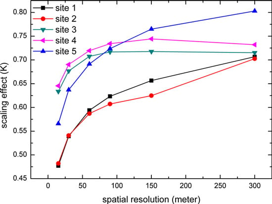
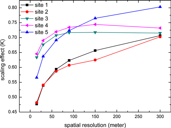
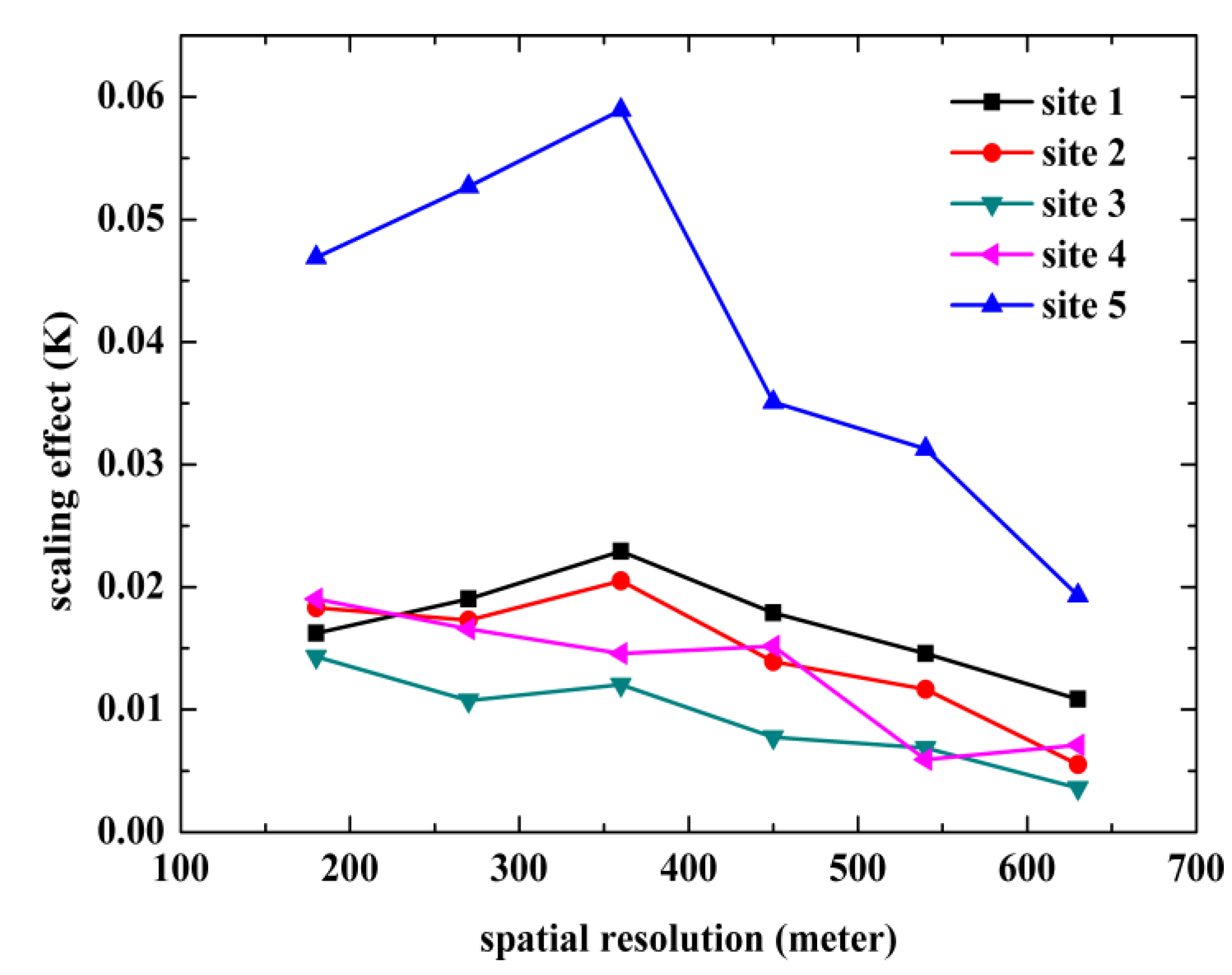
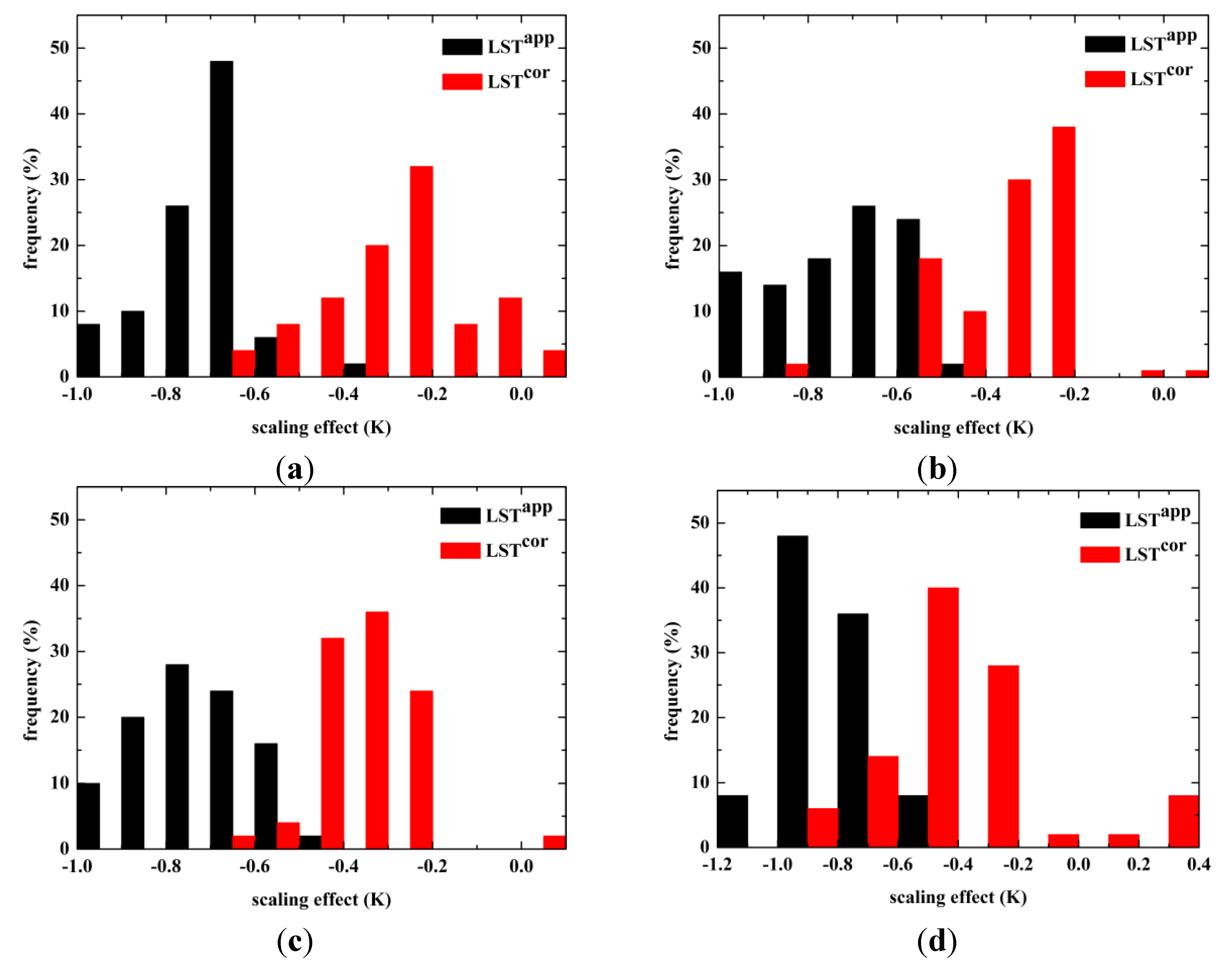
4.3. Correcting the Scaling Effect

Because of the significant scaling effect of the TASI LST data, the scaling effect was corrected with a scale-transformation model based on a Taylor expansion (Figure 9). The scaling effect after the scaling correction decrease in the five study regions and are always less than 0.5 K. The scaling effects in the more heterogeneous sites are still greater than in the relatively homogeneous sites after the correction. Additionally, the correction provided resolution-invariant results for the scaling effect.
The correction results for Site 1, Site 3, Site 4 and Site 5 at a spatial scale of 300 m are shown in Figure 10. Because of the similar pattern of scaling effect at Site 2 with that at Site 1, the result at Site 2 is not shown. The distributed LSTs were upscaled using Method 1. The proportion of pixels with a large scaling effect clearly decreases, whereas the proportion of pixels with a slight scaling effect increases. The peaks move from large scaling effect values to smaller values. The peaks move from −0.7 K to −0.3 K and from −0.7 K to −0.4 K for Site 1 and Site 2, from −0.7 K to −0.3 K and from −0.8 K to −0.4 K for Site 3 and Site 4. For Site 5, the peak moves from −1.0 K to −0.5 K.
Figure 9. Relationship between the spatial resolution and the LST scaling effect after the scaling correction. The distributed LSTs were upscaled using Method 1.
Remotesensing 07 06489 g009
Figure 10. Histograms of the difference between the distributed LST and lumped LST before and after the scaling effect correction at (a) Site 1; (b) Site 3; (c) Site 4 and (d) Site 5 at a spatial scale of 300 m. The black bars ( L S T a p p ) represent the frequencies of the scaling effect before the correction, and the red bars ( L S T c o r ) represent the frequencies of the scaling effect after the correction.
Remotesensing 07 06489 g010

5. Conclusions

The goal of this study was to investigate the scaling problem of LST. Five areas were selected for study using simultaneous multi-sensor observations from the HiWATER experiment. Sites 1 and 2 are Gobi areas, Sites 3 and 4 are cropland areas, and Site 5 is a mixed area of Gobi and water. The LST’s spatial heterogeneity increases from the Gobi areas to the cropland areas to the mixed area. The multi-sensor data included airborne TASI data and satellite ASTER data. The data were acquired at nearly the same time; thus, the temporal change of the LST data was not taken into consideration. The LSTs for the ASTER and TASI data were both retrieved using the TES algorithm. To describe the spatial heterogeneity of the LSTs at the landscape level in the study areas, the dispersion variance was estimated based on variogram modeling.
The LST data were upscaled to coarser resolutions according to four different upscaling methods based on the S-B law and were compared to investigate the relationship between the spatial resolution and the scaling effect. Methods 1 and 2 provide similar results, and Methods 3 and 4 provide similar results. Additionally, the nearly identical results of the upscaled TASI LSTs from the first two methods and the rectified TASI LSTs indicate that Methods 1 and 2 can accurately upscale fine-resolution LST data, which is because of the conservation of the exponent relationship in the S-B law in Methods 1 and 2.
The scaling effect of the TASI LST data is clear and could be as large as 0.8 K. This effect increases with the spatial resolution until the spatial resolution reaches the characteristic scale of the study area. The scaling effect is greatest in the mixed area of Site 5, which is the most heterogeneous site at the landscape level, and is moderate for cropland sites and smallest for the most homogeneous Gobi sites. The scaling effect of the ASTER LST data is not significant and had a maximum of 0.06 K. This finding may be caused by the significant heterogeneity in the original ASTER pixels. The comparison between the TASI data and the ASTER data showed that they were highly consistent, with a RMSE of approximately 0.88 K, when the pixels were relatively homogeneous. When the spatial heterogeneity was significant, the RMSE could be as large as 2.68 K. A scale-correction model based on a Taylor expansion was developed based on the analysis of scaling effect. In this model, the scaling effect caused by the nonlinear relationship between the MMD and the radiance was not considered. The scaling-correction methodology showed that the scaling effect was resolution invariant and was always less than 0.5 K, which demonstrates the effectiveness of the scaling-correction methodology.
Because of the limited spatial range of the data, the conclusions in this study may not be generalized; this would require a larger database and a more detailed analysis. However, this study provides useful insights into the scaling problem of LST.

Acknowledgments

All of the data used in this study were obtained from the HiWATER experiment. We thank all of the scientists and engineers who participated in this campaign. We thank the anonymous reviewers for their helpful comments and suggestions that have significantly improved this article. This work was supported in part by Chinese Natural Science Foundation Project (91125003), National Basic Research Program of China (2013CB733401), National High-Technology Research and Development Program of China (863 Project: 2012AA12A304), Chinese Natural Science Foundation Project (41101325, 41171282) and Chinese Academy of Sciences Action Plan for West Development Project (KZCX2-XB3-15).

Author Contributions

Tian Hu and Qinhuo Liu conceived the study topic and the research methodology; Tian Hu and Heshun Wang selected the study areas and processed the data; Tian Hu, Qinhuo Liu, Yongming Du, Hua Li and Biao Cao analyzed the result; and Tian Hu wrote the paper.

Conflicts of Interest

The authors declare no conflict of interest.

References

  1. Raffy, M. Change of scale in models of remote sensing: A general method for spatialization of models. Remote Sens. Environ. 1992, 40, 101–112. [Google Scholar] [CrossRef]
  2. Zhenglin, H.; Islam, S. A framework for analyzing and designing scale invariant remote sensing algorithms. IEEE Trans. Geosci. Remote Sens. 1997, 35, 747–755. [Google Scholar] [CrossRef]
  3. Garrigues, S.; Allard, D.; Baret, F.; Weiss, M. Influence of landscape spatial heterogeneity on the non-linear estimation of leaf area index from moderate spatial resolution remote sensing data. Remote Sens. Environ. 2006, 105, 286–298. [Google Scholar] [CrossRef]
  4. Chen, J.M.; Chen, X.; Ju, W. Effects of vegetation heterogeneity and surface topography on spatial scaling of net primary productivity. Biogeosciences 2013, 10, 4879–4896. [Google Scholar] [CrossRef]
  5. Moran, M.; Humes, K.S.; Pinter, P.J., Jr. The scaling characteristics of remotely-sensed variables for sparsely-vegetated heterogeneous landscapes. J. Hydrol. 1997, 190, 337–362. [Google Scholar] [CrossRef]
  6. Hulley, G.C.; Hook, S.J. Generating consistent land surface temperature and emissivity products between aster and modis data for earth science research. IEEE Trans. Geosci. Remote Sens. 2011, 49, 1304–1315. [Google Scholar] [CrossRef]
  7. Gaofei, Y.; Jing, L.; Qinhuo, L.; Longhui, L.; Yelu, Z.; Baodong, X.; Le, Y.; Jing, Z. Improving leaf area index retrieval over heterogeneous surface by integrating textural and contextual information: A case study in the heihe river basin. IEEE Geosci. Remote Sens. Lett. 2015, 12, 359–363. [Google Scholar] [CrossRef]
  8. Wu, H.; Tang, B.-H.; Li, Z.-L. Impact of nonlinearity and discontinuity on the spatial scaling effects of the leaf area index retrieved from remotely sensed data. Int. J. Remote Sens. 2013, 34, 3503–3519. [Google Scholar] [CrossRef]
  9. Wu, H.; Li, Z.L. Scale issues in remote sensing: A review on analysis, processing and modeling. Sensors 2009, 9, 1768–1793. [Google Scholar] [CrossRef] [PubMed]
  10. Tian, Y.; Wang, Y.; Zhang, Y.; Knyazikhin, Y.; Bogaert, J.; Myneni, R.B. Radiative transfer based scaling of LAI retrievals from reflectance data of different resolutions. Remote Sens. Environ. 2003, 84, 143–159. [Google Scholar] [CrossRef]
  11. Liu, Y.; Hiyama, T.; Yamaguchi, Y. Scaling of land surface temperature using satellite data: A case examination on ASTER and MODIS products over a heterogeneous terrain area. Remote Sens. Environ. 2006, 105, 115–128. [Google Scholar] [CrossRef]
  12. Sobrino, J.A.; Jiménez-Muñoz, J.C. Minimum configuration of thermal infrared bands for land surface temperature and emissivity estimation in the context of potential future missions. Remote Sens. Environ. 2014, 148, 158–167. [Google Scholar] [CrossRef]
  13. Huazhong, R.; Rongyuan, L.; Guangjian, Y.; Xihan, M.; Zhao-Liang, L.; Nerry, F.; Qiang, L. Angular normalization of land surface temperature and emissivity using multiangular middle and thermal infrared data. IEEE Trans. Geosci. Remote Sens. 2014, 52, 4913–4931. [Google Scholar] [CrossRef]
  14. Li, Z.-L.; Tang, B.-H.; Wu, H.; Ren, H.; Yan, G.; Wan, Z.; Trigo, I.F.; Sobrino, J.A. Satellite-derived land surface temperature: Current status and perspectives. Remote Sens. Environ. 2013, 131, 14–37. [Google Scholar] [CrossRef]
  15. Becker, F.; Li, Z.L. Surface temperature and emissivity at various scales: Definition, measurement and related problems. Remote Sens. Rev. 1995, 12, 225–253. [Google Scholar] [CrossRef]
  16. Lakshmi, V.; Zehrfuhs, D. Normalization and comparison of surface temperatures across a range of scales. IEEE Trans. Geosci. Remote Sens. 2002, 40, 2636–2646. [Google Scholar] [CrossRef]
  17. Jacob, F.; Petitcolin, F.o.; Schmugge, T.; Vermote, É.; French, A.; Ogawa, K. Comparison of land surface emissivity and radiometric temperature derived from MODIS and ASTER sensors. Remote Sens. Environ. 2004, 90, 137–152. [Google Scholar] [CrossRef]
  18. Garrigues, S.; Allard, D.; Baret, F.; Weiss, M. Quantifying spatial heterogeneity at the landscape scale using variogram models. Remote Sens. Environ. 2006, 103, 81–96. [Google Scholar] [CrossRef]
  19. Li, H.; Sun, D.; Yu, Y.; Wang, H.; Liu, Y.; Liu, Q.; Du, Y.; Wang, H.; Cao, B. Evaluation of the VIIRS and MODIS LST products in an arid area of northwest China. Remote Sens. Environ. 2014, 142, 111–121. [Google Scholar] [CrossRef]
  20. Li, X.; Cheng, G.; Liu, S.; Xiao, Q.; Ma, M.; Jin, R.; Che, T.; Liu, Q.; Wang, W.; Qi, Y.; et al. Heihe watershed allied telemetry experimental research (HiWATER): Scientific objectives and experimental design. Bull. Am. Meteorol. Soc. 2013, 94, 1145–1160. [Google Scholar] [CrossRef]
  21. Zhong, B.; Ma, P.; Nie, A.; Yang, A.; Yao, Y.; Lü, W.; Zhang, H.; Liu, Q. Land cover mapping using time series HJ-1/CCD data. Sci. China Earth Sci. 2014, 57, 1790–1799. [Google Scholar] [CrossRef]
  22. Zhong, B.; Nie, A.; Yang, A.; Zhang, H.; Ma, P.; Liu, Q. HiWATER: Land cover map of Heihe river basin. In Heihe Plan Science Data Center; Heihe Plan Science Data Center: Beijing, China, 2014. [Google Scholar]
  23. Gillespie, A.; Rokugawa, S.; Matsunaga, T.; Cothern, J.S.; Hook, S.; Kahle, A.B. A temperature and emissivity separation algorithm for advanced spaceborne thermal emission and reflection radiometer (ASTER) images. IEEE Trans. Geosci. Remote Sens. 1998, 36, 1113–1126. [Google Scholar] [CrossRef]
  24. Tonooka, H. Accurate atmospheric correction of aster thermal infrared imagery using the WVS method. IEEE Trans. Geosci. Remote Sens. 2005, 43, 2778–2792. [Google Scholar] [CrossRef]
  25. Wang, H. Thermal Infrared Emissivity Extraction from Remote Sensing Data and Soil Emissivity Modeling. Ph.D. Thesis, University of Chinese Academy of Sciences, Beijing, China, 2014. [Google Scholar]
  26. Young, S.J.; Johnson, B.R.; Hackwell, J.A. An in-scene method for atmospheric compensation of thermal hyperspectral data. J. Geophys. Res. Atmos. 2002, 107. [Google Scholar] [CrossRef]
  27. Cheng, J.; Liang, S.; Yao, Y.; Zhang, X. Estimating the optimal broadband emissivity spectral range for calculating surface longwave net radiation. IEEE Geosci. Remote Sens. Lett. 2013, 10, 401–405. [Google Scholar] [CrossRef]
  28. Zhang, R.H.; Li, Z.L.; Tang, X.Z.; Sun, X.M.; Su, H.B.; Zhu, C.; Zhu, Z.L. Study of emissivity scaling and relativity of homogeneity of surface temperature. Int. J. Remote Sens. 2004, 25, 245–259. [Google Scholar] [CrossRef]
  29. Norman, J.M.; Becker, F. Terminology in thermal infrared remote sensing of natural surfaces. Remote Sens. Rev. 1995, 12, 159–173. [Google Scholar] [CrossRef]
  30. Hu, T.; Liu, Q.; Du, Y.; Li, H.; Huang, H. Analysis of land surface temperature spatial heterogeneity using variogram model. In Proceedings of the 2015 IEEE International Geoscience and Remote Sensing Symposium (IGARSS), Milan, Italy, 26–31 July 2015.
  31. Heshun, W.; Qing, X.; Hua, L.; Yongming, D.; Qinhuo, L. Investigating the impact of soil moisture on thermal infrared emissivity using ASTER data. IEEE Geosci. Remote Sens. Lett. 2015, 12, 294–298. [Google Scholar] [CrossRef]

