Characterizing the Pixel Footprint of Satellite Albedo Products Derived from MODIS Reflectance in the Heihe River Basin, China

Abstract

The adjacency effect and non-uniform responses complicate the precise delimitation of the surface support of remote sensing data and their derived products. Thus, modeling spatial response characteristics (SRCs) prior to using remote sensing information has become important. A point spread function (PSF) is typically used to describe the SRCs of the observation cells from remote sensors and is always estimated in a laboratory before the sensor is launched. However, research on the SRCs of high-order remote sensing products derived from the observations remains insufficient, which is an obstacle to converting between multi-scale remote sensing products and validating coarse-resolution products. This study proposed a method that combines simulation and validation to establish SRC models of coarse-resolution albedo products. Two series of commonly used 500-m/1-km resolution albedo products, which are derived from Moderate Resolution Imaging Spectroradiometer (MODIS) reflectance data, were investigated using 30-m albedo products that provide the required sub-pixel information. The analysis proves that the size of the surface support of each albedo pixel is larger than the nominal resolution of the pixel and that the response weight is non-uniformly distributed, with an elliptical Gaussian shape. The proposed methodology is generic and applicable for analyzing the SRCs of other advanced remote sensing products.

1. Introduction

Because of the high quality and global coverage, Moderate Resolution Imaging Spectroradiometer (MODIS) products have been extensively applied in quantitative remote sensing research and have established a benchmark for Earth observation in the last two decades. MODIS products are typically interpreted with a fixed resolution reported as 250, 500, or 1000 m. However, the width of the ground-projected instantaneous fields of view (GIFOVs) of MODIS observations vary in a complex manner, which is the comprehensive result of a whiskbroom scan imaging system and gridded sampling process [1]. This misconception causes a mismatch between the signal and its ground source and introduces error into the utilization and validation of MODIS products, particularly for mixed pixels that cover heterogeneous areas.

Two factors explain the variation in the size of the ground area that is detected. The first factor is the variation in the view zenith angles (VZAs) of MODIS detectors during the scanning process. MODIS sensors observe nearly the entire Earth every two days [2]. The high temporal frequency of MODIS is due to its wide-range VZAs, which can be as large as 65° at the end of a scan line (±55° scan) because of the curvature of Earth [3]. Therefore, the widths of the GIFOVs are larger than the nominal resolutions and increase with the VZA [3]. Wolfe, et al. [4] estimated that the width of the GIFOV of the observation cells reaches approximately 2.0 times the nadir resolution in the track direction and 4.8 times in the scan direction at the scan end (the bowtie effect).

The second factor is the gridding process. For MODIS data users, the publicly available 250/500/1000-m MODIS biophysical products are generated by assigning the original observations to the sinusoidal tile grid (SIN) with a fixed pixel size. This assignment distorts the pixel-scale geometric and radiation characteristics during the formulation process, which is defined as a “pixel shift”. The gridding algorithm of the Collection 004 MODIS albedo product preserves the original cell value of the highest ranking obscov, which was defined to quantify the coverage between the grid cell and observation cell [4] during the retrieval. The Collection 005 MODIS albedo product employed the obscov weighted mean of the observations during the retrieval. The reported resolutions of 250/500/1000-m may be misleading. Campagnolo and Montano [3] accurately estimated that the resolution of the MODIS gridded 250-m reflectance products with the maximum obscov gridding criteria varies between 344 and 835 m along the scan direction and between 292 and 523 m along the track direction when the VZA ranges from 0° (nadir view) to 55°; additionally, the resolution increases with latitude and longitude.

The influence of the variation in the GIFOVs of the pixels, i.e., the gridded observation cells, is manifested in two ways. First, each pixel contains information from neighboring pixels (Figure 1), which is the “adjacency effect” [5]. Townshend demonstrated that approximately 50% of the signal contained in a MODIS pixel originates from outside the pixel boundary [6], which generates a 3.7% difference between the measured apparent radiances of two squares under the same illumination [7].

Figure 1. Illustration of the GIFOV and grid cell of a MODIS observation cell in the gridded products (the shaded square represents the grid cell, whereas the ellipse represents the GIFOV).

Figure 1. Illustration of the GIFOV and grid cell of a MODIS observation cell in the gridded products (the shaded square represents the grid cell, whereas the ellipse represents the GIFOV).

Second, the relative contribution is non-uniformly distributed within a pixel. The scan-direction line spread functions (LSFs) are triangular because of the motion of the scan mirror during the measurement time integration, whereas the track-direction LSFs are rectangular [2]. This result is further complicated by clouds and atmospheric effects or other noise in orbit [3].

To estimate the spatial response characteristics (SRCs) of the pixel within remote sensing images, the point spread function (PSF) is a common tool for describing the entire sampled image system [8,9]. The PSF is the product of the track-direction LSF and scan-direction LSF. Barker, et al. [10] employed a Gaussian model as the PSF of the MODIS gridded observation cells. Tan, et al. proposed a triangular model to describe the PSF of the ungridded MODIS observation cells, which primarily includes the effect of the detector and image motion, and analyzed the impact of gridding process on the SRCs of MODIS observation cells through the change of obscov [1]. Duveiller, et al. [11] demonstrated a PSF model for MODIS observations based on the convolution of the Gaussian model and triangular model.

Using the defined MODIS PSF models of the observation cells, several studies calculated the spatially resolved reflectance to support additional information extraction, which eliminates the contamination of the signal from neighboring pixels and improves the per-pixel estimates of land cover parameters [12,13,14]. Another method is to preliminarily calculate the pixel spatial purity, i.e., the proportion or percentage of the signal that is derived from the target land cover, and subsequently select sufficiently pure pixels for use in the information extraction [15,16].

However, these methods are rarely explicitly employed in the production of high-order remote sensing products, such as albedo, which are still influenced by the PSF effect of the reflectance data. Therefore, the difference caused by the PSF effect on high-order products is the objective of this study; albedo products are employed as a case study.

The advanced MODIS products are typically temporal composites (e.g., 16 days for albedo products) that require observations over multiple days and geometries. First, the SRCs of the MODIS albedo products are complicated by the changing GIFOVs of the observations on different days due to the variable viewing geometry. Second, gridding, resampling, reprojection and nonlinear inversion processes further complicate the SRCs of MODIS. However, recent studies that consider the SRCs of MODIS albedo products have employed the PSF model of the observation cells as a substitute, such as the Gaussian model [17] or Gaussian-like model [18].

An alternative for estimating the PSF of the entire albedo image is to model the PSF of the ungridded observation cells and the inversion procedure to derive the total PSF. Because the temporal composites are created from the highest-quality pixels (e.g., cloud-free) over the composite period, the variability in the quality level of the daily data adds a particular amount of uncertainty to the total PSF [19]. Therefore, a realistic choice is to simulate the albedo PSF over a longer period than the composite period because a large sample datum would reflect the general characteristics of the albedo SRCs during the formulation process. We employed this latter approach to simulate the 500-m and 1-km albedo PSFs.

The simulated albedo PSF model was compared with other commonly used PSF models, such as the triangular model and Gaussian model [17], in a heterogeneous area, in which neighboring areas are strongly contrasting [11]. The goodness of fit (r²) was employed to indicate the difference between these models.

This study investigates the SRCs and suitable PSF models for two series of 500-m/1-km albedo products in the Heihe River Basin. Both of the albedo products were derived from MODIS reflectance data. Because the viewing geometry and gridding effects of MODIS pixels are sensitive to the geographical positions of the observed ground area [3], the coefficients of the PSF models must be re-simulated in the same manner for other areas.

2. Data Sources and Research Area

The SRCs and PSF models of two series of 500-m/1-km albedo products, which were derived from MODIS reflectance data, were investigated in the middle reach of the Heihe River Basin. The 30-m HJ albedo map provides sub-pixel information for the coarse-resolution albedo products.

2.1. 1-km Albedo Product

The (Collection 005) MCD43A3/MCD43B3 dataset is the 500-m/1-km MODIS global albedo product generated by the National Aeronautics and Space Administration (NASA). MCD43A3 is produced at 8-day intervals from a 16-day composite of cloud-free and atmospherically corrected surface reflectances (L2G-lite daily MOD/MYD09). Furthermore, the daily composite of reflectance data can include observations from a single orbit or several orbits. The reflectance data have been gridded into a predefined, equally spaced, and geolocated seamless global grid system in SIN projection. The higher-level MODIS products were calculated at each grid cell, including MCD43A3 (463-m) and MCD43B3 (926-m). The gridding process has a non-negligible influence on the PSF of the observation cells, the degree of which is related to the location. The underlying assumption of the MCD43 albedo products is that the ground bi-directional reflectance characteristics do not change within a 16-day period. The surface bidirectional reflectance distribution function (BRDF) model is estimated using a semi-empirical, kernel-driven BRDF model (RossThick-LiSparse-Reciprocal). Then, the albedo can be derived from the integral of the BRDF in the hemispheric space. MCD43B3 is upscaled from MCD43A3.

The GLASS02 albedo datasets are generated by the Chinese program Global Land Surface Satellite (GLASS). The GLASS02A02 product is derived from the MODIS daily land surface reflectance product MOD09GA using the angular bin (AB1) algorithm at a 1-km spatial resolution and is averaged from a daily to 8-day temporal resolution. The GLASS02A02 has been stored in the same grid system as the MCD43B3 albedo product. The algorithm calculates the shortwave albedo from the directional reflectance using a statistical regression model that is specific to each angular bin. The SRCs of the reflectance data were better retained in the GLASS02A02 product than in MCD43B3 product due to the lack of angular integration. The comparison between the results shows the variation in the SRCs resulted from different inversion algorithms.

The MCD43 data can be downloaded free of charge from http://reverb.echo.nasa.gov/reverb/. The GLASS02 data can be downloaded free of charge from http://glass.bnu.edu.cn/index.html [20,21]. The shortwave black-sky albedo data of MCD43B3 and GLASS02 (both at local solar noon) were employed in the analysis.

2.2. 30-m HJ Albedo Product

The charge-coupled device (CCD) data from the Chinese environmental satellites HJ-1A/1B (launched on 6 September 2008) were used to derive high-resolution albedo as sub-pixel information for 500-m/1-km products. The HJ-1A/1B CCD cameras cooperatively obtain 4-band images with a 30-m resolution at any location every two days. The data were atmospherically corrected using a 6S radiative transfer model, and atmosphere parameters were synchronously measured using Cimel CE 318 Sun–Sky photometers (www.cimel.fr). The data were geo-rectified based on georeferenced thematic mapper (TM) images and orthorectified using a digital elevation model (DEM).

The HJ albedo retrieval utilizes the AB algorithm [20] because the HJ CCD is incapable of providing adequate multi-angle observations needed for albedo retrieval algorithms based on a BRDF model inversion. The black-sky albedo at local solar noon was calculated using HJ CCD data. The derived HJ albedo is capable of reflecting the spatial variation in surface albedo, whereas some bias exists in the comparison of the ground measurements [22]. Therefore, the determination coefficient r² was employed as an indicator of fitness to prevent the influence of the systematic error in the HJ albedo.

2.3. Study Area

The two study areas are located midstream and downstream of the Heihe River Basin (37.7°–42.7°N, 97.1°–102.0°E). The Heihe River Basin is a typical inland river basin in northwestern China, which is an ideal place for remote sensing research [23]. The landscapes in the middle stream include irrigated crops, urban areas, deserts and oases, whereas the landscapes downstream include typical forests, water, deserts, and saline-alkaline land (Figure 2) [24]. Considering the high surface heterogeneity and vegetation phenology, the HJ albedo data on several cloud-free days were generated to analyze the footprint of the 1-km resolution albedo products (Table 1).

Figure 2. Land cover map of the study areas throughout the Heihe River Basin [24] (the upper-right image shows one study area downstream of the Heihe River Basin, and the lower-right image corresponds to the other study area midstream of the Heihe River Basin).

Figure 2. Land cover map of the study areas throughout the Heihe River Basin [24] (the upper-right image shows one study area downstream of the Heihe River Basin, and the lower-right image corresponds to the other study area midstream of the Heihe River Basin).

Table 1. Datasets used in the comparison *.

Scope	Set No.	HJ Product Date (Julian Day)	Comparison Scale	MODIS Product Date	GLASS Product Date
midstream	m1	30 June 2012 (182)	500-m/1-km	177	185
	m2	3 August 2012 (216)	500-m/1-km	209	217
	m3	2 September 2012 (246)	500-m/1-km	241	249
	m4	30 September 2012 (274)	1-km	265	273
	m5	8 March 2013 (67)	500-m	57
	m6	2 April 2013 (92)	500-m	89
	m7	2 May 2013 (122)	500-m	113
	m8	11 June 2013 (162)	500-m	153
downstream	d1	2 April 2013 (92)	500-m	89
	d2	9 May 2013 (129)	500-m	121
	d3	2 August 2013 (214)	500-m	209
	d4	4 September 2013 (247)	500-m	241
	d5	3 October 2013 (276)	500-m	273

* Comparison is conducted in Section 4 to validate the simulated PSF model.

Table 1. Datasets used in the comparison *.

Scope	Set No.	HJ Product Date (Julian Day)	Comparison Scale	MODIS Product Date	GLASS Product Date
midstream	m1	30 June 2012 (182)	500-m/1-km	177	185
	m2	3 August 2012 (216)	500-m/1-km	209	217
	m3	2 September 2012 (246)	500-m/1-km	241	249
	m4	30 September 2012 (274)	1-km	265	273
	m5	8 March 2013 (67)	500-m	57
	m6	2 April 2013 (92)	500-m	89
	m7	2 May 2013 (122)	500-m	113
	m8	11 June 2013 (162)	500-m	153
downstream	d1	2 April 2013 (92)	500-m	89
	d2	9 May 2013 (129)	500-m	121
	d3	2 August 2013 (214)	500-m	209
	d4	4 September 2013 (247)	500-m	241
	d5	3 October 2013 (276)	500-m	273

* Comparison is conducted in Section 4 to validate the simulated PSF model.

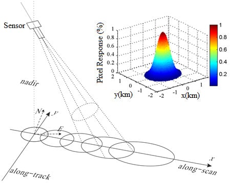
3. Simulation of the 500-m/1-km Albedo PSF Model

3.1. Method

The objective of the modeling is to depict the ground area that contributes to the response of each 1-km albedo pixel and estimate the relative response distribution function f_A, which is defined as the PSF model of each albedo pixel. The ground area is denoted as the support of the PSF model.

The geographic coordinates of each pixel in the MCD43 or GLASS02 albedo images were fixed according to the SIN grid, and the values of the pixel for both products were derived from the relevant MODIS reflectance data. Therefore, a position-oriented simulation method was adapted in this study to simulate the PSF model of each albedo pixel. The method involves searching all ungridded positions of the relevant reflectance observation cells and identifying the contributions of each observation to the albedo PSF in a united coordinate system in which the origin is at the albedo pixel center. The simulation of the albedo PSF model comprises two stages.

The first stage involves describing the SRCs of the relevant ungridded MODIS observations. The PSF of an ungridded MODIS observation cell exhibits triangular shapes in the track direction and rectangular shapes in the scan direction (referred to as the “triangular model”) under laboratory conditions (Equation (1)) [1]. The reflected radiation from the ground surface is affected by the atmosphere prior to being received by the on-orbit sensors. A Gaussian function can be used to simulate the effect of the atmosphere on the PSF (Equation (2)) [25]. Thus, the actual spatial response model of the MODIS reflectance data is the convolution of the triangular model with the Gaussian model (Equation (3), Figure 3).

$$f_{triangular}(x\text{,}y)=\{\begin{array}{cc}1-\frac{\left|x-x_0\right|}{M}\hfill & \left|x-x_{\text{0}}\right|\le M\cap \left|y-y_{\text{0}}\right|\le N\\ 0& \text{otherwise}\end{array}$$

(1)

$$f_{Gaussian}(x\text{,}y)=exp(-\frac{{(x-x_{\text{0}})}^2+{(y-y_{\text{0}})}^2}{2{\text{σ}}^2})$$

(2)

$$f_{ref\_Actual}(x\text{,}y)=f_{Gaussian}(x\text{,}y)\times f_{triangular}(x\text{,}y)$$

(3)

where, x and y refer to the scan-direction coordinates and track-direction coordinates, respectively, which originated at the center point (x₀, y₀) within the support of the PSF. σ denotes the standard deviation of the Gaussian function; it is given the value of 50 m [11]. M and N, which consist of half the size of the support, refer to the scan direction and track direction, respectively. These symbols are also utilized in Section 4.

Although the albedo at each grid cell is calculated from a series of gridded L2G-lite daily reflectance data, all of the ground area covered by the GIFOV of the relevant ungridded reflectance observations contributes to the albedo value. The cell positions and view geometry information can be extracted from the ungridded MOD/MYD03 (Level 1, Collection 005) data, including the pixel center coordinates, view zenith angle, view azimuth angle, and scan angle between the scan direction and west-east direction. The PSF model of each reflectance pixel is deformed in the albedo inversion process. The deformation direction is identified by the scan angle, and the deformation degree is determined by the view zenith angle (Figure 4). The PSF of albedo pixels is discussed in Universal Transverse Mercator (UTM) coordinate system because this system preserves angles and approximates shapes. x points in the east direction, and y points in the north direction. Therefore, the reflectance PSF must be rotated and transformed before the albedo PSF simulation.

Figure 3. Simulation of the PSF of the MODIS reflectance data.

Figure 3. Simulation of the PSF of the MODIS reflectance data.

Figure 4. Illustration of the PSF transformation of a reflectance pixel [11].

Figure 4. Illustration of the PSF transformation of a reflectance pixel [11].

The deformed PSF model of each observation cell was simulated in four steps:

(1) Establish the reflectance PSF model F₀ on the sensor’s focal plane (Equation (3), Figure 3).

(2) Project the model to the ground surface according to the VZA θ_v. The radiance received by a sensor within one pixel is regarded as parallel light because the width of the GIFOV is significantly smaller than the distance between the sensor and Earth. F_g, the projection of F₀ on the tangent plane at the center of the observation on the ground surface, is obtained by stretching F₀ along the scan direction using the VZA (Equation (4)), as the VZA is measured with respect to the local ellipsoid normal [26]. Because Earth’s curvature effects are small over the area of a single pixel, these effects are reasonably ignored in the calculation of the observation area [1,26].

$$\begin{array}{l}{F}_g(x_g,y_g)=F_0(x_0,y_0)\\ {(x_g,y_g)}^T=\left[\begin{array}{cc}{(\cos {\theta }_v)}^{-1}& 0\\ 0& 1\end{array}\right]{(x_0,y_0)}^T\end{array}$$

(4)

where x₀ and y₀ are the coordinates on the sensor’s focal plane and x_g and y_g are the coordinates on the ground surface plane. x of both the coordinate systems is along the scan direction.

(3) Rotate F_g according to the sensor azimuth angle a_s, which is relative to local geodetic north [26], to obtain F_gs and ensure that the x direction is east (Equation (5)).

$$\begin{array}{l}{F}_{gs}(x_{gs},y_{gs})=F_g(x_g,y_g)\\ {(x_{gs},y_{gs})}^T=\left[\begin{array}{cc}\cos a_s& -\sin a_s\\ \sin a_s& \cos a_s\end{array}\right]{(x_g,y_g)}^T\end{array}$$

(5)

where x_gs and y_gs are the coordinates rotated from x_g and y_g, respectively.

(4) Move F_gs on the plane to align its center with the albedo pixel center to obtain F_gsc (Equation (6)).

$$\begin{array}{l}{F}_{gsc}(x_{gsc},y_{gsc})=F_{gs}(x_{gs},y_{gs})\\ {(x_{gsc},y_{gsc},1)}^T=\left[\begin{array}{ccc}1& 0& \Delta x\\ 0& 1& \Delta y\\ 0& 0& 1\end{array}\right]{(x_{gs},y_{gs},1)}^T\end{array}$$

(6)

where x_gsc and y_gsc are the coordinates with an origin at the albedo pixel center and ∆x and ∆y corresponds to the offset between the origin of F_gs and the albedo pixel center.

The second stage involves deriving the albedo PSF model (f_A) from the transformed PSF of each reflectance observation cell (F_gscⁱ). f_A is defined for each 1-km albedo pixel, whose origin is at the grid center of the pixel. However, considering that the PSF model of the albedo is influenced by several complicated factors, including the gridding process, multiple resampling under random weather conditions and a nonlinear algorithm, the simulation of the albedo PSF was simplified; in particular, the contribution of each reflectance observation cell was linearly accumulated and averaged.

The L2G-lite daily MOD/MYD09 product is derived from a gridding process that composites different orbits of geometrically corrected satellite observations. The compositing routine of the Collection 005 MODIS albedo product calculates the weighted sum of all co-area observations according to their obscov, which means that all relevant observations from different orbits contribute to the PSF response of the reflectance grid and thus the albedo grid. Therefore, the set of PSF estimations from all orbits (typically 1 orbit per day, occasionally 2 or 3 orbits) were collected and averaged to approximate f_A. The simulation time period employed was one year (365 days, from the first day of the year), instead of the 16-day period, to reduce the variability caused by the limited amount of available reflectance images in deriving the albedo for a 16-day period, to overcome the influence caused by cloud and data gaps and to determine the common characteristics of the albedo image spatial responses.

The coefficients of f_A were fitted from the accumulated reflectance PSF of the entire year. f_A was normalized to set the maximum value of the albedo spatial response to 1. Therefore, the integral of the f_A over its support must be divided while using f_A as the upscaling weight matrix of albedo.

For the MCD43A3 albedo, the simulation was performed at a 500-m scale; then, the 2 × 2 neighboring pixels were aggregated to form the 1-km MCD43B3 pixel PSF distribution. For the GLASS02 albedo, the simulation was directly conducted at a 1-km scale.

3.2. Result

The PSF of 300 evenly distributed 500-m MCD43A3 albedo pixels was simulated over the midstream area using 365-day Terra-MODIS reflectance data. Because the simulated PSF of each pixel exhibits similar characteristics, the average result is demonstrated in Figure 5.

Figure 5. The average of the simulated albedo response (f_A) was solely derived from the viewing zenith angle and the viewing azimuth angle available in the MOD03 (Terra) and MYD03 (Aqua) products over 365 days and 300 pixels. (a) Simulated 500-m albedo response (f_A) for MOD43A3. (b) Simulated 500-m albedo response (f_A) for MYD43A3. (c) Simulated 500-m albedo response (f_A) for MCD43A3.

Figure 5. The average of the simulated albedo response (f_A) was solely derived from the viewing zenith angle and the viewing azimuth angle available in the MOD03 (Terra) and MYD03 (Aqua) products over 365 days and 300 pixels. (a) Simulated 500-m albedo response (f_A) for MOD43A3. (b) Simulated 500-m albedo response (f_A) for MYD43A3. (c) Simulated 500-m albedo response (f_A) for MCD43A3.

The elliptical Gaussian function is used to mathematically describe the simulated PSF of albedo pixels, the function is expressed in Equation (7).

$$\begin{array}{l}{f}_{Gaussian}(x\text{,}y)=exp(-\frac{x{\prime }^{\text{2}}+c^{\text{2}}y{\prime }^{\text{2}}}{2s^{\text{2}}})\\ x\prime =(x-x_0)\cos \theta +(y-y_0)\sin \theta \\ y\prime =-(x-x_0)\sin \theta +(y-y_0)\cos \theta \end{array}$$

(7)

where c is the ratio between the semi-major and semi-minor axes of the projected ellipse, s is the standard deviation of the elliptical Gaussian function, and θ denotes the rotation angle of the ellipse from the east bearing (counterclockwise is positive).

Function 11 was used to fit the simulated albedo response of each pixel (the average is shown in Figure 5). The support of the albedo LSF was wider than its nominal resolution due to the proximate contributions of the imaging system and the non-overlapping GIFOVs of the multi-angle reflectance data used to derive the albedo.

The coefficients of the function were calculated using the least squares error criteria. Then, the mean coefficients derived from the 300 pixels distributed in the midstream area were calculated (row 2 of Table 2). Considering the latitudinal difference between midstream and downstream of the Heihe River Basin, 300 additional randomly distributed pixels downstream were analyzed according to the abovementioned procedures; the average coefficients are listed in row 3 of Table 2.

Table 2. Average coefficients (with the unbiased standard deviation) of 300 pixels in the middle and lower reaches of the Heihe River Basin.

Scope	Sensor	Product	c	s (m)	θ (°)	RMSE
midstream	Terra	MOD43A3	1.43 (0.053)	368.69 (10.62)	−23.28 (2.45)	0.059 (0.0045)
downstream	Terra	MOD43A3	1.45 (0.047)	376.90 (7.54)	−23.89 (2.17)	0.056 (0.0041)
Average *	Aqua	MYD43A3	1.4181 (0.0748)	390.76 (12.93)	22.2688 (3.52)	0.0628 (0.0056)
Average	Terra + Aqua	MCD43A3	1.1831 (0.0514)	375.0916 (25.82)	1.9209 (8.4298)	0.0568 (0.0087)

* Average corresponds to the average coefficients midstream and downstream.

Table 2. Average coefficients (with the unbiased standard deviation) of 300 pixels in the middle and lower reaches of the Heihe River Basin.

Scope	Sensor	Product	c	s (m)	θ (°)	RMSE
midstream	Terra	MOD43A3	1.43 (0.053)	368.69 (10.62)	−23.28 (2.45)	0.059 (0.0045)
downstream	Terra	MOD43A3	1.45 (0.047)	376.90 (7.54)	−23.89 (2.17)	0.056 (0.0041)
Average *	Aqua	MYD43A3	1.4181 (0.0748)	390.76 (12.93)	22.2688 (3.52)	0.0628 (0.0056)
Average	Terra + Aqua	MCD43A3	1.1831 (0.0514)	375.0916 (25.82)	1.9209 (8.4298)	0.0568 (0.0087)

* Average corresponds to the average coefficients midstream and downstream.

The comparison between these two groups of parameters indicates that the simulated responses of the pixels in the midstream and downstream areas are similar, which supports the notion that the same function is approximately acceptable in the entire Heihe River Basin. However, a small difference exists between the coefficients of the two areas, which may be ascribed to the different latitudes because the scan-direction resolution of the MODIS reflectance data is dependent on the latitude [3].

This discussion focuses on the MOD43A3 albedo response, which is solely derived from Terra-MODIS MOD03 data. For the MYD43B3 albedo, which is inverted from Aqua-MODIS data, the PSF model is symmetric about the east bearing (row 3 of Table 2) because MODIS is on a descending orbit for Terra or an ascending orbit for Aqua. The commonly used MCD43A3 albedo employs the Terra-MODIS and the Aqua-MODIS reflectance data as source data; thus, the parameter θ of the PSF model is approximately 0° (row 4 of Table 2). The combination of Terra and Aqua enhances the fluctuation of θ and s, which correspond to the orientation and the standard deviation of the elliptical Gaussian model, respectively. The parameter c of MCD43A3 is closer to 1 compared to those of MOD43A3 and MYD43A3; thus, the projection of the PSF model resembles a circle.

4. Discussion

4.1. Comparison of the Simulated Albedo PSF Model with Other PSF Models

The PSF model can be employed as the spatial weight distribution function in albedo upscaling, by weighted aggregation of the 30-m albedo into the 1-km albedo. The efficiency of different PSF models is reflected in the comparison between the upscaled albedo images and the coarse-resolution albedo images, particularly in heterogeneous regions in which neighboring areas exhibit strong contrasts [11]. One concern is that the comparison results are also influenced by many other factors, particularly the geolocation error and the scale effect [22]. We employed a least-squares sub-pixel geometric matching method to search and compensate for the geolocation error and selected a flat experimental area without influential terrain to prevent the scale effect. To compare the different parametric PSF models (e.g., Gaussian model [17] or Gaussian-like model [18] and the simulated model in this study), we computed the determination coefficient r² as the goodness of fit between the 1-km albedo images upscaled from the 30 m albedo and the 1-km albedo products (refer to MCD43B3 and GLASS02, respectively, in this paper); r² is not influenced by the bias between the images.

Five commonly used PSF models were selected as the reference models (Figure 6). These models were employed as the convolution kernels to aggregate the 30-m HJ albedo to the 1-km scale. The models were normalized by their total response within the convolution window in use. The upscaled 1-km albedo is expressed as Equation (8),

$$A_{c,l}=\frac{{\displaystyle {\mathrm{\int }}_{(x\text{,}y)\in D}{f}_{PSF}(x\text{,}y)\alpha (x\text{,}y)}}{{\displaystyle {\mathrm{\int }}_{(x\text{,}y)\in D}{f}_{PSF}(x\text{,}y)}}$$

(8)

where A_c,l denotes the simulated 1-km albedo; c and l refer to the pixel column and row number, respectively, in the 1-km albedo image; D is the corresponding pixel set in the HJ albedo image, which is dependent on the size of the PSF; f is the PSF model; α represents the HJ albedo value; and for albedo pixels, x and y refer to the east-direction coordinates and north-direction coordinates, respectively, of each HJ pixel in the image coordinate system that is centered on the 1-km pixel center.

The mathematical expressions of the five predicted PSF models are provided in this section.

(1) The rectangular PSF model assumes that the weight is uniformly distributed over a rectangle (Equation (9)):

$$f_{PSF\_Rectangular}(x\text{,}y)=\{\begin{array}{ll}1& \left|x-x_{\text{0}}\right|\le M\cap \left|y-y_{\text{0}}\right|\le N\\ 0& \text{otherwise}\end{array}$$

(9)

(2) The Gaussian distribution (Equation (10)) is considered to be consistent with more realistic situations and fits the MODIS reflectance data [10]:

$$f_{PSF\_Gaussian}(x\text{,}y)=exp(-\frac{{(x-x_{\text{0}})}^2+{(y-y_{\text{0}})}^2}{2{\text{σ}}^2})$$

(10)

where σ denotes the standard deviation of the Gaussian function, which determines the amplitude of the distribution ($0.4\sqrt{M\times N}$ in the study).

(3) The triangular model was employed because it is the raw MODIS PSF model, i.e., the PSF of MODIS detectors [1], which is described in Equation (11):

$$f_{PSF\_Triangular}(x\text{,}y)=\{\begin{array}{cc}1-\frac{\left|x-x_0\right|}{M}\hfill & \left|x-x_{\text{0}}\right|\le M\cap \left|y-y_{\text{0}}\right|\le N\hfill \\ 0& \text{otherwise}\end{array}$$

(11)

(4) The cosine model is defined as Equation (12):

$$f_{PSF\_Cosine}(x\text{,}y)=cos(\sqrt{\frac{{(x-x_{\text{0}})}^{\text{2}}+{(y-y_{\text{0}})}^{\text{2}}}{M^2+N^2}}\times \frac{\pi }{4})$$

(12)

(5) The circular model is formulated as Equation (13):

$$f_{PSF\_Circular}(x\text{,}y)=\{\begin{array}{ll}1& {(x-x_{\text{0}})}^{\text{2}}+{(y-y_{\text{0}})}^{\text{2}}<M^2+N^2\\ 0& \text{otherwise}\end{array}$$

(13)

PSFs have two main features, namely, shape and size, which describe the SRCs of remote sensing images. The model function type determines the PSF shape. The PSF size was described using two indicators by considering the difference between the uniform and non-uniform response models. Here the uniform means that the response is constant within the PSF support, which correspond to models 1 and 5, thus the other three models are non-uniform. The first approach uses the convolution window size to define the PSF size in two dimensions (which corresponds to the support sizes M and N defined in Section 3), which delimits the 30-m pixels that were utilized for a 500-m pixel. The second approach defines the parameter Rσ, which is expressed in Equation (14),

$$R\text{σ=}\sqrt{\frac{{\displaystyle \sum \left(\left({(x-x_{\text{0}})}^{\text{2}}+{(y-y_{\text{0}})}^{\text{2}}\right)\cdot f_{PSF}\right)}}{{\displaystyle \sum f_{PSF}}}},\left|x-x_{\text{0}}\right|\le M\cap \left|y-y_{\text{0}}\right|\le N$$

(14)

where (x − x₀)² + (y − y₀)² corresponds to the distance between the 30-m pixel to the origin (the 1-km pixel center), and f_PSF is the PSF model value used as a weight. The sums are defined over the entire support for uniform models, whereas they are defined over the positions that contribute to 95% of the PSF for non-uniform models. Compared with the convolution window size or the remaining two-dimensional PSF size indicators, such as the full width at half maximum (FWHM), which has been applied to describe the Gaussian model size [3,18], Rσ integrates the two-dimensional PSF size into one value while considering the response distribution. Rσ is a standardized PSF size indicator that is comparable among uniform and non-uniform models because it can reflect the smaller contribution of the peripheral pixels. Using the Gaussian model as an example, every 30-m pixel around the 500-m pixel theoretically has a non-zero weight, i.e., the convolution window size can be arbitrarily large. However, the contributions of the pixels beyond 95% can be disregarded in practice, and the pixels that work are delimited by Rσ.

Figure 6. Five reference PSF models: (a) Rectangular; (b) Cosine; (c) Triangular; (d) Gaussian; and (e) Circular.

Figure 6. Five reference PSF models: (a) Rectangular; (b) Cosine; (c) Triangular; (d) Gaussian; and (e) Circular.

The fitting precision of different models can only be compared by the same Rσ. To describe the explicit relationship between Rσ and the FWHM, Figure 7 illustrates the correspondence of Rσ with the FWHM for a rectangular model and a Gaussian model. Because the PSF value of a rectangular model only varies in one direction, the corresponding FWHM in that direction was set as the x-axis in Figure 7. The Gaussian PSF model is isotropic; thus, the FWHM of the major axis (FWHM_a) and the FWHM of the minor axis (FWHM_b) are equivalent. The Rσ of the simulated elliptical Gaussian model for MCD43A3 in the Heihe River Basin is 491 m, whereas the FWHM_a and FWHM_b are 883 and 747 m, respectively.

Figure 7. Comparison of the FWHMs for the rectangular model and Gaussian model.

Figure 7. Comparison of the FWHMs for the rectangular model and Gaussian model.

The inherent errors in assigning geolocation coordinates to albedo observations may cause noise in the analysis, or “geolocation errors” [27]. For example, the geolocation errors of MODIS L1B data are less than 50 m at 1 sigma and the nadir [4,12]. Thus, the geolocation errors were considered in the simulation, as identified via a least-squares sub-pixel geometric matching method. This method determines the optimum offset using the grayscale gradient of the HJ albedo image and the maximum correlation between the simulated albedo and the albedo product at a 1-km resolution [28]. The geolocation offset was compensated for prior to the simulation.

4.2. Application of the Models in Albedo Upscaling at 500-m

The reference models with various Rσ were employed to upscale the 30-m HJ albedo to 500 m with the simulated elliptical Gaussian model. The simulated albedos from the PSF models with increasing Rσ were compared with the MCD43A3 albedos. The r² between the simulated albedo and the albedo products was used to evaluate the goodness of fit. Higher r² values indicate a better fit of the PSF model shape and size for the albedo product.

Figure 8 shows the comparison between the 500-m upscaled albedo and the MCD43A3 albedo midstream and downstream of the Heihe River Basin. The following conclusions are noted:

(1) Comparing the r² of the simulated model (the elliptical Gaussian model described in Section 3) and other reference models at the same Rσ, the simulated model can maintain a slight higher r² midstream and downstream for the majority of the datasets. The r² of the Gaussian model is similar or equal to the r² of the simulated model for m1, m2, m3, m8 and d1 because the shape of the Gaussian model is similar to the elliptical Gaussian model. The only difference is that the latter model can reflect the different LSFs in the x and y directions as well. This demonstrates the feasibility of using the Gaussian model as a substitute when the precise parameters of the elliptical Gaussian model cannot be determined.

(2) Using a uniform rectangular model of 500-m × 500-m convolution window is equivalent to directly aggregating the 30-m albedo into 500-m scale albedo without considering the PSF effect. The Rσ of the 500-m uniform rectangular model is approximately 200 m and is significantly smaller than the Rσ of the simulated model, which corresponds to a lower r² between the upscaled albedo and the 500-m albedo product than the simulated model in all cases illustrated in Figure 8. This finding proves that take the PSF effect must be considered in albedo upscaling. The discrepancy of r² is approximately 0.03–0.05 midstream and is approximately 0.015–0.04 downstream because the surface heterogeneity is slightly stronger midstream.

(3) The Gaussian and triangular models exhibit higher r² values than other reference models; this finding confirms that the response distribution within the 500-m MCD43A3 pixel is non-uniform. The r² of different models for the same Rσ does not vary as much as the r² with an increased Rσ, demonstrating that the PSF size has a greater impact on the upscaling accuracy than the PSF shape.

(4) According to the sub-pixel registration prior to the albedo upscaling, the geographic coordinates of the MCD43A3 albedo in this study have a random geolocation error that is less than half of a pixel size and shifts to the northwest (Figure 9).

Figure 8. Variation in r² (between the upscaled 500-m albedo and the MCD43A3 albedo) and Rσ. Each plot corresponds to a dataset in Table 1. (a) No. m1 (30 June 2012; the midstream); (b) No. m2 (3 August 2012; the midstream); (c) No. m3 (2 September 2012; the midstream); (d) No. m5 (8 March 2013; the midstream); (e) No. m6 (2 April 2013; the midstream); (f) No. m7 (2 May 2013; the midstream); (g) No. m8 (11 June 2013; the midstream); (h) No. d1 (2 April 2013; the downstream); (i) No. d2 (9 May 2013; the downstream); (k) No. d3 (2 August 2013; the downstream); (l) No. d4 (4 September 2013; the downstream); and (m) No.: d5 (3 October 2013; the downstream).

Figure 8. Variation in r² (between the upscaled 500-m albedo and the MCD43A3 albedo) and Rσ. Each plot corresponds to a dataset in Table 1. (a) No. m1 (30 June 2012; the midstream); (b) No. m2 (3 August 2012; the midstream); (c) No. m3 (2 September 2012; the midstream); (d) No. m5 (8 March 2013; the midstream); (e) No. m6 (2 April 2013; the midstream); (f) No. m7 (2 May 2013; the midstream); (g) No. m8 (11 June 2013; the midstream); (h) No. d1 (2 April 2013; the downstream); (i) No. d2 (9 May 2013; the downstream); (k) No. d3 (2 August 2013; the downstream); (l) No. d4 (4 September 2013; the downstream); and (m) No.: d5 (3 October 2013; the downstream).

Figure 9. Average geometric offset of the MCD43A3 image of each dataset. “Set No.” refers to Table 1 (x is eastward and y is northward).

Figure 9. Average geometric offset of the MCD43A3 image of each dataset. “Set No.” refers to Table 1 (x is eastward and y is northward).

4.3. Comparison of the PSFs of MCD43B3 and GLASS02 at the 1-km Scale

In this study, PSF simulations were also conducted at the 1-km scale for the MCD43B3 and GLASS02 albedo products, as discussed in Section 3.1. The PSF of MCD43B3 can be simulated by averaging the PSF of the corresponding 2 × 2 neighboring 500-m MCD43A3 pixels. The simulated model of MCD43A3 (discussed in Section 3.2) shows greater support than its ground sample distance (GSD), which is supported in Section 4.2 by a comparison among PSF models with various Rσ values. Therefore, the average PSF model of 2 × 2 neighboring MCD43A3 pixels remains similar to the elliptical Gaussian model. The obtained albedo response distribution was fitted using Equation (7) (Table 2).

The PSF model of the GLASS02 albedo product can be simulated using the simulation method introduced in Section 3.1 at the 1-km scale because the GLASS02 albedo product was directly calculated from daily 1-km MODIS reflectance products with a smooth filtering process using 17-day albedo products. The obtained albedo response distribution was fitted using Equation (7) (Table 3). The comparison of the simulated Rσ and FWHM of MCD43B3 and GLASS02 indicates a smaller spatial response support of a MCD43B3 pixel (Figure 10).

Table 3. Average geometric offset of the 1-km MCD43B3 albedo and the GLASS02 albedo (x is eastward and y is northward).

Product	c	s (m)	θ (°)	Rσ (m)	FWHMa (m)	FWHMb (m)
MCD43B3	1.6	482.09	−26.17	568.4	1135	709
GLASS02	1.36	700	2.3	868.86	1648	1212

Table 3. Average geometric offset of the 1-km MCD43B3 albedo and the GLASS02 albedo (x is eastward and y is northward).

Product	c	s (m)	θ (°)	Rσ (m)	FWHMa (m)	FWHMb (m)
MCD43B3	1.6	482.09	−26.17	568.4	1135	709
GLASS02	1.36	700	2.3	868.86	1648	1212

Figure 10. Illustration of the pixel response of two typical 1-km albedo products. (a) MCD43B3; (b) GLASS02.

Figure 10. Illustration of the pixel response of two typical 1-km albedo products. (a) MCD43B3; (b) GLASS02.

The five reference models with various Rσ were used to aggregate the 1-km resolution albedo using the 30-m HJ albedo data. The r² between the upscaled albedo and the 1-km albedo products for four datasets (introduced in Table 1) were calculated. The variation in the average correlation coefficients of the four datasets with Rσ are shown in Figure 11; and the corresponding geolocation shift of the MCD43B3 and GLASS02 albedos is listed in Table 4.

Figure 11 demonstrates the effect of the PSF on the albedo upscaling accuracy at the 1-km scale.

Figure 11. Variation in the correlation coefficients between the 1-km albedo products and the upscaled value with Rσ. (a) MCD43B3; (b) GLASS02.

Figure 11. Variation in the correlation coefficients between the 1-km albedo products and the upscaled value with Rσ. (a) MCD43B3; (b) GLASS02.

First, the variation trend of r² with Rσ is different for MCD43B3 and GLASS02. The optimal Rσ of MCD43B3 is smaller than the optimal Rσ of GLASS02, which reveals the smaller PSF size of MCD43B3 and a stronger adjacency effect on GLASS02. This finding is consistent with the previous comparison results for the parameters of the simulated model, which demonstrate the impact of the two inversion methods on the PSF model of the derived albedo products.

Second, for the reference PSF model shown in Figure 11, the r² values peak at nearly the same Rσ, which is approximately 700 m for the MCD43 product and 1050 m for the GLASS02 product. The Rσ of the 1-km rectangular model (equivalent to direct aggregation without considering the PSF effect) is 380 m. The corresponding r² of both products is apparently lower than the r² using the simulated model or other models at the optimal Rσ. Compared with the 1-km rectangular model, the improvement in the r² for MCD43B3 using the simulated PSF model is 3.07% and 9.40% for GLASS02.

A comparison of the reference models reveals several similarities to the 500-m scale comparison. (1) The elliptical Gaussian model has a slightly higher r² compared with other reference models at the same Rσ. However, the Rσ of the simulated model does not reach the optimal Rσ of each product in the area due to the imprecise simulation of the nonlinearity in the transformation from the reflectance PSF to the albedo PSF. (2) The Gaussian model is a better choice for depicting the albedo PSF compared with other reference models. Because the highest r² of the different models are nearly identical, the PSF size (expressed by Rσ) dominates the upscaling accuracy instead of the PSF shape, that is, the adjacency effect exhibits a larger influence on the upscaling accuracy than the distribution of the spatial response. (3) The sub-pixel geolocation error in both 1-km albedo products exhibits some stochastic behavior below 0.5 pixels (Table 4) due to the inherent geometric registration errors in the reflectance data, and it is further distorted by the resampling and reprojection conversion during the inversion.

Table 4. Average geometric offset of the 1-km MCD43B3 albedo and the GLASS02 albedo (x is eastward and y is northward).

HJ Date	MCD43		GLASS02
	x	y	x	y
20120630	−69	100	−104	−18
20120803	−102	62	−231	−121
20120902	−187	101	−202	−121
20120930	−119	168	−272	−98

Table 4. Average geometric offset of the 1-km MCD43B3 albedo and the GLASS02 albedo (x is eastward and y is northward).

HJ Date	MCD43		GLASS02
	x	y	x	y
20120630	−69	100	−104	−18
20120803	−102	62	−231	−121
20120902	−187	101	−202	−121
20120930	−119	168	−272	−98

5. Conclusions

The main objective of this study is to model the spatial responses of coarse-resolution albedo products derived from MODIS data, which is an important issue for many studies, such as the validation of remote sensing products and multi-scale data fusion. We have simulated the PSF model to describe the SRCs of two series of commonly used coarse-resolution albedo products derived from MODIS reflectance data over the Heihe River Basin in northwest China. Two complementary steps are included in the analysis: the simulation based on the PSF of the observation cells and the application of the simulated model in albedo upscaling with cross-validation using other reference models. The simulation results and comparison using various reference models are highly consistent; thus, the anisotropy of the spatial response in albedo upscaling must be considered.

The simulation of the 500-m/1-km albedo PSF was dependent on two assumptions. First, the PSF of the MODIS swath data was adopted as the original information on the albedo spatial response characteristics. This simplification does not consider the impact of the gridding process on the reflectance data aligned with the SIN grid pixels. Thus, the magnitude of the PSFs due to the gridding process was slightly underestimated in the model, as demonstrated by the cross-validation using the reference models, i.e., the Rσ of the simulated model is smaller than the optimal Rσ. Second, the PSF simulation was conducted in a UTM projection system. The PSF size described using UTM coordinates is closer to the distance on the curved surface, but slightly different than that under sinusoidal projection.

The simulation provides a feasible spatial response model (the simulated elliptical Gaussian model) for the target coarse-resolution albedo products over the Heihe River Basin with substitute models. How do our results apply to areas outside of the Heihe River Basin? The albedo PSF can change with position for two reasons: first, the deformation of MODIS reflectance pixels is aligned with the SIN grid rows and columns. Campagnolo et al. [3] examined the variation in the estimated FWHM of the MODIS L2G product for both the row and column directions. To connect our results for the PSF size with this finding, the relationships between Rσ and the FWHM of non-uniform models were determined (Figure 7). However, the relevance is not straightforward because the PSF model of the albedo product is also influenced by the multi-day data quality and resampling, with the exception of the PSF of the observation cells. Thus, this question posed should be addressed in future studies to assess the variation in the albedo PSF with position. The proposed methods can also be applied to modeling the spatial response characteristics of other high-order MODIS products.

References

1. Tan, B.; Woodcock, C.E.; Hu, J.; Zhang, P.; Ozdoganb, M.; Huang, D.; Yang, W.; Knyazikhina, Y.; Myneni, R.B. The impact of gridding artifacts on the local spatial properties of MODIS data: Implications for validation, compositing, and band-to-band registration across resolutions. Remote Sens. Environ. 2006, 105, 98–114. [Google Scholar] [CrossRef]
2. Barnes, W.L.; Pagano, T.S.; Salomonson, V.V. Prelaunch characteristics of the moderate resolution imaging spectroradiometer (MODIS) on EOS-AM1. IEEE Trans. Geosci. Remote Sens. 1998, 36, 1088–1100. [Google Scholar] [CrossRef]
3. Campagnolo, M.L.; Montano, E.L. Estimation of effective resolution for daily MODIS gridded surface reflectance products. IEEE Trans. Geosci. Remote Sens. 2014, 52, 5622–5632. [Google Scholar] [CrossRef]
4. Wolfe, R.E.; Nishihama, M.; Fleig, A.J.; Kuyper, J.A.; Roy, D.P.; Storey, J.C.; Patt, F.S. Achieving sub-pixel geolocation accuracy in support of MODIS land science. Remote Sens. Environ. 2002, 83, 31–49. [Google Scholar] [CrossRef]
5. Justice, C.O.; Vermote, E.; Townshend, J.R.; Defries, R.; Roy, D.P.; Hall, D.K.; Salomonson, V.V.; Privette, J.L.; Riggs, G.; Strahler, A. The moderate resolution imaging spectroradiometer (MODIS): Land remote sensing for global change research. IEEE Trans. Geosci. Remote Sens. 1998, 36, 1228–1249. [Google Scholar] [CrossRef]
6. Townshend, J.R.G.; Huang, C.; Kalluri, S.N.V.; Defries, R.S.; Liang, S.; Yang, K. Beware of per-pixel characterization of land cover. Int. J. Remote Sens. 2000, 21, 839–843. [Google Scholar] [CrossRef]
7. Du, H.; Voss, K.J. Effects of point-spread function on calibration and radiometric accuracy of ccd camera. Appl. Opt. 2004, 43, 665–670. [Google Scholar] [CrossRef] [PubMed]
8. Bitlis, B.; Jansson, P.A.; Allebach, J.P. Parametric point spread function modeling and reduction of stray light effects in digital still cameras. Proc. SPIE 2007. [Google Scholar] [CrossRef]
9. Zhao, C.; Qi, B.; Youn, E.; Yin, G.; Nansen, C. Use of neighborhood unhomogeneity to detect the edge of hyperspectral spatial stray light region. Optik-Int. J. Light Electron Opt. 2014, 125, 3009–3012. [Google Scholar] [CrossRef]
10. Barker, J.L.; Markham, B.L.; Burelbach, J.W. MODIS Image Simulation from Landsat TM Imagery; Global Change and Education ASPRS/ACSM/RT 92; American Society for Photogrammetry and Remote Sensing: Washington, DC, USA, 1992. [Google Scholar]
11. Duveiller, G.; Baret, F.; Defourny, P. Crop specific green area index retrieval from MODIS data at regional scale by controlling pixel-target adequacy. Remote Sens. Environ. 2011, 115, 2686–2701. [Google Scholar] [CrossRef]
12. Huang, C.; Townshend, J.R.G.; Liang, S.; Kalluri, S.N.V.; DeFries, R.S. Impact of sensor’s point spread function on land cover characterization: Assessment and deconvolution. Remote Sens. Environ. 2002, 80, 203–212. [Google Scholar] [CrossRef]
13. Zong, Y.; Brown, S.W.; Meister, G.; Barnes, R.A.; Lykke, K.R. Characterization and Correction of Stray Light in Optical Instruments. Proc. SPIE 2007. [Google Scholar] [CrossRef]
14. Pilz, M.; Honold, S.; Kienle, A. Determination of the optical properties of turbid media by measurements of the spatially resolved reflectance considering the point-spread function of the camera system. J. Biomed. Opt. 2008, 13, 4047–4053. [Google Scholar] [CrossRef] [PubMed]
15. Hayes, D.J.; Cohen, W.B. Spatial, spectral and temporal patterns of tropical forest cover change as observed with multiple scales of optical satellite data. Remote Sens. Environ. 2007, 106, 1–16. [Google Scholar] [CrossRef]
16. Busetto, L.; Meroni, M.; Colombo, R. Combining medium and coarse spatial resolution satellite data to improve the estimation of sub-pixel NDVI time series. Remote Sens. Environ. 2008, 112, 118–131. [Google Scholar] [CrossRef]
17. Susaki, J.; Yasuoka, Y.; Kajiwara, K.; Honda, Y.; Hara, K. Validation of MODIS albedo products of paddy fields in Japan. IEEE Trans. Geosci. Remote Sens. 2007, 45, 206–217. [Google Scholar] [CrossRef]
18. Mira, M.; Courault, D.; Olioso, A.; Weiss, M.; Marloie, O.; Baret, F.; Hagolle, O.; Gallego-Elvira, B. Validation of MODIS albedo products with high resolution albedo estimates from FORMOSAT-2. In Proceedings of the 2013 IEEE International Geoscience and Remote Sensing Symposium (IGARSS), Melbourne, VIC, Australia, 21–26 July 2013; pp. 3250–3253.
19. Schaaf, C.B.; Gao, F.; Strahler, A.H.; Lucht, W.; Li, X.; Tsang, T.; Strugnell, N.C.; Zhang, X.; Jin, Y.; Muller, J.-P. First operational BRDF, albedo nadir reflectance products from MODIS. Remote Sens. Environ. 2002, 83, 135–148. [Google Scholar] [CrossRef]
20. Liu, N.; Liu, Q.; Wang, L.; Liang, S.; Wen, J.; Qu, Y.; Liu, S. Mapping spatially-temporally continuous shortwave albedo for global land surface from MODIS data. Hydrol. Earth Syst. Sci. Discuss. 2012, 9, 9043–9064. [Google Scholar] [CrossRef]
21. Qu, Y.; Liu, Q.; Liang, S.; Wang, L.; Liu, N.; Liu, S. Direct-estimation algorithm for mapping daily land-surface broadband albedo from MODIS data. IEEE Trans. Geosci. Remote Sens. 2014, 52, 907–919. [Google Scholar] [CrossRef]
22. Peng, J.; Liu, Q.; Wen, J.; Liu, Q.; Tang, Y.; Wang, L.; Dou, B.; You, D.; Sun, C.; Zhao, X. Multi-scale validation strategy for satellite albedo products and its uncertainty analysis. Sci. China Earth Sci. 2015, 58, 573–588. [Google Scholar] [CrossRef]
23. Li, X.; Cheng, G.; Liu, S.; Xiao, Q.; Ma, M.; Jin, R.; Che, T.; Liu, Q.; Wang, W.; Qi, Y. Heihe watershed allied telemetry experimental research (HiWATER): Scientific objectives and experimental design. Bull. Am. Meteorol. Soc. 2013, 94, 1145–1160. [Google Scholar] [CrossRef]
24. Zhong, B.; Nie, A.; Yang, A.; Zhang, H.; Ma, P.; Liu, Q. HiWATER: Land Cover Map of Heihe River Basin; Heihe Plan Science Data Center: Lanzhou, China, 2014. [Google Scholar] [CrossRef]
25. Ojansivu, V.; Heikkilä, J. Blur insensitive texture classification using local phase quantization. In Image and Signal Processing; Springer: Berlin/Heidelberg, Germany, 2008; pp. 236–243. [Google Scholar]
26. Nishihama, M.; Wolfe, R.; Solomon, D.; Patt, F.; Blanchette, J.; Fleig, A.; Masuoka, E. MODIS Level 1a Earth Location: Algorithm Theoretical Basis Document Version 3.0. Available online: http://oceancolor.gsfc.nasa.gov/DOCS/atbd_mod28_v3.pdf (accessed on 22 May 2015).
27. Ge, Y.; Wu, T.; Wang, J.; Ma, J.; Du, Y. Scaled total-least-squares-based registration for optical remote sensing imagery. Earth Sci. Inf. 2012, 5, 137–152. [Google Scholar] [CrossRef]
28. Zhang, Z. From digital photogrammetry workstation (DPW) to digital photogrammetry grid (DPGrid). Geomat. Inf. Sci.Wuhan Univ. 2007, 32, 565–571. [Google Scholar]