Scattering Mechanism Extraction by a Modified Cloude-Pottier Decomposition for Dual Polarization SAR

Abstract

Dual polarization is a typical operational mode of polarimetric synthetic aperture radar (SAR). However, few studies have considered the scattering mechanism extraction of dual-polarization SARs. A modified Cloude-Pottier decomposition is proposed to investigate the performance of the scattering mechanism extraction of dual-polarization SARs. It is theoretically demonstrated that only HH-VV SAR can discriminate the three canonical scattering mechanisms from an isotropic surface, horizontal dipole, and isotropic dihedral. Various experiments are conducted using 21 scenes from real datasets acquired by AIRSAR, Convair-580 SAR, EMISAR, E-SAR, Pi-SAR, and RADARSAT-2. Division of the dual-polarization H-α plane is experimentally obtained. The lack of cross-polarization induces the diffusion of scattering mechanisms and their overlap in the HH-VV H-α plane. However, the performance of HH-VV SAR for extracting scattering mechanisms is acceptable. Thus, HH-VV SAR is a suitable alternative to full-polarization SAR in certain cases. Meanwhile, the extraction performance of the other two dual-polarization SARs is badly degraded due to the lack of co-polarization. Therefore, HH-HV and HV-VV SARs cannot effectively extract the scattering mechanisms in the H-α plane.

1. Introduction

Polarimetric synthetic aperture radar (SAR) is an advanced instrument used in remote sensing tasks. It has been widely applied in many fields, including ecology, environmental surveillance, and geological exploration. Unlike single polarization, polarimetric SAR obtains scattering echoes from several polarimetric channels and thus provides richer information than single polarization. This technique can help improve edge extraction, segmentation, classification, target detection, and recognition. Scattering mechanism extraction is enabled by obtaining datasets from several polarimetric channels. Thus, this technique is helpful for explaining complex electromagnetic phenomenology. It is also a powerful tool for SAR image interpretation.

Target decomposition is an important method for extracting scattering mechanisms. This approach represents target scattering by several basic scattering mechanisms. Since 1970, this technique has become an advanced research area in polarimetric SAR signal processing, with many valuable coherent and incoherent decompositions being developed [1,2,3,4,5,6,7,8,9,10,11,12,13,14,15,16]. Among these methods, Cloude-Pottier decomposition has attracted considerable attention. Cloude and Pottier calculated an entropy H and an angle α and then linearly separated the H-α plane into nine zones within a feasible region to determine the basic scattering mechanisms. In recent years, Cloude-Pottier decomposition has been analyzed, improved, and widely applied in segmentation, classification, and detection applications [17,18,19,20,21,22,23,24,25,26,27,28,29,30].

These target decompositions are often used to analyze fully polarimetric SAR data. Few researchers have considered the performance of compact SAR in scattering mechanism extraction [25,28]. Moreover, there is minimal research on dual-polarization SARs [31,32].

Full and dual polarizations are two typical operational modes of polarimetric SAR. In fully polarimetric mode, a scattering matrix containing the full scattering information of a target is measured to reveal the scattering mechanisms of the target. Dual polarization is a frequently used operational mode of polarimetric SAR systems. For spaceborne systems, such as the European ASAR, Japanese PALSAR, German TerraSAR, and Italian COSMO-SkyMed, dual polarization is a reasonable mode for reducing data volumes and simplifying technology.

Cloude-Pottier decomposition is often used to analyze fully polarimetric SAR data. Formulas and parameters for dual-polarization SAR have been derived, but dividing lines in the H-α plane have not been given [31]. In this paper, Cloude-Pottier decomposition is modified for dual-polarization SAR applications. The discrimination performance for scattering mechanisms from an isotropic surface, horizontal dipole, and isotropic dihedral is theoretically investigated for HH-VV, HH-HV, and HV-VV SARs. The scattering mechanism extraction performance of dual-polarization SARs is analyzed using 21 scenes of real datasets acquired by six polarimetric SAR sensors, and optimal dividing lines of the HH-VV, HH-HV, and HV-VV H-α planes are obtained. It is demonstrated that HH-VV SAR can effectively extract eight scattering mechanisms in the dual-polarization H-α plane despite the lack of cross-polarization, whereas HH-HV and HV-VV SARs can only partially extract low, medium, and high entropy scattering mechanisms due to the lack of co-polarization.

The remainder of this paper is structured as follows. Cloude-Pottier decomposition is briefly introduced in Section 2 and modified for dual-polarization cases in Section 3. In Section 4, the performance of dual-polarization SARs in extracting several canonical scattering mechanisms is theoretically discussed using the modified decomposition, which is followed by the experimental results and discussion in Section 5 and conclusions in Section 6.

2. Cloude-Pottier Decomposition

Assuming that the reciprocity principle is satisfied, a complex scattering matrix measured by fully polarimetric SAR is expressed as

$$S=\left[\begin{array}{cc}{S}_{\text{HH}}& S_{\text{HV}}\\ S_{\text{HV}}& S_{\text{VV}}\end{array}\right]$$

(1)

Using the Pauli bases to decompose the scattering matrix, the scattering vector $k={\left[\begin{array}{ccc}{S}_{\text{HH}}+S_{\text{VV}}& S_{\text{HH}}-S_{\text{VV}}& 2S_{\text{HV}}\end{array}\right]}^{\text{T}}/\sqrt{2}$ can be derived, where the superscript “T” denotes the matrix transpose. The coherency matrix is defined as

$$\langle T\rangle =\frac{1}{L}{\displaystyle \sum _{i=1}^L{k}_i{k}_i^{\text{H}}}$$

(2)

where L is the number of looks, $k_i$ is the $i$-th look sample of k, the superscript “H” denotes the complex conjugate transpose, and $\langle \cdot \rangle$ denotes the assembly average. $\langle T\rangle$ can be decomposed into

$$\langle T\rangle ={\displaystyle \sum _{i=1}^q{\text{λ}}_i{u}_i{u}_i^{\text{H}}}$$

(3)

where q is the number of polarimetric channels, given here as q=3; ${\text{λ}}_i$ are eigenvalues of $\langle T\rangle$, with ${\text{λ}}_1\ge {\text{λ}}_2\ge {\text{λ}}_3$ and $u_i=e^{\text{j}{\text{ϕ}}_i}{\left[\begin{array}{ccc}\cos {\text{α}}_i& \sin {\text{α}}_i\cos {\beta }_i{e}^{\text{j}{\text{δ}}_i}& \sin {\text{α}}_i\sin {\text{β}}_i{e}^{\text{j}{\text{γ}}_i}\end{array}\right]}^{\text{T}}$ are eigenvectors. α_i denote the scattering mechanisms of a target, β_i are the orientation angles, and φ_i, δ_i, and γ_i are the phases.

An entropy H and angle α describing the averaged scattering mechanisms are defined as [16]

$$H={\displaystyle \sum _{i=1}^q\left(-P_i{\log }_q{P}_i\right)}$$

(4)

$$\text{α}={\displaystyle \sum _{i=1}^q{P}_i{\text{α}}_i}$$

(5)

$$P_i=\frac{{\text{λ}}_i}{{\displaystyle \sum _{j=1}^q{\text{λ}}_j}}$$

(6)

The target scattering behavior can be determined based on the target location on the plane constructed using H and α. The division of the H-α plane and corresponding physical properties of each zone are shown in Figure 1.

The region between the two curves represents the feasible region in Figure 1. The value (H,α) calculated for any target is located inside this feasible region. Curves 1 and 2 are determined by

$$T_1=\left[\begin{array}{ccc}1& 0& 0\\ 0& m& 0\\ 0& 0& m\end{array}\right],0\le m\le 1$$

(7)

$$\{\begin{array}{l}{T}_2=\left[\begin{array}{ccc}0& 0& 0\\ 0& 1& 0\\ 0& 0& 2m\end{array}\right],0\le m\le 0.5\\ T_2=\left[\begin{array}{ccc}2m-1& 0& 0\\ 0& 1& 0\\ 0& 0& 1\end{array}\right],0.5\le m\le 1\end{array}$$

(8)

where m is a boundary parameter.

Figure 1. Division of the full-polarization H-α plane and physical properties.

Figure 1. Division of the full-polarization H-α plane and physical properties.

3. Modification of Cloude-Pottier Decomposition for Dual-Polarization SAR Applications

Cloude-Pottier decomposition is proposed for fully polarimetric SAR. In this paper, this technique is modified to analyze the scattering mechanism extraction performance of dual-polarization SARs. The modified visions for three dual-polarization SARs, HH-VV, HH-HV, and HV-VV, are discussed, and a new boundary of the feasible region in the H-α plane for these cases is derived in this section.

The HH-VV SAR scattering matrix is

$$S=\left[\begin{array}{cc}{S}_{\text{HH}}& 0\\ 0& S_{\text{VV}}\end{array}\right]$$

(9)

and the corresponding scattering vector based on the Pauli matrices is

$$k=\frac{1}{\sqrt{2}}{\left[\begin{array}{cccc}{S}_{\text{HH}}+S_{\text{VV}}& S_{\text{HH}}-S_{\text{VV}}& 0& 0\end{array}\right]}^{\text{T}}\Rightarrow k=\frac{1}{\sqrt{2}}{\left[\begin{array}{cc}{S}_{\text{HH}}+S_{\text{VV}}& S_{\text{HH}}-S_{\text{VV}}\end{array}\right]}^{\text{T}}$$

(10)

where P_S and P_k are the total powers of S and k, respectively.

The coherency matrix is

$$\langle T_{\text{HH}-\text{VV}}\rangle =\frac{1}{L}{\displaystyle \sum _{i=1}^L{k}_i{k}_i^{\text{H}}}$$

(11)

$\langle T_{\text{HH}-\text{VV}}\rangle$ can be decomposed into

$$\langle T_{\text{HH}-\text{VV}}\rangle ={\displaystyle \sum _{i=1}^2{\text{λ}}_i{u}_i{u}_i^{\text{H}}}$$

(12)

where λ_i(i=1,2) are the eigenvalues of $\langle T_{\text{HH}-\text{VV}}\rangle$ with ${\text{λ}}_1\ge {\text{λ}}_2$. $u_i=e^{\text{j}{\text{ϕ}}_i}{\left[\begin{array}{cc}\cos {\text{α}}_i& \sin {\text{α}}_i\cos {\text{β}}_i{e}^{\text{j}{\text{δ}}_i}\end{array}\right]}^{\text{T}}$ are eigenvectors, α_i denote the scattering mechanisms of the target, β_i are the orientation angles, and φ_i and δ_i are the phases.

The parameters H and α are

$$H={\displaystyle \sum _{i=1}^2\left(-P_i{\log }_2{P}_i\right)}$$

(13)

$$\text{α}={\displaystyle \sum _{i=1}^2{P}_i{\text{α}}_i}$$

(14)

$$P_i=\frac{{\text{λ}}_i}{{\displaystyle \sum _{j=1}^2{\text{λ}}_j}}$$

(15)

Using a similar method as that for full polarization, the dual-polarization H-α plane can be divided into several zones to discriminate different scattering mechanisms. The details are discussed in Section 5.

The HH-HV SAR scattering matrix is

$$S=\left[\begin{array}{cc}{S}_{\text{HH}}& S_{\text{HV}}\\ S_{\text{HV}}& 0\end{array}\right]$$

(16)

and the corresponding scattering vector is

$$k={\left[\begin{array}{cc}{S}_{\text{HH}}& 2S_{\text{HV}}\end{array}\right]}^{\text{T}}$$

(17)

The scattering matrix and corresponding scattering vector of HV-VV SAR are, respectively,

$$S=\left[\begin{array}{cc}0& S_{\text{HV}}\\ S_{\text{HV}}& S_{\text{VV}}\end{array}\right]$$

(18)

and

$$k={\left[\begin{array}{cc}{S}_{\text{VV}}& 2S_{\text{HV}}\end{array}\right]}^{\text{T}}$$

(19)

(H,α) for HH-HV and HV-VV SAR data can be calculated using the derivation presented above for HH-VV SAR.

Considering the extreme value of (H,α) for dual-polarization SAR applications, the boundary of the feasible region in the H-α plane is modified by [31].

$$T_1=\left[\begin{array}{cc}1& 0\\ 0& m\end{array}\right],0\le m\le 1$$

(20)

$$T_2=\left[\begin{array}{cc}m& 0\\ 0& 1\end{array}\right],0\le m\le 1$$

(21)

The new boundary is symmetrical with respect to α=45°, as shown in Figure 2.

4. Extraction of Several Canonical Scattering Mechanisms

Cloude and Pottier used α for the scattering mechanisms [16]. α=0°,45°,90° denotes scattering from an isotropic surface, horizontal dipole, and isotropic dihedral, respectively. The abilities of HH-VV, HH-HV, and HV-VV SARs to discriminate these three scattering mechanisms are analyzed in this section. For simplicity, only the horizontal dipole and dihedral are considered.

In the case of full polarization, the scattering matrices for an isotropic surface, horizontal dipole, and isotropic dihedral are

$$\begin{array}{ccc}{S}_{\text{sf}}=\left[\begin{array}{cc}1& 0\\ 0& 1\end{array}\right],& S_{\text{dp}}=\left[\begin{array}{cc}1& 0\\ 0& 0\end{array}\right],& S_{\text{dh}}=\left[\begin{array}{cc}1& 0\\ 0& -1\end{array}\right]\end{array}$$

(22)

According to Equations (10) and (11), the three corresponding scattering vectors and coherency matrices for HH-VV SAR are

$$\begin{array}{ccc}{k}_{\text{sf}}={\left[\begin{array}{cc}\sqrt{2}& 0\end{array}\right]}^{\text{T}},& k_{\text{dp}}={\left[\begin{array}{cc}\sqrt{2}/2& \sqrt{2}/2\end{array}\right]}^{\text{T}},& k_{\text{dh}}={\left[\begin{array}{cc}0& \sqrt{2}\end{array}\right]}^{\text{T}}\end{array}$$

(23)

$$\begin{array}{ccc}{T}_{\text{sf}}=\left[\begin{array}{cc}2& 0\\ 0& 0\end{array}\right],& T_{\text{dp}}=\frac{1}{2}\left[\begin{array}{cc}1& 1\\ 1& 1\end{array}\right],& T_{\text{dh}}=\left[\begin{array}{cc}0& 0\\ 0& 2\end{array}\right]\end{array}$$

(24)

One can find that

$$\begin{array}{ccc}\{\begin{array}{l}{H}_{\text{sf}}=0\\ {\text{α}}_{\text{sf}}=0°\end{array}\text{ ,}& \{\begin{array}{l}{H}_{\text{dp}}=0\\ {\text{α}}_{\text{dp}}=45°\end{array}\text{ ,}& \{\begin{array}{l}{H}_{\text{dh}}=0\\ {\text{α}}_{\text{dh}}=90°\end{array}\end{array}$$

(25)

The scattering vectors of the three elementary targets for HH-HV SAR are derived from Equations (17) and (22) as

$$k={\left[\begin{array}{cc}1& 0\end{array}\right]}^{\text{T}}$$

(26)

According to Equations (19) and (22), the scattering vectors of the targets for HV-VV SAR are

$$\begin{array}{ccc}{k}_{\text{sf}}={\left[\begin{array}{cc}1& 0\end{array}\right]}^{\text{T}},& k_{\text{dp}}={\left[\begin{array}{cc}0& 0\end{array}\right]}^{\text{T}},& k_{\text{dh}}={\left[\begin{array}{cc}-1& 0\end{array}\right]}^{\text{T}}\end{array}$$

(27)

The three elementary targets present canonical scattering mechanisms in the full- and dual-polarization H-α planes, as shown in Figure 2.

Figure 2. Three canonical scattering mechanisms presented by elementary targets in the full- and dual-polarization H-α planes. (a) Full polarization; (b) HH-VV; (c) HH-HV; (d) HV-VV.

Figure 2. Three canonical scattering mechanisms presented by elementary targets in the full- and dual-polarization H-α planes. (a) Full polarization; (b) HH-VV; (c) HH-HV; (d) HV-VV.

The positions of the three canonical scattering mechanisms in Figure 2b are identical to those in Figure 2a. The three mechanisms can be discriminated by HH-VV SAR using α, even though the values of H are zero. Nevertheless, they cannot be separated in Figure 2c,d. (H,α) of the three targets for HH-HV SAR is (0,0°). In addition, (H,α) of the dipole for HV-VV SAR cannot be calculated. For the other two targets, (H,α)=(0,0°), HH-HV and HV-VV SARs cannot discriminate the three canonical scattering mechanisms.

5. Experimental Results and Discussion of Scattering Mechanism Extraction for Dual-Polarization SARs

The coherency matrix $\langle T\rangle$ of fully polarimetric SAR can be expressed as

$$\begin{array}{c}\langle T\rangle =\frac{1}{2}\left[\begin{array}{ccc}{\left|S_{\text{HH}}+S_{\text{VV}}\right|}^2& \left(S_{\text{HH}}+S_{\text{VV}}\right){\left(S_{\text{HH}}-S_{\text{VV}}\right)}^{\ast }& \left(S_{\text{HH}}+S_{\text{VV}}\right)S_{\text{VV}}^{\ast }\\ {\left(S_{\text{HH}}+S_{\text{VV}}\right)}^{\ast }\left(S_{\text{HH}}-S_{\text{VV}}\right)& {\left|S_{\text{HH}}-S_{\text{VV}}\right|}^2& \left(S_{\text{HH}}-S_{\text{VV}}\right)S_{\text{VV}}^{\ast }\\ S_{\text{VV}}{\left(S_{\text{HH}}+S_{\text{VV}}\right)}^{\ast }& S_{\text{VV}}{\left(S_{\text{HH}}-S_{\text{VV}}\right)}^{\ast }& {\left|S_{\text{VV}}\right|}^2\end{array}\right]\\ =\left[\begin{array}{ccc}a& z_1& z_2\\ z_1^{\ast }& b& z_3\\ z_2^{\ast }& z_3^{\ast }& c\end{array}\right]\end{array}$$

(28)

The eigenvalues are [33]

$$\begin{array}{l}{\text{λ}}_1=\frac{1}{2}\left(\frac{1}{3}\text{Tr}\left(\langle T\rangle \right)+\frac{2^{\frac{1}{3}}B}{3C^{\frac{1}{3}}}+\frac{C^{\frac{1}{3}}}{3\cdot 2^{\frac{1}{3}}}\right)\\ {\text{λ}}_2=\frac{1}{2}\left(\frac{1}{3}\text{Tr}\left(\langle T\rangle \right)-\frac{\left(1+\text{j}\sqrt{3}\right)B}{3\cdot 2^{\frac{2}{3}}{C}^{\frac{1}{3}}}-\frac{\left(1-\text{j}\sqrt{3}\right)C^{\frac{1}{3}}}{6\cdot 2^{\frac{1}{3}}}\right)\\ {\text{λ}}_3=\frac{1}{2}\left(\frac{1}{3}\text{Tr}\left(\langle T\rangle \right)-\frac{\left(1-\text{j}\sqrt{3}\right)B}{3\cdot 2^{\frac{2}{3}}{C}^{\frac{1}{3}}}-\frac{\left(1+\text{j}\sqrt{3}\right)C^{\frac{1}{3}}}{6\cdot 2^{\frac{1}{3}}}\right)\end{array}$$

(29)

where $A$, $B$, and $C$ are

$$\begin{array}{l}A=ab+ac+bc-z_1{z}_1^{\ast }-z_2{z}_2^{\ast }-z_3{z}_3^{\ast }\\ B=a^2-ab+b^2-ac-bc+c^2+3z_1{z}_1^{\ast }+3z_2{z}_2^{\ast }+3z_3{z}_3^{\ast }\\ C=27\left|\langle T\rangle \right|-9A\text{Tr}\left(\langle T\rangle \right)+2{\left(\text{Tr}\left(\langle T\rangle \right)\right)}^3+\sqrt{{\left(27\left|\langle T\rangle \right|-9A\text{Tr}\left(\langle T\rangle \right)+2{\left(\text{Tr}\left(\langle T\rangle \right)\right)}^3\right)}^2-4B^3}\end{array}$$

(30)

Here, $\text{Tr}(\cdot )$ and $|\cdot |$ denote the trace and determinant of a matrix, respectively.

The coherency matrix $\langle T_{\text{HH}-\text{VV}}\rangle$ of HH-VV SAR is

$$\langle T_{\text{HH}-\text{VV}}\rangle =\frac{1}{2}\left[\begin{array}{cc}{\left|S_{\text{HH}}+S_{\text{VV}}\right|}^2& \left(S_{\text{HH}}+S_{\text{VV}}\right){\left(S_{\text{HH}}-S_{\text{VV}}\right)}^{\ast }\\ \left(S_{\text{HH}}-S_{\text{VV}}\right){\left(S_{\text{HH}}+S_{\text{VV}}\right)}^{\ast }& {\left|S_{\text{HH}}-S_{\text{VV}}\right|}^2\end{array}\right]$$

(31)

The corresponding eigenvalues can be derived as

$$\text{λ}=\frac{1}{2}\left(\text{Tr}\left(\langle T_{\text{HH}-\text{VV}}\rangle \right)\pm \sqrt{{\left(\text{Tr}\left(\langle T_{\text{HH}-\text{VV}}\rangle \right)\right)}^2-4{\text{Tr}}_2\left(\langle T_{\text{HH}-\text{VV}}\rangle \right)}\right)$$

(32)

where $\text{Tr}\left(\langle T_{\text{HH}-\text{VV}}\rangle \right)$ and ${\text{Tr}}_2\left(\langle T_{\text{HH}-\text{VV}}\rangle \right)$ are

$$\begin{array}{l}\text{Tr}\left(\langle T_{\text{HH}-\text{VV}}\rangle \right)=\frac{1}{2}\left(\langle {\left|S_{\text{HH}}+S_{\text{VV}}\right|}^2\rangle +\langle {\left|S_{\text{HH}}-S_{\text{VV}}\right|}^2\rangle \right)\\ {\text{Tr}}_2\left(\langle T_{\text{HH}-\text{VV}}\rangle \right)=\frac{1}{2}(\langle {\left|S_{\text{HH}}+S_{\text{VV}}\right|}^2\rangle \langle {\left|S_{\text{HH}}-S_{\text{VV}}\right|}^2\rangle \\ -\langle \left(S_{\text{HH}}+S_{\text{VV}}\right){\left(S_{\text{HH}}-S_{\text{VV}}\right)}^{\ast }\rangle \langle \left(S_{\text{HH}}-S_{\text{VV}}\right){\left(S_{\text{HH}}+S_{\text{VV}}\right)}^{\ast }\rangle )\end{array}$$

(33)

Equations (4), (6), and (28)–(30) indicate that H is a function of elements of the coherency matrix $\langle T\rangle$ for fully polarimetric SAR. Thus, can be expressed as H_f(S_HH,S_HV,S_VV). Equations (13), (15), and (31)–(33) show that this is the same for HH-VV SAR, and H_HH-VV(S_HH,S_VV) is obtained. Similarly, H_HH-HV(S_HH,S_HV) and H_HV-VV(S_HV,S_VV) are derived for HH-HV and HV-VV SARs.

Considering the dividing line H_f (S_HH,S_HV,S_VV)=0.5 between low and medium entropy scattering in the full-polarization H-α plane, the corresponding dividing line H_HH-VV(S_HH,S_VV)=K is set in the HH-VV H-α plane. Because of the lack of restrictions, K cannot be derived from H_f(S_HH,S_HV,S_VV)=0.5, and analytic representations of all dividing lines in the HH-VV H-α plane cannot be derived. The cases for HH-HV and HV-VV are similar.

Various experiments are conducted to validate the conclusion above. The distribution of scatters around each dividing line of the full-polarization H-α plane in three dual-polarization planes is shown in Figure 3. Figure 3a–d correspond to the narrow group, where the width of two dividing lines for H is 0.0014, and the width of five dividing lines for α is 0.2. Figure 3e–h correspond to the wide group, where the widths for H and α are 0.02 and 4, respectively. Figure 3a,e are scattering plots of the dividing lines in the full-polarization H-α plane. The corresponding plots in the HH-VV, HH-HV, and HV-VV H-α planes are shown in Figure 3b–d and (f)–(h). A NASA/JPL AIRSAR L-band image of San Francisco, 4-look processed, is used herein. The size of the filtering windows is 5 × 5.

Figure 3. Dual-polarization distribution of full-polarization dividing lines. (a) Scattering plots of dividing lines in the full-polarization H-α plane for the narrow group; (b) HH-VV distribution of scatters in (a); (c) HH-HV distribution of scatters in (a); (d) HV-VV distribution of scatters in (a); (e) Scattering plots of dividing lines in the full-polarization H-α plane for the wide group; (f) HH-VV distribution of scatters in (e); (g) HH-HV distribution of scatters in (e); (h) HV-VV distribution of scatters in (e).

Figure 3. Dual-polarization distribution of full-polarization dividing lines. (a) Scattering plots of dividing lines in the full-polarization H-α plane for the narrow group; (b) HH-VV distribution of scatters in (a); (c) HH-HV distribution of scatters in (a); (d) HV-VV distribution of scatters in (a); (e) Scattering plots of dividing lines in the full-polarization H-α plane for the wide group; (f) HH-VV distribution of scatters in (e); (g) HH-HV distribution of scatters in (e); (h) HV-VV distribution of scatters in (e).

Figure 3 shows that the dividing lines irregularly diffuse in three dual-polarization H-α planes. The diffusing range is similar for both groups. The diffusing range in the dual-polarization H-α planes of the top group does not focus, and the width of the dividing lines is narrower than that of the lower group. Although the scattering plots in Figure 3a,e are not real dividing lines but simply various scatters around the real lines, the irregular diffusion illustrates that the dividing lines inevitably become dispersive scatters when they project from the full-polarization H-α plane to the dual-polarization planes. Substantially more data acquired by AIRSAR, Convair-580 SAR, EMISAR, E-SAR, Pi-SAR, and RADARSAT-2 are applied in further experiments. The results are highly similar.

Therefore, the dividing lines in the dual-polarization H-α planes are determined and experimentally validated in this section. A total of 21 data scenes are used. Certain scenes are multi-look processed to obtain 31 datasets. Then, all data are filtered by rectangular windows of 5 sizes: 3 × 3, 5 × 5, 7 × 7, 9 × 9, and 11 × 11. Thus, 31 × 5 datasets are produced. Information about the data is listed in Table 1. The data for Nos. 11 and 18 are used for testing, and the others are used for training. The training data are applied to obtain the optimal dividing lines in the three dual-polarization H-α planes.

Table 1. Description of the training and testing data.

Number	Sensor	Scene	Size	Number of Looks	Usage
1	AIRSAR	San Francisco	900 × 1024	4	training
2	AIRSAR	Flevoland	750 × 1024	4	training
3	AIRSAR	Death Valley	1279 × 1024	4	training
4	Convair-580 SAR	Ottawa	222 × 342	100	training
5	EMISAR	Foulum	1750 × 1000	1	training
6	EMISAR	Foulum	875 × 1000	2	training
7	EMISAR	Foulum	875 × 500	4	training
8	EMISAR	Foulum	437 × 500	8	training
9	E-SAR	Oberpfaffenhofen top	1408 × 1540	1	training
10	E-SAR	Oberpfaffenhofen top	704 × 770	4	training
11	E-SAR	Oberpfaffenhofen down	1408 × 1540	1	testing
12	Pi-SAR	Niigata	1200 × 1200	1	training
13	Pi-SAR	Niigata	600 × 600	4	training
14	Pi-SAR	Tsukuba top	1000 × 2000	1	training
15	Pi-SAR	Tsukuba top	500 × 1000	4	training
16	Pi-SAR	Tsukuba down	1000 × 2000	1	training
17	Pi-SAR	Tsukuba down	500 × 1000	4	training
18	RADARSAT-2	San Francisco	550 × 750	8	testing
19	RADARSAT-2	Altona1	800 × 800	1	training
20	RADARSAT-2	Altona2	900 × 900	1	training
21	RADARSAT-2	Flevoland1	800 × 800	1	training
22	RADARSAT-2	Flevoland1	400 × 400	4	training
23	RADARSAT-2	Flevoland2	900 × 900	1	training
24	RADARSAT-2	Oberpfaffenhofen1	800 × 800	1	training
25	RADARSAT-2	Oberpfaffenhofen1	400 × 400	4	training
26	RADARSAT-2	Oberpfaffenhofen2	1000 × 1000	1	training
27	RADARSAT-2	Gibraltar	900 × 900	1	training
28	RADARSAT-2	Vancouver1	1001 × 1110	1	training
29	RADARSAT-2	Vancouver2	800 × 800	1	training
30	RADARSAT-2	Vancouver3	800 × 800	1	training
31	RADARSAT-2	Vancouver3	400 × 400	4	training

Table 1. Description of the training and testing data.

Number	Sensor	Scene	Size	Number of Looks	Usage
1	AIRSAR	San Francisco	900 × 1024	4	training
2	AIRSAR	Flevoland	750 × 1024	4	training
3	AIRSAR	Death Valley	1279 × 1024	4	training
4	Convair-580 SAR	Ottawa	222 × 342	100	training
5	EMISAR	Foulum	1750 × 1000	1	training
6	EMISAR	Foulum	875 × 1000	2	training
7	EMISAR	Foulum	875 × 500	4	training
8	EMISAR	Foulum	437 × 500	8	training
9	E-SAR	Oberpfaffenhofen top	1408 × 1540	1	training
10	E-SAR	Oberpfaffenhofen top	704 × 770	4	training
11	E-SAR	Oberpfaffenhofen down	1408 × 1540	1	testing
12	Pi-SAR	Niigata	1200 × 1200	1	training
13	Pi-SAR	Niigata	600 × 600	4	training
14	Pi-SAR	Tsukuba top	1000 × 2000	1	training
15	Pi-SAR	Tsukuba top	500 × 1000	4	training
16	Pi-SAR	Tsukuba down	1000 × 2000	1	training
17	Pi-SAR	Tsukuba down	500 × 1000	4	training
18	RADARSAT-2	San Francisco	550 × 750	8	testing
19	RADARSAT-2	Altona1	800 × 800	1	training
20	RADARSAT-2	Altona2	900 × 900	1	training
21	RADARSAT-2	Flevoland1	800 × 800	1	training
22	RADARSAT-2	Flevoland1	400 × 400	4	training
23	RADARSAT-2	Flevoland2	900 × 900	1	training
24	RADARSAT-2	Oberpfaffenhofen1	800 × 800	1	training
25	RADARSAT-2	Oberpfaffenhofen1	400 × 400	4	training
26	RADARSAT-2	Oberpfaffenhofen2	1000 × 1000	1	training
27	RADARSAT-2	Gibraltar	900 × 900	1	training
28	RADARSAT-2	Vancouver1	1001 × 1110	1	training
29	RADARSAT-2	Vancouver2	800 × 800	1	training
30	RADARSAT-2	Vancouver3	800 × 800	1	training
31	RADARSAT-2	Vancouver3	400 × 400	4	training

5.1. Optimal Dividing Lines in the Dual-Polarization H-α Planes

The above 4-look NASA/JPL AIRSAR L-band image of San Francisco is shown in Figure 4a. There are four terrain types: sea, mountains, forests, and buildings. Figure 4b is the scattering plot in the full-polarization H-α plane, and the corresponding plots in three dual-polarization H-α planes are shown in Figure 4c–e. In the last three plots, the color of each scatter is determined by that in Figure 4b. For example, red scatters in Z6 in Figure 4b are also colored red wherever they diffuse in Figure 4c–e. Scatters with different colors in Figure 4c–e are plotted in sequence from Z1 to Z9.

The scatters in each zone of the full-polarization H-α plane clearly diffuse in the three dual-polarization planes. In Figure 4c, scatters with different colors can also be partitioned. Nevertheless, they exhibit strong further overlap with each other.

In Figure 4c, although the eight scattering mechanisms determined by the full-polarization H-α plane diffuse and overlap to a certain extent in the HH-VV H-α plane, they can still be classified overall.

All three low entropy scattering mechanisms diffuse rightward. Low entropy multiple scattering diffuses downward and overlaps with the low entropy surface and dipole scattering.

Three medium entropy scattering mechanisms diffuse rightward. Medium entropy dipole and multiple scattering mechanisms diffuse downward; thus, medium entropy dipole scattering overlaps with the other two medium entropy scattering mechanisms. The majority of the medium entropy scatters can be separated from low entropy scatters.

Figure 4. Scattering plot in the full- and dual-polarization H-α planes. (a) Color-coded Pauli reconstructed and Google Earth images; (b) Full polarization; (c) HH-VV; (d) HH-HV; (e) HV-VV.

Figure 4. Scattering plot in the full- and dual-polarization H-α planes. (a) Color-coded Pauli reconstructed and Google Earth images; (b) Full polarization; (c) HH-VV; (d) HH-HV; (e) HV-VV.

High entropy scatters do not overlap with low entropy scatters. High entropy dipole scattering partly overlaps with medium entropy surface and multiple scattering and strongly with medium entropy dipole scattering. High entropy multiple scattering can be well separated from medium entropy surface scattering. However, it partially overlaps with medium entropy dipole scattering and strongly with medium entropy multiple scattering. Namely, two high entropy scattering mechanisms are confused with two corresponding medium entropy scattering mechanisms. Furthermore, high entropy scatters partially overlap with each other.

For HH-HV SAR applications, scattering mechanisms cannot be effectively divided by in Figure 4d. Medium and low entropy scattering mechanisms are highly confused. High entropy scattering mechanisms are completely covered by medium entropy dipole and multiple scattering. As observed in Figure 4e, the case for HV-VV SAR is similar to that for HH-HV.

Similar to the case of full polarization, there are also seven dividing lines within the feasible region of the dual-polarization H-α plane. These lines are numbered as follows:

(1)

Line 1, l₁, for dividing low and medium entropy zones;

(2)

Line 2, l₂, for dividing medium and high entropy zones;

(3)

Line 3, l₃, for dividing Z1 and Z2;

(4)

Line 4, l₄, for dividing Z2 and Z3;

(5)

Line 5, l₅, for dividing Z4 and Z5;

(6)

Line 6, l₆, for dividing Z5 and Z6;

(7)

Line 7, l₇, for dividing Z8 and Z9.

Figure 4 shows that all scattering mechanisms diffuse and overlap in the dual-polarization H-α plane. The optimal dividing line should induce the least number of scatters in false zones, namely,

$$l_{i\text{opt}}=\arg \underset{l_i}{\min }n\left(l_i\right)=\arg \underset{l_i}{\min }{\displaystyle \sum _j{n}_j\left(l_i\right)},i=1,2,\cdots 7$$

(34)

where l_i is the i-th dividing line, n(l_i) is the total number of scatters in false zones induced by l_i, and n_j(l_i) is the number of scatters of the j-th scattering mechanism in false zones induced by l_i. The value of j varies for different dividing lines. Specifically, j=6 is for l₁, with Z1-6 involved; j=5 is for l₂, with Z4-6, Z8, and Z9 involved; j=2 is for l_3—7, and only two zones above and below the dividing line would be considered. For example, j=2 is for l₃, with only Z1 and Z2 involved.

The number of scatters for each scattering mechanism in the H-α plane is different. Although the difference is large, the optimal line derived using Equation (34) should classify nearly all scattering mechanisms with fewer scatters into that with more scatters. To avoid this case, n_j(l_i) is weighted. The weight is inversely proportional to the number of scatters of each scattering mechanism. Thus, Equation (34) is modified as follows:

$$l_{i\text{opt}}=\arg \underset{l_i}{\min }n\left(l_i\right)=\arg \underset{l_i}{\min }{\displaystyle \sum _j\frac{N_{\max }}{N_j}{n}_j\left(l_i\right)}=\arg \underset{l_i}{\min }{\displaystyle \sum _j{w}_j{n}_j\left(l_i\right)},i=1,2,\cdots 7$$

(35)

where w_j=N_max/N_j is the weight, N_max is the greatest number of scatters among the eight scattering mechanisms, and N_j is the number of scatters of the j-th scattering mechanism.

Although scattering mechanisms cannot be effectively divided by HH-HV and HV-VV SARs, as shown in Figure 4d,e, they are also analyzed along with HH-VV for further comparison. The number of scatters in false zones is plotted as a function of l_i(i=1,2,…,7) for HH-VV SAR in Figure 5. Figure 5a–c are lines 1 and 2 of HH-VV, HH-HV, and HV-VV, whereas Figure 5d–f are lines 3–7.

Figure 5. Curves of the number of scatters in false zones as a function of l_i (i = 1,2,.…,7) of dual-polarization SARs using AIRSAR San Francisco data. (a) Lines 1 and 2 of HH-VV; (b) Lines 1 and 2 of HH-HV; (c) Lines 1 and 2 of HV-VV; (d) Lines 3-7 HH-VV; (e) Lines 3-7 HH-HV; (f) Lines 3-7 HV-VV.

Figure 5. Curves of the number of scatters in false zones as a function of l_i (i = 1,2,.…,7) of dual-polarization SARs using AIRSAR San Francisco data. (a) Lines 1 and 2 of HH-VV; (b) Lines 1 and 2 of HH-HV; (c) Lines 1 and 2 of HV-VV; (d) Lines 3-7 HH-VV; (e) Lines 3-7 HH-HV; (f) Lines 3-7 HV-VV.

The curves in Figure 5a–c are V-shaped. This indicates that three dual-polarization SARs can partially partition low, medium, and high entropy scattering mechanisms. The curves in Figure 5d are regular V-shaped, whereas the curves are comparatively irregular in Figure 5e,f. The minimum of each curve in Figure 5d is considerably lower than that in Figure 5e,f. The minimum values of lines 3 and 5 are on the left, and the corresponding values of lines 4 and 6 are on the right of Figure 5d. This situation is consistent with the position of the dividing line in the full-polarization H-α plane, whereas it is reversed in Figure 5e. Lines 3 and 4 are irregular with several points of intersection, and line 6 is higher than line 5 in Figure 5f. This predicates that HH-VV SAR can partition surface, dipole, and multiple scattering mechanisms better than can HH-HV and HV-VV SARs. Many other datasets are applied in further experiments, and highly similar curves are observed.

The optimal dividing lines for three dual-polarization H-α planes obtained using 29 × 5 training datasets are shown as dashed lines in Figure 6. Bolded solid lines denote the average values listed in Table 2.

The HH-VV optimal dividing lines congregate in Figure 6a. The separating degree of two clusters of dividing lines for H in Figure 6a is higher than that in the other two figures. The dividing lines for α do not overlap and are located in the feasible region in the HH-VV H-α plane. However, the lines strongly diffuse and overlap in the other two planes, and some are outside of the feasible region. Moreover, two average lines in the low entropy zone are inverted in the HH-HV plane. In Table 2, the difference in H between three dual-polarization SARs is less than that in α. Figure 6 and Table 2 show that HH-VV SAR extracts the eight scattering mechanisms more effectively than do HH-HV and HV-VV SARs. The latter two SARs can only partition low, medium, and high entropy scatters to a certain extent and poorly discriminate surface, dipole, and multiple scatters.

Figure 6. Optimal dividing lines in the dual-polarization H-α plane. (a) HH-VV; (b) HH-HV; (c) HV-VV.

Figure 6. Optimal dividing lines in the dual-polarization H-α plane. (a) HH-VV; (b) HH-HV; (c) HV-VV.

Table 2. Average of the optimal dividing lines in the dual-polarization H-α plane.

	l1opt	l2opt	l3opt (°)	l4opt (°)	l5opt (°)	l6opt (°)	l7opt (°)
HH-VV	0.64	0.90	34.0	46.7	31.8	44.2	43.9
HH-HV	0.66	0.93	33.5	31.3	38.1	48.4	50.2
HV-VV	0.69	0.94	26.1	49.1	37.8	53.0	53.8

Table 2. Average of the optimal dividing lines in the dual-polarization H-α plane.

	l1opt	l2opt	l3opt (°)	l4opt (°)	l5opt (°)	l6opt (°)	l7opt (°)
HH-VV	0.64	0.90	34.0	46.7	31.8	44.2	43.9
HH-HV	0.66	0.93	33.5	31.3	38.1	48.4	50.2
HV-VV	0.69	0.94	26.1	49.1	37.8	53.0	53.8

5.2. Scattering Mechanism Retention Ratio of Dual-Polarization SARs

The previous experimental results illustrate that all scattering mechanisms diffuse in the dual-polarization H-α plane. Thus, certain scatters are inevitably labeled as a false scattering mechanism. For the quantitative analysis, the scattering mechanism retention ratio is defined herein as

$$R_r=\frac{N_{fd}}{N_f}$$

(36)

where N_fd is the number of scatters with the scattering mechanism in the dual-polarization H-α plane being the same as that in the full-polarization H-α plane, and N_f is the number of scatters with the corresponding scattering mechanism in the full-polarization H-α plane.

The overall scattering mechanism retention ratio is the average of all scattering mechanism retention ratios

$$R_a=\frac{1}{8}{\displaystyle \sum _{j=1}^8{R}_{r,j}}$$

(37)

where R_r,j is the scattering mechanism retention ratio of the j-th scattering mechanism.

The scattering mechanism retention ratios of three dual-polarization SARs are calculated using the datasets listed in Table 1 and the average optimal dividing lines in Figure 6 and Table 2. The results are shown in Figure 7. Ramean in the legend denotes the average retention ratio of 31 × 5 datasets, and 3 × 3, 5 × 5, 7 × 7, 9 × 9, and 11 × 11 are the sizes of the filtering windows. Ramean and the average retention ratios corresponding to the five filtering windows are listed in Table 3.

Figure 7. Scattering mechanism retention ratios of three dual-polarization SARs corresponding to average optimal dividing lines. (a) HH-VV; (b) HH-HV; (c) HV-VV.

Figure 7. Scattering mechanism retention ratios of three dual-polarization SARs corresponding to average optimal dividing lines. (a) HH-VV; (b) HH-HV; (c) HV-VV.

Table 3. Average scattering mechanism retention ratios of three dual-polarization synthetic aperture radars (SARs).

Average Scattering Mechanism Retention Ratio	HH-VV	HH-HV	HV-VV
Ramean	67.74	29.32	29.87
3 × 3	66.10	28.59	28.72
5 × 5	68.00	29.45	30.07
7 × 7	68.36	29.54	30.21
9 × 9	68.23	29.67	30.08
11 × 11	67.99	29.34	30.26

Table 3. Average scattering mechanism retention ratios of three dual-polarization synthetic aperture radars (SARs).

Average Scattering Mechanism Retention Ratio	HH-VV	HH-HV	HV-VV
Ramean	67.74	29.32	29.87
3 × 3	66.10	28.59	28.72
5 × 5	68.00	29.45	30.07
7 × 7	68.36	29.54	30.21
9 × 9	68.23	29.67	30.08
11 × 11	67.99	29.34	30.26

The average scattering mechanism retention ratio of HH-VV SAR is 67.74%. Nevertheless, the corresponding values for HH-HV and HV-VV SARs are less than 30%. This observation indicates that only HH-VV SAR can preserve the scattering mechanism. In Figure 7, five curves interlace for three dual-polarization SARs. The maximum average values correspond to 7 × 7, 9 × 9, and 11 × 11 in Table 3, and the minimum average values correspond to 3 × 3. The difference between the maximum and minimum average values is not large, indicating that the size of the windows does not significantly affect the scattering mechanism retention ratios. Figure 7 and Table 3 show that multi-look processing does not significantly affect the optimal dividing lines.

The confusion matrixes of the average scattering mechanism retention ratios corresponding to Figure 7a–c are listed in Table 4, Table 5 and Table 6.

Table 4. Confusion matrix of average scattering mechanism retention ratios R_r (%) of HH-VV.

	Z1	Z2	Z3	Z4	Z5	Z6	Z8	Z9
Z1	90.94	7.97	0	0.40	0.68	0	0	0
Z2	5.88	84.58	0.84	0.32	5.15	3.23	0	0
Z3	0.97	5.74	84.64	0.08	0.33	8.20	0.01	0.03
Z4	30.92	1.01	0	52.53	12.29	0	3.26	0
Z5	1.26	3.08	0.11	14.71	39.23	4.76	30.74	6.12
Z6	0.09	0.92	4.40	0.48	7.35	48.79	4.05	33.92
Z8	0.02	0.02	0.01	9.12	12.75	0.85	65.62	11.62
Z9	0	0.02	0.30	0.05	2.74	9.56	11.75	75.58

Table 4. Confusion matrix of average scattering mechanism retention ratios R_r (%) of HH-VV.

	Z1	Z2	Z3	Z4	Z5	Z6	Z8	Z9
Z1	90.94	7.97	0	0.40	0.68	0	0	0
Z2	5.88	84.58	0.84	0.32	5.15	3.23	0	0
Z3	0.97	5.74	84.64	0.08	0.33	8.20	0.01	0.03
Z4	30.92	1.01	0	52.53	12.29	0	3.26	0
Z5	1.26	3.08	0.11	14.71	39.23	4.76	30.74	6.12
Z6	0.09	0.92	4.40	0.48	7.35	48.79	4.05	33.92
Z8	0.02	0.02	0.01	9.12	12.75	0.85	65.62	11.62
Z9	0	0.02	0.30	0.05	2.74	9.56	11.75	75.58

Table 5. Confusion matrix of average scattering mechanism retention ratios R_r (%) of HH-HV.

	Z1	Z2	Z3	Z4	Z5	Z6	Z8	Z9
Z1	62.10	0	2.59	33.26	0.98	0.16	0.90	0.00
Z2	73.32	0	14.42	7.22	1.16	2.79	0.98	0.10
Z3	78.44	0	17.61	2.69	0.60	0.50	0.15	0.01
Z4	11.08	0	0.96	53.12	6.45	0.68	27.53	0.18
Z5	10.80	0	2.09	36.55	10.82	4.89	33.61	1.23
Z6	20.29	0	7.40	37.56	11.77	8.50	13.93	0.55
Z8	0.00	0	0.02	0.01	3.01	15.47	70.10	11.39
Z9	0.06	0	0.75	0	3.33	43.84	39.73	12.29

Table 5. Confusion matrix of average scattering mechanism retention ratios R_r (%) of HH-HV.

	Z1	Z2	Z3	Z4	Z5	Z6	Z8	Z9
Z1	62.10	0	2.59	33.26	0.98	0.16	0.90	0.00
Z2	73.32	0	14.42	7.22	1.16	2.79	0.98	0.10
Z3	78.44	0	17.61	2.69	0.60	0.50	0.15	0.01
Z4	11.08	0	0.96	53.12	6.45	0.68	27.53	0.18
Z5	10.80	0	2.09	36.55	10.82	4.89	33.61	1.23
Z6	20.29	0	7.40	37.56	11.77	8.50	13.93	0.55
Z8	0.00	0	0.02	0.01	3.01	15.47	70.10	11.39
Z9	0.06	0	0.75	0	3.33	43.84	39.73	12.29

Table 6. Confusion matrix of average scattering mechanism retention ratios R_r (%) of HV-VV.

	Z1	Z2	Z3	Z4	Z5	Z6	Z8	Z9
Z1	74.74	5.71	0.61	16.78	1.57	0.14	0.44	0.00
Z2	27.30	13.47	8.10	21.33	9.46	6.04	14.03	0.27
Z3	40.90	20.69	9.58	15.14	7.59	2.70	3.32	0.07
Z4	15.19	2.81	0.15	47.86	9.34	0.34	24.29	0.02
Z5	7.46	2.57	1.29	24.88	18.31	6.76	38.15	0.58
Z6	12.45	6.28	5.72	27.20	20.51	10.78	16.67	0.39
Z8	0.01	0.01	0.08	0.00	12.14	22.68	62.22	2.86
Z9	0	0.06	3.30	0	15.11	46.81	32.73	1.99

Table 6. Confusion matrix of average scattering mechanism retention ratios R_r (%) of HV-VV.

	Z1	Z2	Z3	Z4	Z5	Z6	Z8	Z9
Z1	74.74	5.71	0.61	16.78	1.57	0.14	0.44	0.00
Z2	27.30	13.47	8.10	21.33	9.46	6.04	14.03	0.27
Z3	40.90	20.69	9.58	15.14	7.59	2.70	3.32	0.07
Z4	15.19	2.81	0.15	47.86	9.34	0.34	24.29	0.02
Z5	7.46	2.57	1.29	24.88	18.31	6.76	38.15	0.58
Z6	12.45	6.28	5.72	27.20	20.51	10.78	16.67	0.39
Z8	0.01	0.01	0.08	0.00	12.14	22.68	62.22	2.86
Z9	0	0.06	3.30	0	15.11	46.81	32.73	1.99

In Table 4, Table 5 and Table 6, diagonal bold numbers are the percentage of scatters with correct scattering mechanism in dual-polarization H-α planes; bold italic numbers are the greatest values, except for the diagonal in a line, thus revealing the dominant diffusing direction; and underlined bold italic numbers are the values greater than the diagonal in a line, thus revealing the dominant transfer direction and indicating that scatters transferring out are more prominent than those remaining in the correct zone. The dominant diffusing and transfer directions, represented by bold italic and underlined bold italic numbers, respectively, are shown in Figure 8. The meaning of the serial number of each zone is the same as that in Figure 1. The dividing lines are determined using Table 2. Black arrows indicate the dominant diffusing directions, and green arrows indicate the dominant transfer directions.

Figure 8. Dominating diffusing and transfer directions of scattering mechanisms. (a) HH-VV; (b) HH-HV; (c) HV-VV.

Figure 8. Dominating diffusing and transfer directions of scattering mechanisms. (a) HH-VV; (b) HH-HV; (c) HV-VV.

The diagonal elements are the greatest values in each line, with six values higher than 50%, and there are only three lines where the second highest values exceed 30% in Table 4. This predicates that most scatters in the full-polarization H-α plane are located in corresponding zones in the HH-VV H-α plane. Therefore, HH-VV SAR can effectively extract scattering mechanisms. Although scatters in the center zone Z5 diffuse to the greatest extent, R_r is nearly 40%. Figure 8a illustrates that only Z1 and Z8 have two dominant diffused directions, whereas the others only have one. This indicates that scatters do not strongly overlap in the HH-VV H-α plane.

Among the eight diagonal elements in Table 5, only the values in Z1, Z4, and Z8 are the highest in their line, and they are higher than 50%. This indicates that only scatters of these three zones in the full-polarization H-α plane are located mainly in corresponding zones in the HH-HV H-α plane. Diagonal elements in other zones are lower than 20%, with the smallest value below 10%. The values are all considerably smaller than the greatest value in their lines, indicating that scatters of these zones in the full-polarization H-α plane transfer nearly completely out of the corresponding zones in the HH-HV H-α plane. Table 5 and Figure 8b illustrate that transfer induces scatters in Z3, Z5 and Z6, and Z9 overlapping with those in Z1, Z4, and Z6, respectively. Therefore, HH-HV cannot effectively extract scattering mechanisms. In addition, elements in the second column are all zero because l_3opt>l_4opt for HH-HV in Table 2; therefore, Z2 does not exist in this case.

The case of Figure 8c and Table 6 is highly similar to that of Figure 8b and Table 5, except that elements in the second column of Table 6 are not zero and the dominating transfer direction of Z5 is to Z8. Figure 8c and Table 6 also indicate that HV-VV SAR cannot discriminate scattering mechanisms due to considerable scatter transferring and overlapping.

5.3. Comparison of Extraction Performance between Full- and Dual-Polarization SARs

(1)

AIRSAR San Francisco data

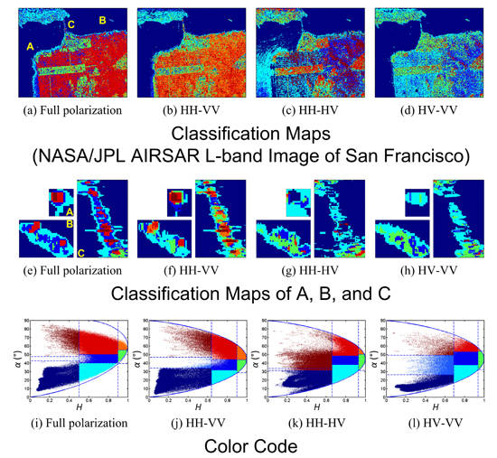
The classification map of fully polarimetric San Francisco data using Cloude-Pottier decomposition is shown in Figure 9a, with the color code in Figure 4b. Figure 4b is plotted again in Figure 9e for clarity. The classification maps of the corresponding HH-VV, HH-HV, and HV-VV data using the modified Cloude-Pottier decomposition are shown in Figure 13b–d, with the color code in Figure 13f–h. The size of the filtering windows is N=5 herein. The corresponding scattering mechanism retention ratios are listed in Table 7.

Table 7. Scattering mechanism retention ratios R_r (%) of AIRSAR San Francisco data.

	Z1	Z2	Z3	Z4	Z5	Z6	Z8	Z9	Average
HH-VV	99.46	86.92	90.20	55.82	21.90	45.03	64.05	83.59	68.37
HH-HV	77.75	0	57.38	35.42	19.89	5.67	38.52	10.82	30.68
HV-VV	99.52	25.38	19.71	39.64	17.45	2.95	70.57	3.10	34.79

Table 7. Scattering mechanism retention ratios R_r (%) of AIRSAR San Francisco data.

	Z1	Z2	Z3	Z4	Z5	Z6	Z8	Z9	Average
HH-VV	99.46	86.92	90.20	55.82	21.90	45.03	64.05	83.59	68.37
HH-HV	77.75	0	57.38	35.42	19.89	5.67	38.52	10.82	30.68
HV-VV	99.52	25.38	19.71	39.64	17.45	2.95	70.57	3.10	34.79

Terrains with different scattering mechanisms, such as sea terrain with low entropy surface scattering, mountain terrain with medium entropy surface scattering, buildings with medium entropy multiple scattering, and forests with high entropy dipole scattering, can be effectively discriminated by Cloude-Pottier decomposition for fully polarimetric applications, as shown in Figure 9a.

Figure 9. Classification maps of AIRSAR San Francisco data (N = 5). (a) Full polarization; (b) HH-VV; (c) HH-HV; (d) HV-VV; (e) Color code for full polarization; (f) Color code for HH-VV; (g) Color code for HH-HV; (h) Color code for HV-VV.

Figure 9. Classification maps of AIRSAR San Francisco data (N = 5). (a) Full polarization; (b) HH-VV; (c) HH-HV; (d) HV-VV; (e) Color code for full polarization; (f) Color code for HH-VV; (g) Color code for HH-HV; (h) Color code for HV-VV.

Figure 9 and Table 7 show that the performance of HH-VV SAR for extracting scattering mechanisms exceeds those of HH-HV and HV-VV SARs. Four terrains can also be classified by the modified Cloude-Pottier decomposition for HH-VV SAR data. Moreover, the extraction performance for sea, mountains, forests, and mid-right 45° buildings is comparable with that of fully polarimetric SAR. The average retention ratio of HH-VV is 68.37%, and the corresponding values for HH-HV and HV-VV are nearly half of that value. Only the retention ratios of Z5 and Z6 are less than 50% for HH-VV. This indicates the following: (1) the medium entropy dipole scatters (blue) of the building area and lower left coast in Figure 9a become other mechanisms in Figure 9b; and (2) the medium entropy multiple scatters (red) of the city in Figure 9a become high entropy multiple scatters (orange) in Figure 9b.

Compared with Figure 9b, Figure 9c,d illustrate that the performance of the extracting scattering mechanism for HH-HV and HV-VV SARs is worse. Although four terrains can be differentiated, the scattering mechanisms are greatly confused. Only the retention ratios of Z1 and Z3 are higher than 50% for HH-HV in Table 7. Correspondingly, the low entropy surface scatters of the upper sea area in Figure 9c are acceptable. However, the low entropy multiple scatters of the building area in Figure 9c are higher than those in Figure 9a due to other scatters transferring into Z3. Only the retention ratios of Z1 and Z8 are higher than 50% for HV-VV. Consequently, the low entropy surface scatters of the sea area and high entropy dipole scatters of the forest area in Figure 9d are acceptable. Furthermore, HH-HV and HV-VV SARs poorly extract other scattering mechanisms.

Mile Rock, Alcatraz Island, and the Golden Gate Bridge are indicated by A, B, and C in Figure 9a, respectively. More detailed images of these areas are provided below. A flat-roofed, cylindrical lighthouse is the only building at Mile Rock. The roof is set up as a helipad. There are several low buildings, a water tower, and a lighthouse on Alcatraz Island. The Golden Gate Bridge is composed of a deck, two piers, and many cables. The basic scattering mechanisms of the three objects are well extracted by HH-VV SAR. In particular, low and medium entropy multiple scattering mechanisms, denoting polyhedral characteristics of buildings, are identified by HH-VV SAR and fully polarimetric SAR, whereas HH-HV and HV-VV SARs cannot extract the crucial scattering mechanisms of the three targets.

(2)

E-SAR Oberpfaffenhofen data

The No. 11 and No. 18 training datasets in Table 1 are L-band 1-look data of Oberpfaffenhofen and C-band 8-look data of San Francisco acquired by DLR E-SAR and CSA-MDA RADARSAT-2, respectively, as shown in Figure 10.

Figure 10. Color-coded Pauli reconstructed and Google Earth images of No. 11 and No. 18 training data. (a) No. 11, E-SAR Oberpfaffenhofen data; (b) No. 18, RADARSAT-2 San Francisco data.

Figure 10. Color-coded Pauli reconstructed and Google Earth images of No. 11 and No. 18 training data. (a) No. 11, E-SAR Oberpfaffenhofen data; (b) No. 18, RADARSAT-2 San Francisco data.

An airport, farmland, and various buildings are shown in Figure 10a. The terrains in Figure 10b are the same as those in Figure 4a: sea, mountains, forests, and buildings.

The classification maps of the full- and dual-polarization Oberpfaffenhofen data using Cloude-Pottier decomposition and the modified version are shown in Figure 11a–d, with the color code in Figure 11e–h. The size of the filtering windows is N=9. The corresponding scattering mechanism retention ratios are listed in Table 8.

Table 8. Scattering mechanism retention ratios R_r (%) of E-SAR Oberpfaffenhofen data.

	Z1	Z2	Z3	Z4	Z5	Z6	Z8	Z9	Average
HH-VV	80.64	95.59	85.14	46.97	56.67	48.33	61.90	74.21	68.68
HH-HV	61.17	0	16.65	76.27	15.20	13.29	55.36	12.53	31.31
HV-VV	61.03	8.68	11.10	56.92	21.20	16.69	45.66	1.53	27.85

Table 8. Scattering mechanism retention ratios R_r (%) of E-SAR Oberpfaffenhofen data.

	Z1	Z2	Z3	Z4	Z5	Z6	Z8	Z9	Average
HH-VV	80.64	95.59	85.14	46.97	56.67	48.33	61.90	74.21	68.68
HH-HV	61.17	0	16.65	76.27	15.20	13.29	55.36	12.53	31.31
HV-VV	61.03	8.68	11.10	56.92	21.20	16.69	45.66	1.53	27.85

The performance of HH-VV SAR for extracting scattering mechanisms is closest to that of fully polarimetric SAR, with an average retention ratio of 68.68% in Table 8; the majority of scatters are correctly discriminated in Figure 11b. However, the majority of scatters are assigned incorrect labels by HH-HV and HV-VV SARs in Figure 11c,d, and the retention ratios are less than half of that of HH-VV SAR.

Figure 11. Classification maps of E-SAR Oberpfaffenhofen data (N = 9). (a) Full polarization; (b) HH-VV; (c) HH-HV; (d) HV-VV; (e) Color code for full polarization; (f) Color code for HH-VV; (g) Color code for HH-HV; (h) Color code for HV-VV.

Figure 11. Classification maps of E-SAR Oberpfaffenhofen data (N = 9). (a) Full polarization; (b) HH-VV; (c) HH-HV; (d) HV-VV; (e) Color code for full polarization; (f) Color code for HH-VV; (g) Color code for HH-HV; (h) Color code for HV-VV.

Several objects are denoted by D, E, F, and G in Figure 11a. These objects are magnified in the images below. Area D, labeled as medium entropy surface scattering, is clearly presented in Figure 11a. It is confused with area E in Figure 11b because the medium entropy surface scattering diffuses to the medium entropy dipole scattering mechanism in area D. The scattering mechanisms of areas D and E are differently labeled such that the two areas can be discriminated.

The five visible targets with dominate low entropy multiple scattering in area F in Figure 11a are correctly and clearly displayed by HH-VV SAR in Figure 11b. These targets are set apart with false scattering mechanisms, low entropy surface scattering, in Figure 11c. They cannot be differentiated from the background in Figure 11d.

The target with low entropy surface scattering in area G is labeled with the correct mechanism in Figure 11b. The contour of the target is clear, whereas the scattering mechanism is incorrect in Figure 11c,d.

(3)

RADARSAT-2 San Francisco data

The classification maps of the full- and dual-polarization RADARSAT-2 San Francisco data using Cloude-Pottier decomposition and the modified version are shown in Figure 12a–d, with the color code in Figure 12e–h. The size of the filtering windows is N=5. The scattering mechanism retention ratios are listed in Table 9.

Figure 12. Classification maps of RADARSAT-2 San Francisco data (N = 5). (a) Full polarization; (b) HH-VV; (c) HH-HV; (d) HV-VV; (e) Color code for full polarization; (f) Color code for HH-VV; (g) Color code for HH-HV; (h) Color code for HV-VV.

Figure 12. Classification maps of RADARSAT-2 San Francisco data (N = 5). (a) Full polarization; (b) HH-VV; (c) HH-HV; (d) HV-VV; (e) Color code for full polarization; (f) Color code for HH-VV; (g) Color code for HH-HV; (h) Color code for HV-VV.

Table 9. Scattering mechanism retention ratios R_r (%) of RADARSAT-2 San Francisco data.

	Z1	Z2	Z3	Z4	Z5	Z6	Z8	Z9	Average
HH-VV	99.61	74.61	73.90	68.89	22.99	59.20	72.01	67.74	67.37
HH-HV	98.69	0	5.36	30.38	2.23	4.41	69.32	7.44	27.23
HV-VV	99.45	3.40	2.44	29.05	8.70	3.83	73.16	0.94	27.62

Table 9. Scattering mechanism retention ratios R_r (%) of RADARSAT-2 San Francisco data.

	Z1	Z2	Z3	Z4	Z5	Z6	Z8	Z9	Average
HH-VV	99.61	74.61	73.90	68.89	22.99	59.20	72.01	67.74	67.37
HH-HV	98.69	0	5.36	30.38	2.23	4.41	69.32	7.44	27.23
HV-VV	99.45	3.40	2.44	29.05	8.70	3.83	73.16	0.94	27.62

In Figure 12, four terrains are identified by both full-polarization and HH-VV SARs. HH-HV and HV-VV SARs cannot obtain the correct scattering mechanisms, except in the sea area.

Only the retention ratio of Z5 is lower than 50% for HH-VV in Table 9. Consequently, medium entropy dipole scatters (blue) of the mountain, forest, and building areas are set to other mechanisms in Figure 12b. The retention ratios of the seven other zones are higher than 50%. Therefore, Figure 12b is similar to Figure 12a.

There are six zones with retention ratios of less than 50% for HH-HV and HV-VV SARs, and five retention ratios are less than 10%. The retention ratios of Z1 and Z8 exceed 50%; thus, low entropy surface scattering of the sea area and high entropy dipole scattering of the mountain and forest areas are preserved in Figure 12c,d. However, many scatters of the building area are labeled as low entropy surface scattering. This observation indicates that the building and sea areas are confused. Furthermore, marking most scatters of the mountain and forest areas as high entropy dipole scattering prevents the two terrains from being differentiated. Thus, the scattering mechanisms of the mountain, forest, and building areas in Figure 12c,d are considerably different from those in Figure 12a.

Mile Rock, Alcatraz Island, and the Golden Gate Bridge remain marked by A, B, and C in Figure 12a. More detailed images of these areas are provided below. The scattering mechanism extraction performance of HH-VV SAR for Mile Rock, Alcatraz Island, and the Golden Gate Bridge is close to that of fully polarimetric SAR. The performance of HH-HV and HV-VV SARs for extracting scattering mechanisms for the three targets is considerably worse. Low and medium entropy multiple scatters of Alcatraz Island and the Golden Gate Bridge are not adequately discriminated; moreover, the three-parallel scatter of the Golden Gate Bridge is converted into one- or two-parallel scatter in Figure 12c,d, respectively.

Two clear differences in the scattering mechanism extraction for Mile Rock and the Golden Gate Bridge can be noted when comparing Figure 12 with Figure 9.

First, the scattering mechanisms of Mile Rock are low and medium entropy multiple scattering and medium entropy surface and dipole scattering in Figure 9a,b. The multiple scattering is from the lighthouse body and the dihedral formed by the body and base. However, only medium entropy surface scattering is observed for Mile Rock in Figure 12a,b, with no multiple scattering being extracted, even in several further experiments using different window sizes. This may be due to the imaging geometry.

Second, the Golden Gate Bridge appears as a thick line including low and medium entropy multiple scattering and medium entropy surface and dipole scattering in Figure 9a because the SAR sensor illuminated from the top of the image. Nevertheless, the bridge consists of three parallels in Figure 12a due to the sensor illuminating from the left of the image. The left parallel is from the bridge body, with dominant medium entropy multiple and dipole scattering and lower low entropy multiple and medium entropy surface scattering. The middle parallel is from the cables and bridge body, with only low and medium entropy multiple scattering. The right parallel is triple scattering from the bridge body and the sea with low α, including medium entropy surface and dipole scattering.

6. Conclusions

The modified Cloude-Pottier decomposition is used to analyze the performance of HH-VV, HH-HV, and HV-VV SARs for scattering mechanism extraction. We draw the following conclusions based on the theoretical and experimental results:

(1)

HH-VV SAR can discriminate scattering from an isotropic surface, horizontal dipole, and isotropic dihedral. Scatters diffuse to a small extent in the HH-VV H-α plane. Therefore, HH-VV SAR extracts the eight scattering mechanisms in the H-α plane with acceptable performance. Thus, HH-VV SAR is an alternative to fully polarimetric SAR. The average scattering mechanism retention ratios of the three images are higher than 67%. The decreased performance of HH-VV SAR for scattering mechanism extraction compared with that of full polarization is due to the lack of cross-polarization.

(2)

HH-HV and HV-VV SARs cannot separate surface, dipole, and multiple scattering mechanisms because of a lack of co-polarization. The distribution of scatters in the HH-HV and HV-VV H-α planes is quite different from that in the full-polarization H-α plan due to the scatters of most zones strongly diffusing and transferring in the HH-HV and HV-VV H-α planes. Thus, HH-HV and HV-VV SARs do not adequately extract scattering mechanisms in the H-α plane, indicating that co-polarization is vital for extracting scattering mechanisms.

This paper explores the performance of dual-polarization SARs for extracting scattering mechanisms. The performance is compared with that of fully polarimetric SAR. Comparison with compact SAR will be performed in the next investigation.