Mapping Forest Canopy Height over Continental China Using Multi-Source Remote Sensing Data

Abstract

Spatially-detailed forest height data are useful to monitor local, regional and global carbon cycle. LiDAR remote sensing can measure three-dimensional forest features but generating spatially-contiguous forest height maps at a large scale (e.g., continental and global) is problematic because existing LiDAR instruments are still data-limited and expensive. This paper proposes a new approach based on an artificial neural network (ANN) for modeling of forest canopy heights over the China continent. Our model ingests spaceborne LiDAR metrics and multiple geospatial predictors including climatic variables (temperature and precipitation), forest type, tree cover percent and land surface reflectance. The spaceborne LiDAR instrument used in the study is the Geoscience Laser Altimeter System (GLAS), which can provide within-footprint forest canopy heights. The ANN was trained with pairs between spatially discrete LiDAR metrics and full gridded geo-predictors. This generates valid conjugations to predict heights over the China continent. The ANN modeled heights were evaluated with three different reference data. First, field measured tree heights from three experiment sites were used to validate the ANN model predictions. The observed tree heights at the site-scale agreed well with the modeled forest heights (R = 0.827, and RMSE = 4.15 m). Second, spatially discrete GLAS observations and a continuous map from the interpolation of GLAS-derived tree heights were separately used to evaluate the ANN model. We obtained R of 0.725 and RMSE of 7.86 m and R of 0.759 and RMSE of 8.85 m, respectively. Further, inter-comparisons were also performed with two existing forest height maps. Our model granted a moderate agreement with the existing satellite-based forest height maps (R = 0.738, and RMSE = 7.65 m (R² = 0.52, and RMSE = 8.99 m). Our results showed that the ANN model developed in this paper is capable of estimating forest heights over the China continent with a satisfactory accuracy. Forth coming research on our model will focus on extending the model to the estimation of woody biomass.

1. Introduction

Forests play a key role in the global climate system and carbon cycle. Forests store carbon in their above- and below-ground biomass [1]. As an important predictor of forest biomass and carbon stock, the vertical structure of forests has been well monitored in previous studies [2,3,4]. Light detection and ranging (LiDAR) remote sensing, is useful in the large-scale investigations of forest structural attributes, such as forest canopy height [2,5,6,7,8,9,10].

In recent years, LiDAR instruments have demonstrated their capability to estimate forest heights [11]. For instance, the Geoscience Laser Altimeter System (GLAS) on board the Ice, Cloud and Land Elevation Satellite (ICESat) has provided within-footprint height measures at the global scale [2,5,12]. However, the lack of valid GLAS data in some regions is problematic. Because the GLAS data are spatially incomplete, multiple geospatial predictors were supplemented to obtain spatially-continuous forest height maps in recently-published approaches [2,3,5,13]. In addition, the GLAS data are highly sensitive to topographic features due to its large footprint size, which causes overestimations of forest height [14]. In this paper, in order to solve those two problems degrading the accuracy of GLAS-based forest height maps, we proposed a new approach based on the artificial neural network (ANN).

The principal method was to combine GLAS derived tree heights with ancillary variables in the ANN model and then to produce a wall-to-wall forest height map over the China continent. Selected geospatial predictors were a series of climate variables, elevation, vegetation cover and multispectral reflectance data from the Moderate Resolution Imaging Spectroradiometer (MODIS). We resampled all of the input predictors to obtain the final output map of forest heights at a 1-km spatial resolution.

2. Materials and Methods

2.1. Data and Processing

2.1.1. ICESat Data and Processing

The ICESat/GLAS is the first spaceborne LiDAR system, which was designed to obtain characteristics of the Earth’s surface structures with unprecedented accuracy [15]. The ICESat/GLAS data can provide information related to land surface elevation with a spatial resolution of 70 m (ellipsoidal footprints) and 170 m spaced intervals [16]. The global ICESat/GLAS data are available for a period spanning from 2003 to 2008 [17]. Due to the short lifetime of GLAS, altimetry information was collected only in the following months: February–March, May–June, and October–November [11,18]. There are totally 15 GLAS data products including Level-1 and Level-2 that were disseminated by the NSIDC (National Snow and Ice Data Center). The GLA14 used in this study is an GLAS Level-2 Land Surface Altimetry product that provides information on surface elevations, laser footprint geolocation, waveform parameters and reflectance, as well as geodetic, instrument, and atmospheric corrections for range measurements. In previous studies, the GLA14 product has been used to estimate forest canopy heights within each footprint [1,19].

In this study, we obtained the GLAS data recorded from May to October (2003–2006), because these data represent the approximated growing season and thus, the best leaf-on condition of forests. In our analyses, GLAS footprints over non-forest area were excluded. We further screened invalid GLAS data using several preprocessing filters in order to reduce the impact of slope gradient, atmospheric forward scattering, signal saturation and cloud contamination [14,20,21]. The GLAS data were considered valid when footprints were located over the forest classes in the land cover (LC) map with >50% tree cover percent in the vegetation continuous field (VCF). Then, the quality of GLAS shots over the forested area was investigated using GLA14 waveform parameters regarding the cloud, signal saturation and atmospheric forward scattering [1,21,22]. Firstly, we removed the invalid GLAS footprints affected by signal saturation and atmospheric forward scattering based on the internal flags (“FRir_qaFlag = 15” and “satNdx = 0”) GLA14 product contained [20,21,22]. To further remove waveforms with signal dominated by low cloud, we just selected the waveforms based on the filter that was built by using the absolute difference (50 m) between ASTER DEM and the internal elevation value from GLA14 product [21]. The terrain slope gradient also impacts the quality of the GLAS data [23]. In order to minimize the bias resulting from the terrain slope, we filtered the GLAS shots where the terrain slope is higher than 10 degrees [24].

2.1.2. Land Surface Reflectance

The land surface reflectance data used in this study were acquired from the MCD43B4 which is a product of the MODIS nadir bidirectional reflectance distribution function adjusted reflectance (NBAR) with a spatial resolution of 1 km [25]. The NBAR product represents the best characterization of surface reflectance over a 16-day period. In the study, seven spectral bands in the MCD43B4 averaged over the approximated growing season (June-September) between 2004 and 2006 were extracted at a 1-km spatial resolution.

2.1.3. Climate Data

Weather station-based climatic variables, precipitation and temperature, were derived from China Meteorological Data Sharing Service System (CMDSSS). There are total of 754 weather stations that can provide annual meteorological records. The precipitation and temperature data covered a time period from 2004 to 2006. For each weather station, 3-year averaged precipitation and temperature were obtained. Then, we interpolated these two climate variables using ordinary kriging to generate the gridded maps of annual average precipitation and temperature [26].

2.1.4. Ancillary Data

Ancillary data applied in this study involved the digital elevation model (DEM), LC, and VCF. The DEM data were obtained from the Advanced Spaceborne Thermal Emission and Reflection Radiometer (ASTER) Global DEM (GDEM V2) of which spatial resolution is 30 m [27]. The use of DEM data is first to remove invalid GLAS shots with a signal contaminated by low clouds and second to generate a gridded map of slope at the same spatial resolution of the GDEM V2 data (30 m). This continuous field of slope was used to correct the GLAS derived tree heights based on the terrain correction method [21].

The LC data were derived from a MODIS global LC product (MCD12Q1, 500-m grid). Additionally, the VCF data were also obtained from the MODIS (MOD44B, 250-m grid). We selected the International Geosphere-Biosphere Programme (IGBP) of the LC and tree cover percent of the VCF over China for the year 2005 [28].

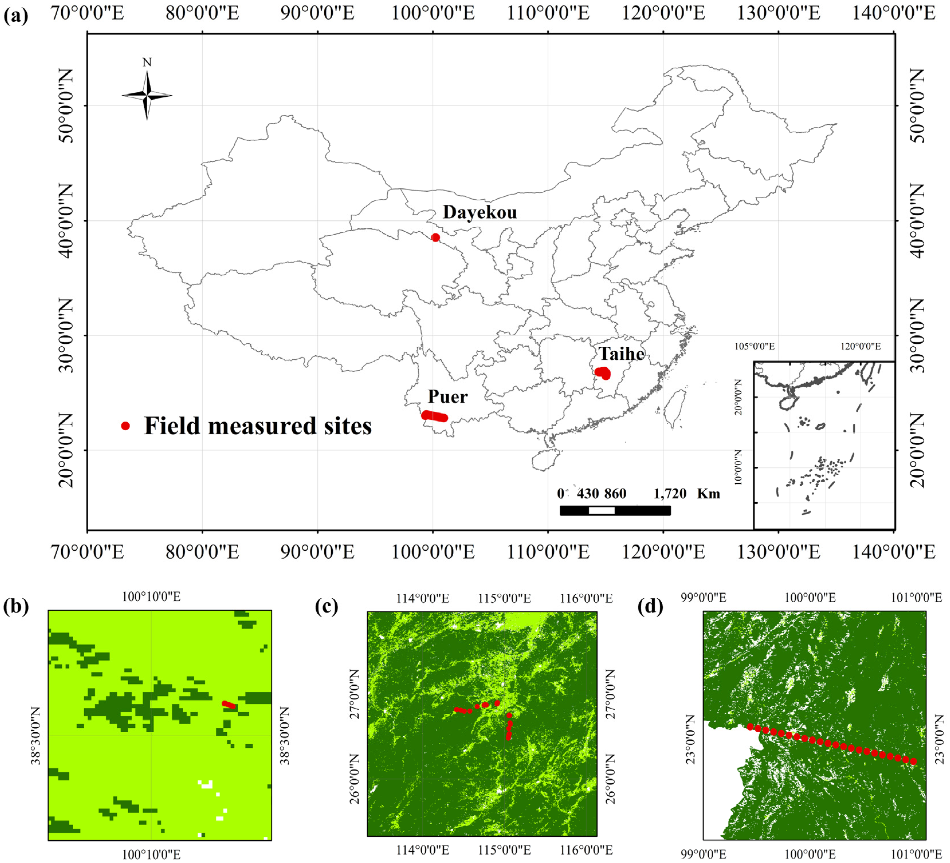
2.1.5. Field-Measured Tree Heights

Field-measured tree heights were used to evaluate our modeled tree heights. We chose 92 plots from three experimental sites. These three field regions are located in Gansu (northwestern China), JiangXi (southern China) and Yunnan (southwestern China), respectively.

The location of the filed experimental regions and corresponding plots is shown in Figure 1. The detailed information on the field sites is delivered in Table 1. Plots in the field sites were selected according to the definition of forest area using LC and VCF in this study. The field measured tree heights were averaged for each plot.

Table 1. The detailed information on three field experiment regions.

Sites	Number of Plots	Plot Size (m)	Acquisition Year	Forest Type	References
Dayekou, Gansu	36	20 × 20, 25 × 25	2008	Picea Crassifolia	[29]
Taihe, Jiangxi	22	50 × 50	2012	Masson pine, Slash Pine
Puer, Yunnan	34	15 × 15	2013	Pinus Kesiya, Fir, Eucalyptus

Table 1. The detailed information on three field experiment regions.

Sites	Number of Plots	Plot Size (m)	Acquisition Year	Forest Type	References
Dayekou, Gansu	36	20 × 20, 25 × 25	2008	Picea Crassifolia	[29]
Taihe, Jiangxi	22	50 × 50	2012	Masson pine, Slash Pine
Puer, Yunnan	34	15 × 15	2013	Pinus Kesiya, Fir, Eucalyptus

Figure 1. Field measurement sites. (a) Distribution of three field measurement regions; (b) Dayekou field sites in Gansu; (c) Taihe field sites in Jiangxi; (d) Puer field sites in Yunnan; (b–d) the background color map represents the MODIS land cover (LC) forest types.

Figure 1. Field measurement sites. (a) Distribution of three field measurement regions; (b) Dayekou field sites in Gansu; (c) Taihe field sites in Jiangxi; (d) Puer field sites in Yunnan; (b–d) the background color map represents the MODIS land cover (LC) forest types.

2.2. Methods

2.2.1. GLAS Tree Height Estimation

The GLAS tree heights were used as training data to build the ANN model for tree height estimation and to validate model performances. GLAS height metrics were extracted based on the “decomposition of GLAS waveforms into multiple Gaussian distribution curves” as described in previous studies [18,19,30]. The direct method was used to estimate canopy height based on the vertical difference between the signal start point and the ground peak. The signal start point was provided in the GLA14 product (i_SigBegOff). Also, the GLA14 product contains up to six Gaussian peaks for each GLAS waveform (i_gpCntRngOff). The distance between “i_SigBegOff” and “i_gpCntRngOff” represents the waveform metric RH100 (100% energy return height) of GLAS-derived tree height estimation [9,17]. Because the RH100 can be potentially affected by the topographic gradient [20], we applied the topographic correction approach [14,21] to obtain more accurate GLAS tree heights. The calculation formula of GLAS-derived tree heights based on topographic correction is shown as Equation (1),

$$H_{GLAS}=\left(D_{SigBegOff}-D_{gpCntRngOff}\right)-\frac{d\text{*}\tan \theta }{2}$$

(1)

where H_GLAS represents the GLAS derived tree heights, D_sigBegoff and D_gpcntRngoff separately represent the values of the beginning signal and the ground peak of the GLAS full-waveform, d is the GLAS footprint size of 70 m [3,16], and θ is the topographic slope.

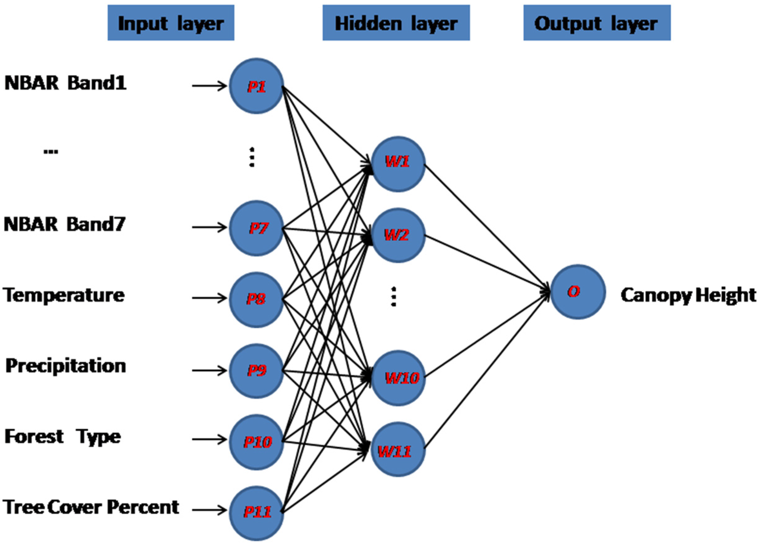
2.2.2. Tree Height Modeling

We employed the ANN algorithm to combine the GLAS-derived tree heights with the geospatial predictors. The neural network algorithms are products of artificial intelligence as black-box models, and the first prototype neural network was proposed in 1943 [31]. To date, more than 30 different neural network models have been developed [32], which have been widely used in various fields [33]. Here, we used the feed-forward neural network (FFNN) algorithm for the forest height predictions. The selected model consisted of 11 neurons in the input layer, 11 neurons in the hidden layer and 1 neuron in the output layer. The 11 parameters in the input layer include the LC class, VCF tree cover percent, temperature, precipitation, and seven MODIS NBAR bands. All of the 11 parameters in the input layer are related to forest growth, distribution or the characteristics’ expression. The neuron in the output layer refers to the modeled forest canopy heights. Figure 2 depicts the schematic diagram of the ANN model proposed in this study.

Figure 2. The schematic diagram of the ANN model proposed in this study. There are 11 neurons in the input layer, 11 neurons in the hidden layer and 1 neuron in the output layer.

Figure 2. The schematic diagram of the ANN model proposed in this study. There are 11 neurons in the input layer, 11 neurons in the hidden layer and 1 neuron in the output layer.

To train the ANN model, we applied the back-propagation (BP) process algorithm to train the neural networks [34]. For each pixel, we trained the FFNN to estimate forest canopy heights. Based on the temperature and precipitation values, 15 pairs of training data were chosen to train the FFNN while 5 validation pairs remained to prevent the over-fitting of the FFNN. The selection discipline of training and validation data pairs is to obtain 20 GLAS shots that are located in the most similar climatic condition factor (temperature and precipitation) based on Equation (2),

$$D_i={\left(\frac{T_{pix}-T_i}{T_{max}-T_{min}}\right)}^2+{\left(\frac{P_{pix}-P_i}{P_{max}-P_{min}}\right)}^2$$

(2)

where D_i is the distance of the climate variable difference between the reference pixel of the canopy height estimation map and the i-th GLAS shot; T_pix is the temperature value of the reference pixel; T_i is the temperature value of i-th GLAS shot; T_pix is the precipitation value of the reference pixel; P_i is the precipitation value of the i-th GLAS shot; T_max and P_max are respectively the maximum values of temperature and precipitation values over continental China, and T_min and P_min are respectively the minimum values of temperature and precipitation values over the continental China.

After selecting the training and validation data pairs for a pixel, the network gets trained by the training data until the FFNN model loses its best performance given validation data. Then, the trained FFNN model was used for estimating the forest canopy height over the target pixel.

2.2.3. Error Analysis

To assess the performance of the canopy height model in the study, we prepared several reference datasets. These datasets mainly include field-measured tree heights, GLAS-derived tree heights and existing forest height products. The root mean square error (RMSE) was calculated using the following Equation (3):

$$RMSE \left(m\right)=\sqrt{\frac{{{\displaystyle \sum }}_{i=1}^N{\left(H_{Predicted}-H_{Ref}\right)}^2}{N}}$$

(3)

where, H_predicted is the predicted heights derived from the model; and H_Ref is the validation heights derived from the reference datasets which were used to validate the predicted tree heights.

2.2.4. Calibration and Comparison with Existing Canopy Height Products

In this study, we present three forms of validation. One is the field calibration of the modeled tree heights, which was based on the field measurements mentioned in Section 2.1.5. For each field plot, we averaged all tree heights to obtain the representative height of this plot. The pixel on the modeled height map that is closest to the field plot centroid was chosen for the validation. The second is that the modeled heights were directly evaluated with the footprint-level GLAS heights (footprint vs. modeled pixel). The third is wall-to-wall map validation from the interpolated GLAS tree height map. Here, we averaged the GLAS tree heights from 20 GLAS shots selected according to Equation (2) to produce a full gridded map. Then, pixel-to-pixel comparisons (FFNN vs. averaged GLAS tree heights) were performed.

Lastly, we compared our modeled tree height map with two existing forest height products. These two reference products are named H_Simrad and H_Ni, respectively, following their creators Simard and Ni [2,3]. Our modeled data and two reference products commonly provide forest canopy heights over the continental China, but their modeling strategies are significantly different. We also calculated and discussed the differences between our modeled height map and the two reference products in a view of the different canopy height modeling approaches.

3. Results and Discussion

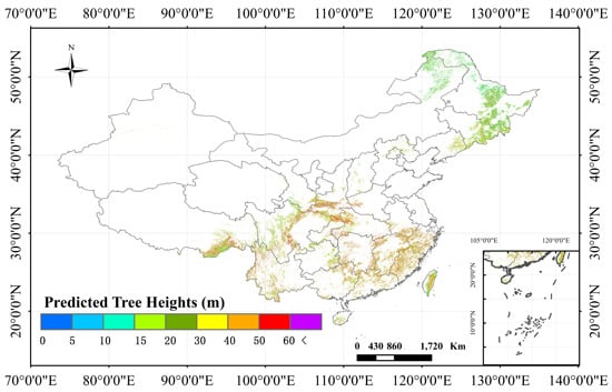
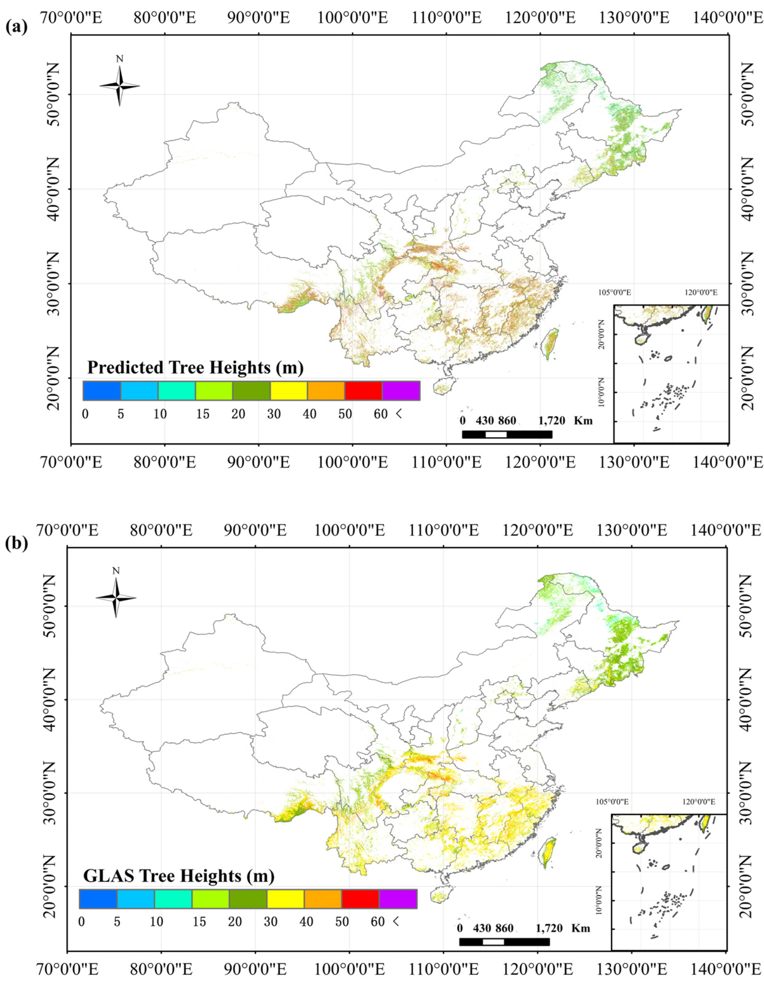
3.1. Canopy Height Map in China

A contiguous map of canopy heights with a spatial resolution of 1 km over the continental China was generated from the FFNN using the gridded geospatial predictors (Figure 3a). This map (mean = 36.44 m, Figure 3a) showed a good consistency with the spatial pattern of GLAS tree heights (mean = 30.00 m, Figure 3b).

Figure 3. Maps of modeled and averaged GLAS-derived tree heights over continental China at 1-km spatial resolution. (a) The modeled height map using the trained ANN model proposed in this paper; (b) GLAS tree height map. The GLAS tree height map is made from the interpolation of the averaged GLAS-derived tree heights.

Figure 3. Maps of modeled and averaged GLAS-derived tree heights over continental China at 1-km spatial resolution. (a) The modeled height map using the trained ANN model proposed in this paper; (b) GLAS tree height map. The GLAS tree height map is made from the interpolation of the averaged GLAS-derived tree heights.

From the estimation result of canopy heights over China, we can see that relatively tall trees were growing in the central and southern regions (Sichuan, Hubei, Yunnan and Chongqing). The trees distributed in the Northern China show obviously lower heights than those in Southern regions. Specially, the forests distributed in Heilongjiang and East of Inner Mongolia province, which are close to the border of Russia, have the lowest tree heights. The varying distribution of tree heights over China likely captures climate gradients. However, further assessment is still needed for exploring the underlying patterns of the tree height distribution.

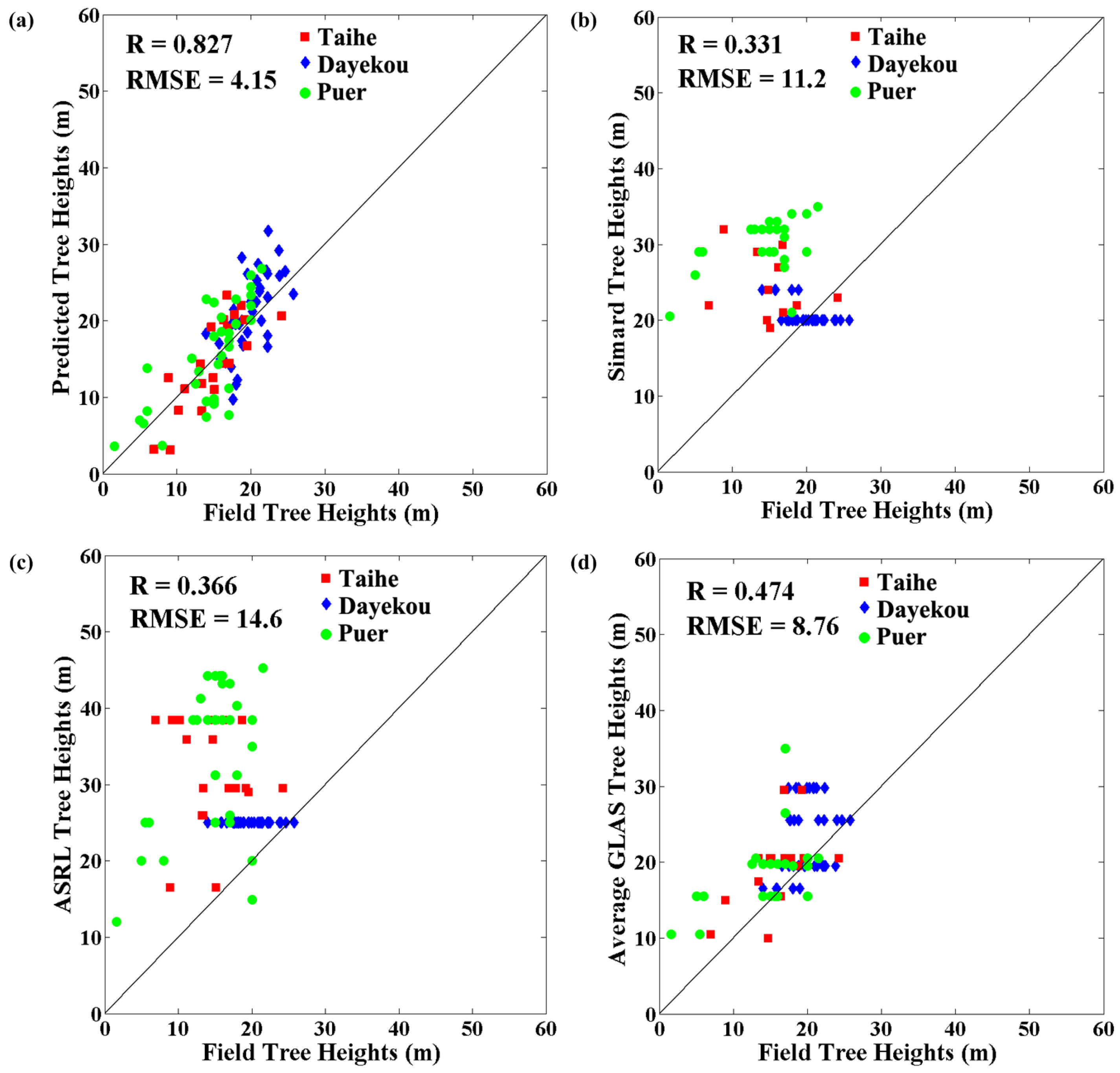
3.2. Ground Validation and Error Analysis

92 field plots were used in comparison with the FFNN-modeled tree heights. The validation showed a good agreement between the modeled and field-measured tree heights (Figure 4a). In order to show the outperformance of our model with respect to previous studies, we also evaluated H_Simrad, H_Ni and the GLAS tree height map produced from 20 GLAS shots selected according to Equation (2). From these comparison results (Figure 4b–d), we can see that the modeled heights have better accuracy than other approaches.

Figure 4. Ground validation result of the modeled tree heights, H_Simrad, H_Ni and GLAS tree height map. (a) The comparison between modeled tree heights and field measured tree heights; (b) The comparison between H_Simrad and field measured tree heights; (c) The comparison between H_Ni and field measured tree heights; (d) The comparison between averaged GLAS tree heights and field measured tree heights.

Figure 4. Ground validation result of the modeled tree heights, H_Simrad, H_Ni and GLAS tree height map. (a) The comparison between modeled tree heights and field measured tree heights; (b) The comparison between H_Simrad and field measured tree heights; (c) The comparison between H_Ni and field measured tree heights; (d) The comparison between averaged GLAS tree heights and field measured tree heights.

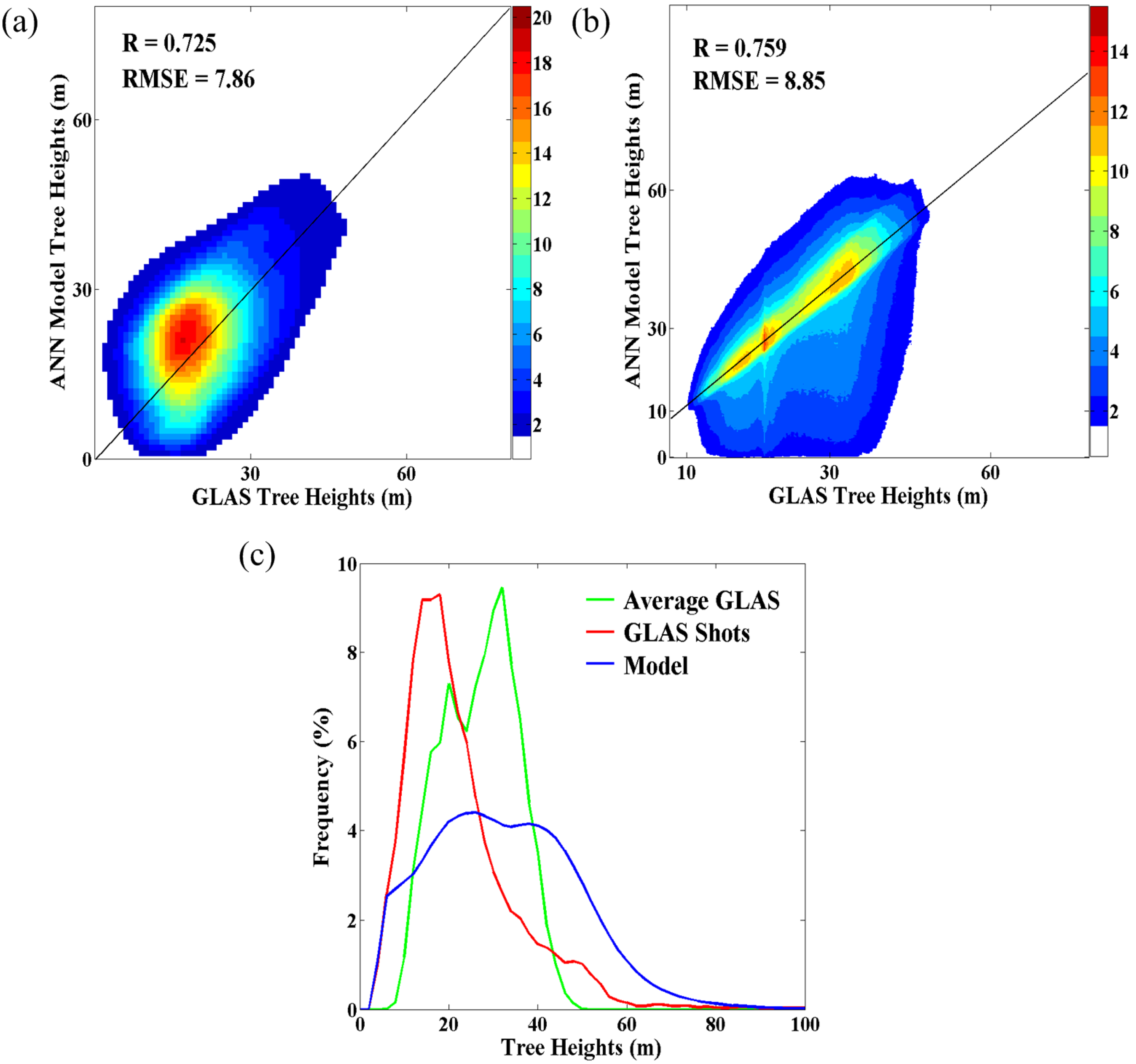
3.3. Actual GLAS-Derived Tree Height Validation and Error Analysis

The modeled heights from the FFNN at the continental China scale were also evaluated using the GLAS-derived heights. This validation was based on two types of GLAS metrics, including the footprint-level GLAS heights and a full gridded GLAS height map.

Figure 5. The comparison results between modeled tree heights and actual GLAS derived tree heights. (a) The comparison between modeled tree heights and discrete GLAS tree heights; (b) the comparison between modeled tree heights and averaged GLAS tree heights; (c) statistical characteristics of modeled tree heights, discrete GLAS tree heights and averaged GLAS tree heights.

Figure 5. The comparison results between modeled tree heights and actual GLAS derived tree heights. (a) The comparison between modeled tree heights and discrete GLAS tree heights; (b) the comparison between modeled tree heights and averaged GLAS tree heights; (c) statistical characteristics of modeled tree heights, discrete GLAS tree heights and averaged GLAS tree heights.

Both types of validation showed a consistency agreement between the FFNN modeled and GLAS height metrics (R = 0.725, RMSE = 7.86 m for the footprint-to-pixel level; R = 0.759, RMSE = 8.85 for the pixel-to-pixel level; Figure 5). However, Figure 5a depicts some difference between the model tree heights and footprint-to-pixel-level tree heights derived from GLAS shots. The main reason is that tree heights model in this study were trained from 20 GLAS shots which were selected according to Equation (2), including 15 training data and five validation data. As for one GLAS shot location (l_pix), these 20 GLAS shots for training and validating the tree height model should have the most similar temperature and precipitation with the GLAS shot location (l_pix). Additionally, the GLAS shot of location l_pix was included in the 20 GLAS shots. In general, modeled tree height should be similar to the GLAS shot height of location l_pix. When the temperature and precipitation of the GLAS shot location (l_pix) have a significant difference from the other 19 GLAS shots, the corresponding modeled tree height might be different from the GLAS shot height of location l_pix. Conversely, the modeled tree height is still similar to the mean value height of these 20 GLAS shots, which can explain the better consistency agreement in Figure 5b than in Figure 5a.

In order to further evaluate the modeled tree heights, we demonstrated the spatial distribution of deviations between the modeled and GLAS-derived heights. As shown in the map depicting the difference at the pixel-to-pixel level (Figure 6a), most forested pixels showed a moderate predictive power but overestimations were dominant over some regions.

Figure 6. The difference map of modeled tree heights with averaged GLAS tree heights.

Figure 6. The difference map of modeled tree heights with averaged GLAS tree heights.

The overestimation of tree heights tended to distribute over some special area where temperature is relatively low and precipitation is relatively high (e.g., east of Heilongjiang and Jilin, southeast of Tibet). The overestimation may be caused by the tree height model, which is more sensitive to the precipitation than temperature during the model training process. In addition, relatively high precipitation may have bigger impacts on forest trees’ growing and characteristics’ expression (leaf reflectance of forest tree) than a relatively low temperature, which might affect the accuracy of modeled tree heights. The specific reasons will be explored in a further study.

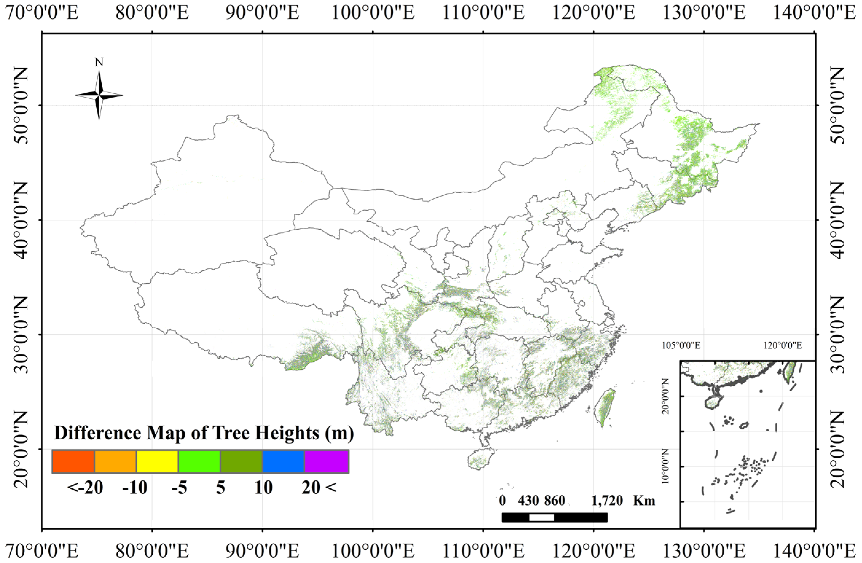
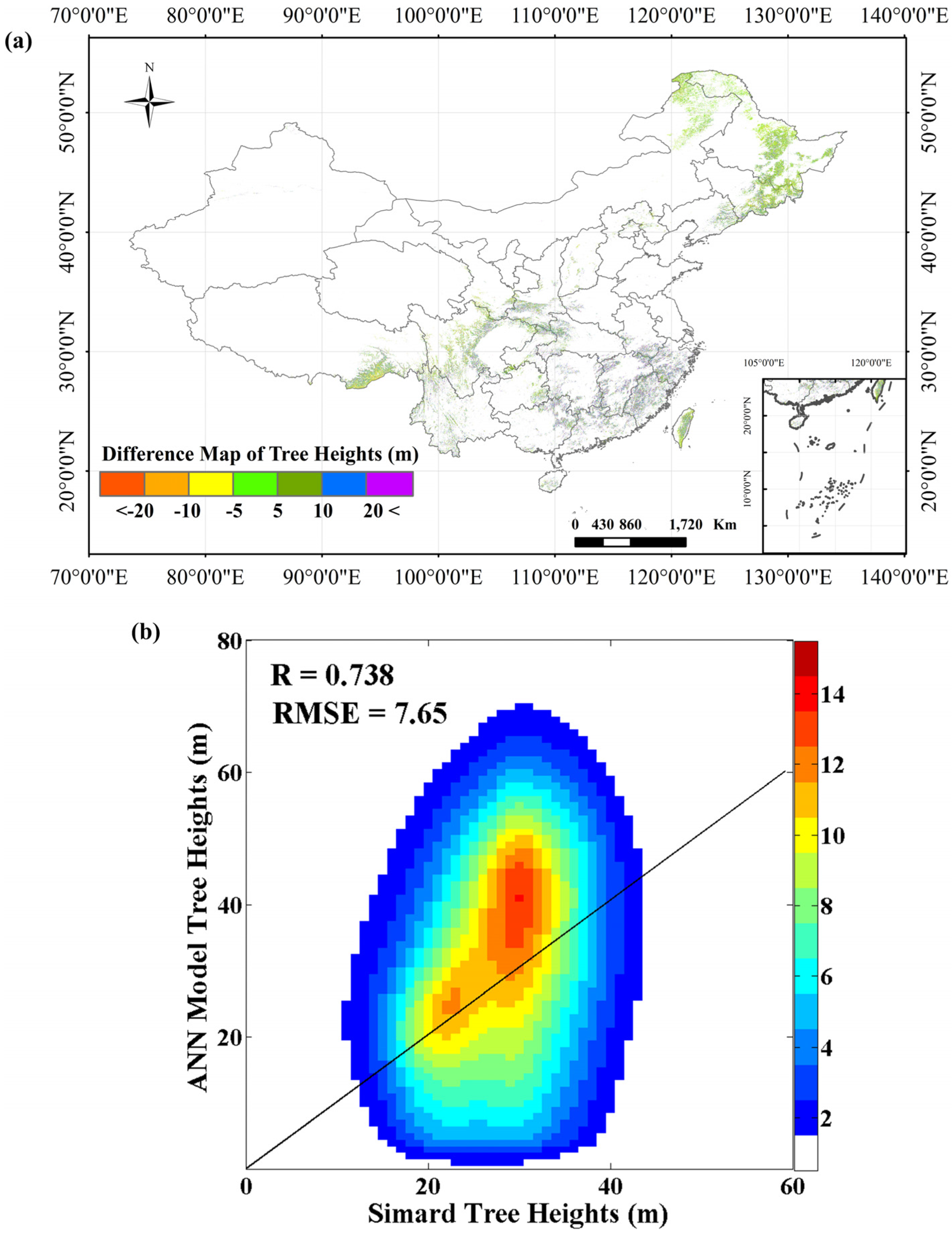
3.4. Comparison with Existing Tree Height Map

3.4.1. Comparison with Simard Tree Heights Map

Based on the definition of forest land area in this study, we obtained the pixel-to-pixel comparison result between our modeled heights and the H_simard. The difference map (Figure 7a) showed a moderate agreement. The differences were less generally 10 m.

From the comparison result (R = 0.738, RMSE = 7.65 m; Figure 7b), we can see a very good consistency between modeled tree heights and the $H_{Simard}$ when tree heights are less than 40 m. It is noteworthy that there are some obvious discrepancies existing where modeled tree heights are higher than 40 m. The disagreement between modeled tree heights and the $H_{Simard}$ for trees greater than 40 m might be caused by the following two reasons. On the one hand, the $H_{Simard}$ Simard tree heights are is the regional average height which made the forest height prediction result likely being less than 40 m. On the other hand, the overestimation of the modeled tree heights above 40min some places also appears to be an obvious disagreement with the $H_{Simard}$.

Figure 7. The comparison result between modeled tree heights and Simard tree heights. (a) The difference map of modeled tree heights with Simard tree heights; (b) the comparison between modeled tree heights and Simard tree heights.

Figure 7. The comparison result between modeled tree heights and Simard tree heights. (a) The difference map of modeled tree heights with Simard tree heights; (b) the comparison between modeled tree heights and Simard tree heights.

3.4.2. Inter-Comparison with Ni Tree Heights

Based on the climate zones defined by Ni [3], the comparison between the modeled heights and the H_Ni was conducted (Figure 8). As depicted in Figure 8a, the modeled heights and the H_Ni generally agreed. For the most of forest land area, the difference between the modeled heights and the H_Ni was less than 10 m. However, some regions in Southern China had relatively more significant difference, which might be caused by higher H_Ni values in this region.

Figure 8. The comparison result between the modeled tree heights and the H_Ni s. (a) The difference map of the modeled tree heights against H_Ni; (b) the comparison between the modeled tree heights and H_Ni.

Figure 8. The comparison result between the modeled tree heights and the H_Ni s. (a) The difference map of the modeled tree heights against H_Ni; (b) the comparison between the modeled tree heights and H_Ni.

The same comparison result was shown in Figure 8b (R² = 0.519, and RMSE = 8.99 m). In the case that the heights are less than 40 m, there is a good agreement between the modeled heights and the H_Ni. However, when the heights are higher than 40 m, the difference became larger. The main reason for these obvious errors is that in this process of comparison, we calculated the mean value of the modeled heights in climate zones, while the H_Ni is the maximum tree heights predicted from the optimized allometric scaling and resource limitation (ASRL) model as the height of the climate zone.

4. Concluding Remarks

The objective of this work was to predict the large-scale spatial pattern of forest heights over the continental China. The GLAS derived heights were used as an input for the model and as a result, a spatially-continuous forest height map was produced with a spatial resolution of 1000 m. Additional geospatial predictors were climatic variables (temperature and precipitation), forest type, tree cover percent and land surface reflectance. The approach was designed to train the artificial neural network (ANN) model to minimize the errors between GLAS-derived actual heights and model-derived forest heights. For each pixel of the forested land defined in the study, there was one ANN model to be trained and tested.

The ANN-modeled heights were firstly evaluated at the site scale. In three field experimental sites, regression analysis was performed to assess the correlation between the modeled and field-measured tree heights. The comparison showed a good agreement (n = 92, R = 0.827, and RMSE = 4.15 m). Meanwhile the modeled heights were assessed at the GLAS footprint-to-pixel level. We used more than thirty thousand GLAS shots for this evaluation. The comparison between the modeled and GLAS heights showed a reasonable correspondence (R = 0.725, and RMSE = 7.86 m).

In addition, the ANN modeled heights were compared with continuous forest height maps over the China continent. The comparison was firstly conducted with the interpolated GLAS height map. Their difference map showed that there were relatively small errors in the most Chinese forested lands (<10 m), and the ANN model tended to predict little higher tree heights than the gridded GLAS heights. Furthermore, the modeled tree heights were validated using the published products of tree heights (RMSE = 7.65 m, R = 0.738 for H_Simard; R² = 0.519, RMSE = 8.99 for H_Ni). According to the difference maps between the modeled and existing products, we obtained a small overestimation compared with the H_Simard and an underestimation compared with the H_Ni. These discrepancies could be mainly attributed to some inherent limitations of various tree height estimation approaches.

This paper reported the ANN model for the extensive forest canopy height predictions. The training method of the ANN model for each pixel successfully compensated for the limitations of previous tree height estimation approaches by using a single model in large-scale regions, which can greatly improve the accuracy of forest tree height estimation to some extent. As shown in the results, the trained ANN model in this article demonstrated a good performance in the estimation of tree heights over the continental China.

Nevertheless, the ANN model is a black-box model, which cannot describe the growth mechanism of trees. For this reason, the trained ANN model in this paper still yielded ambiguous results in some regions. These ambiguous results were possibly caused by the uncertainties of input data in the areas with complex geographic and environmental conditions, or by the inaccurate training data due to the topographic effects. Further studies should focus on reducing the impacts of environment and topography on the uncertainties of tree height estimation, and extending the approach to biomass prediction.

References

1. Hese, S.; Lucht, W.; Schmullius, C.; Barnsley, M.; Dubayah, R.; Knorr, D.; Neumann, K.; Riedel, T.; Schröter, K. Global biomass mapping for an improved understanding of the CO2 balance—The Earth observation mission Carbon-3D. Remote Sens. Environ. 2005, 94, 94–104. [Google Scholar] [CrossRef]
2. Simard, M.; Pinto, N.; Fisher, J.B.; Baccini, A. Mapping forest canopy height globally with spaceborne LiDAR. J. Geophys. Res.: Biogeosci. 2011, 116. [Google Scholar] [CrossRef]
3. Ni, X.; Park, T.; Choi, S.; Shi, Y.; Cao, C.; Wang, X.; Lefsky, M.A.; Simard, M.; Myneni, R.B. Allometric scaling and resource limitations model of tree heights: Part 3. Model optimization and testing over continental China. Remote Sens. 2014, 6, 3533–3553. [Google Scholar] [CrossRef]
4. Bellassen, V.; Delbart, N.; Le Maire, G.; Luyssaert, S.; Ciais, P.; Viovy, N. Potential knowledge gain in large-scale simulations of forest carbon fluxes from remotely sensed biomass and height. For. Ecol. Manag. 2011, 261, 515–530. [Google Scholar] [CrossRef]
5. Baghdadi, N.; Le Maire, G.; Fayad, I.; Bailly, J.S.; Nouvellon, Y.; Lemos, C.; Hakamada, R. Testing different methods of forest height and aboveground biomass estimations from ICESat/GLAS data on Eucalyptus plantations in Brazil. IEEE J. Sel. Top. Appl. Earth Obs. Remote Sens. 2014, 7, 290–299. [Google Scholar] [CrossRef]
6. Pang, Y.; Lefsky, M.; Sun, G.Q.; Ranson, J. Impact of footprint diameter and off-nadir pointing on the precision of canopy height estimates from spaceborne LiDAR. Remote Sens. Environ. 2011, 115, 2798–2809. [Google Scholar] [CrossRef]
7. Fayad, I.; Baghdadi, N.; Bailly, J.S.; Barbier, N.; Gond, V.; El Hajj, M.; Fabre, F.; Bourgine, B. Canopy height estimation in French Guiana with LiDAR ICESat/GLAS data using principal component analysis and random forest regressions. Remote Sens. 2014, 6, 11883–11914. [Google Scholar] [CrossRef] [Green Version]
8. Lefsky, M.A. A global forest canopy height map from the Moderate Resolution Imaging Spectroradiometer and the Geoscience Laser Altimeter System. Geophys. Res. Lett. 2010, 37. [Google Scholar] [CrossRef]
9. Saatchi, S.S.; Harris, N.L.; Brown, S.; Lefsky, M.; Mitchard, E.T.A.; Salas, W.; Zutta, B.R.; Buermann, W.; Lewis, S.L.; Hagen, S.; et al. Benchmark map of forest carbon stocks in tropical regions across three continents. Proc. Natl. Acad. Sci. USA 2011, 108, 9899–9904. [Google Scholar] [CrossRef] [PubMed]
10. Wulder, M.A.; White, J.C.; Nelson, R.F.; Næsset, E.; Ørka, H.O.; Coops, N.C.; Hilker, T.; Bater, C.W.; Gobakken, T. Lidar sampling for large-area forest characterization: A review. Remote Sens. Environ. 2012, 121, 196–209. [Google Scholar] [CrossRef]
11. Van Leeuwen, M.; Nieuwenhuis, M. Retrieval of forest structural parameters using LiDAR remote sensing. Eur. J. For. Res. 2010, 129, 749–770. [Google Scholar] [CrossRef]
12. Schutz, B.; Zwally, H.; Shuman, C.; Hancock, D.; Di Marzio, J. Overview of the ICESat mission. Geophys. Res. Lett. 2005, 32. [Google Scholar] [CrossRef]
13. Shi, Y.L.; Choi, S.; Ni, X.L.; Ganguly, S.; Zhang, G.; Duong, H.V.; Lefsky, M.A.; Simard, M.; Saatchi, S.S.; Lee, S.; et al. Allometric scaling and resource limitations model of tree heights: Part 1. Model optimization and testing over continental USA. Remote Sens. 2013, 5, 284–306. [Google Scholar] [CrossRef]
14. Lee, S.; Ni-Meister, W.; Yang, W.; Chen, Q. Physically based vertical vegetation structure retrieval from ICESat data: Validation using LVIS in White Mountain National Forest, New Hampshire, USA. Remote Sens. Environ. 2011, 115, 2776–2785. [Google Scholar] [CrossRef]
15. Abshire, J.B.; Sun, X.; Riris, H.; Sirota, J.M.; McGarry, J.F.; Palm, S.; Yi, D.; Liiva, P. Geoscience laser altimeter system (GLAS) on the ICESat mission: On-orbit measurement performance. Geophys. Res. Lett. 2005, 32. [Google Scholar] [CrossRef]
16. Gong, P.; Li, Z.; Huang, H.; Sun, G.; Wang, L. ICEsat GLAS data for urban environment monitoring. IEEE Trans. Geosci. Remote Sens. 2011, 49, 1158–1172. [Google Scholar] [CrossRef]
17. Harding, D.J.; Carabajal, C.C. ICESat waveform measurements of within-footprint topographic relief and vegetation vertical structure. Geophys. Res. Lett. 2005, 32. [Google Scholar] [CrossRef]
18. Sun, G.; Ranson, K.; Kimes, D.; Blair, J.; Kovacs, K. Forest vertical structure from GLAS: An evaluation using LVIS and SRTM data. Remote Sens. Environ. 2008, 112, 107–117. [Google Scholar] [CrossRef]
19. Neuenschwander, A.L.; Urban, T.J.; Gutierrez, R.; Schutz, B.E. Characterization of ICESat/GLAS waveforms over terrestrial ecosystems: Implications for vegetation mapping. J. Geophys. Res.: Biogeosci. 2008, 113. [Google Scholar] [CrossRef]
20. Zhang, G.; Ganguly, S.; Nemani, R.R.; White, M.A.; Milesi, C.; Hashimoto, H.; Wang, W.; Saatchi, S.; Yu, Y.; Myneni, R.B. Estimation of forest aboveground biomass in California using canopy height and leaf area index estimated from satellite data. Remote Sens. Environ. 2014, 151, 44–56. [Google Scholar] [CrossRef]
21. Choi, S.; Ni, X.L.; Shi, Y.L.; Ganguly, S.; Zhang, G.; Duong, H.V.; Lefsky, M.A.; Simard, M.; Saatchi, S.S.; Lee, S.; et al. Allometric scaling and resource limitations model of tree heights: Part 2. Site based testing of the model. Remote Sens. 2013, 5, 202–223. [Google Scholar] [CrossRef]
22. Chen, G.; Hay, G.J. An airborne LiDAR sampling strategy to model forest canopy height from Quickbird imagery and GEOBIA. Remote Sens. Environ. 2011, 115, 1532–1542. [Google Scholar] [CrossRef]
23. Duncanson, L.I.; Niemann, K.O.; Wulder, M.A. Estimating forest canopy height and terrain relief from GLAS waveform metrics. Remote Sens. Environ. 2010, 114, 138–154. [Google Scholar] [CrossRef]
24. Lefsky, M.A.; Harding, D.J.; Keller, M.; Cohen, W.B.; Carabajal, C.C.; Espirito-Santo, F.D.; Hunter, M.O.; de Oliveira, R. Estimates of forest canopy height and aboveground biomass using ICESat. Geophys. Res. Lett. 2005, 32. [Google Scholar] [CrossRef]
25. Román, M.O.; Schaaf, C.B.; Woodcock, C.E.; Strahler, A.H.; Yang, X.; Braswell, R.H.; Curtis, P.; Davis, K.J.; Dragoni, D.; Goulden, M.L.; et al. The MODIS (Collection V005) BRDF/albedo product: Assessment of spatial representativeness over forested landscapes. Remote Sens. Environ. 2009, 113, 2476–2498. [Google Scholar] [CrossRef]
26. Krige, D.G. A Statistical Approach to Some Mine Valuations and Allied Problems at the Witwatersrand. Master’s Thesis, University of Witwatersrand, Johannesburg, South Africa, 1951. [Google Scholar]
27. NASA. Land Processes Distributed Active Archive Center (LP DAAC), ASTER L1B; USGS/Earth Resources Observation and Science (EROS) Center: Sioux Falls, SD, USA, 2001. [Google Scholar]
28. Ni, X.L.; Shi, Y.L.; Choi, S.H.; Cao, C.X.; Myneni, R.B. Estimation of tree heights using remote sensing data and an allometric scaling and resource limitations (ASRL) model. In Proceedings of the 2012 IEEE International Geoscience and Remote Sensing Symposium (IGARSS), Munich, Germany, 22–27 July 2012; pp. 7248–7251.
29. He, Q.C.E.; An, R.; Li, Y. Above-ground biomass and biomass components estimation using LiDAR data in a coniferous forest. Forests 2013, 4, 984–1002. [Google Scholar] [CrossRef]
30. Boudreau, J.; Nelson, R.F.; Margolis, H.A.; Beaudoin, A.; Guindon, L.; Kimes, D.S. Regional aboveground forest biomass using airborne and spaceborne LiDAR in Québec. Remote Sens. Environ. 2008, 112, 3876–3890. [Google Scholar] [CrossRef]
31. McCulloch, W.S.; Pitts, W.H. A logical calculus of the ideas immanent in neural nets. Bull. Math. Biophys. 1943, 5, 115–133. [Google Scholar] [CrossRef]
32. Samardak, A.; Nogaret, A.; Janson, N.B.; Balanov, A.G.; Farrer, I.; Ritchie, D.A. Noise-controlled signal transmission in a multithread semiconductor Neuron. Phys. Rev. Lett. 2009, 102, 226802. [Google Scholar] [CrossRef] [PubMed]
33. Maier, H.R.; Dandy, G.C. Neural networks for the prediction and forecasting of water resources variables: A review of modelling issues and applications. Environ. Model. Softw. 2000, 15, 101–124. [Google Scholar] [CrossRef]
34. Wang, L.X.; Mendel, J.M. Back-propagation fuzzy systems as nonlinear dynamic system identifiers. In Proceedings of the IEEE 1992 International Conference on Fuzzy Systems, San Diego, CA, USA, 8–12 March 1992; pp. 1409–1418.