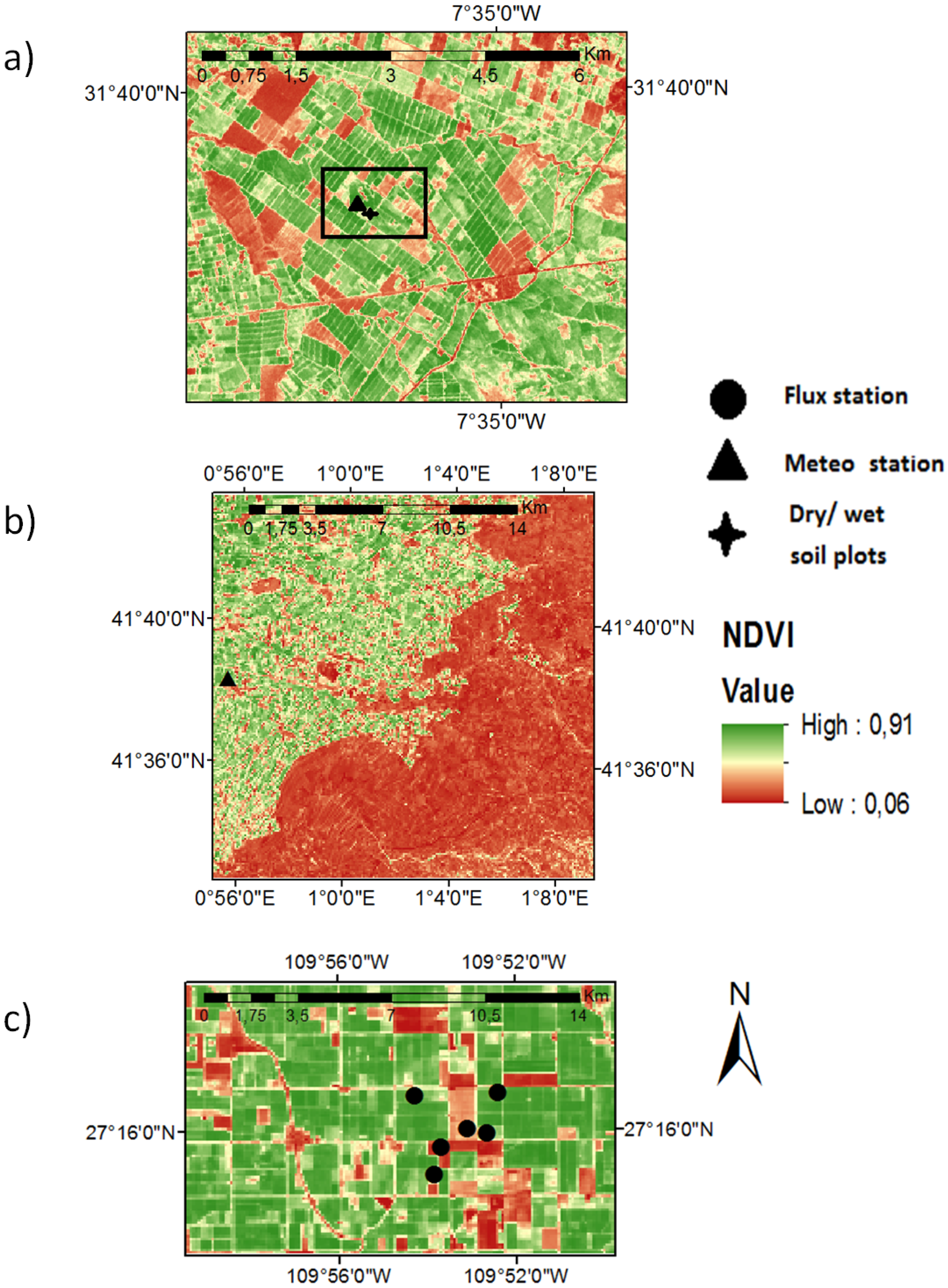
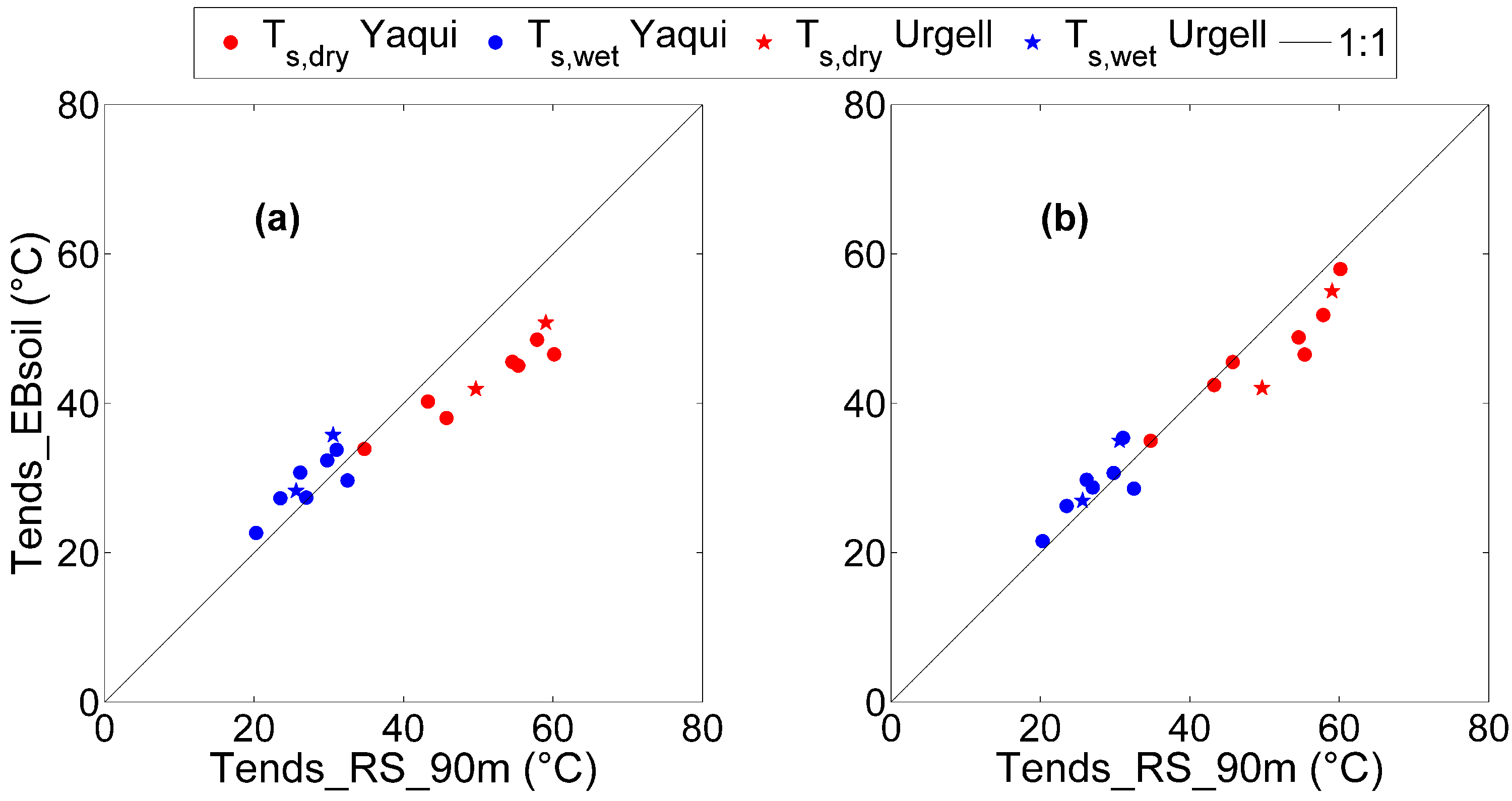
In this section, the soil Tends simulated by the soil energy balance model (Tends_EBsoil) using the RI or the MO formulation are evaluated against: (1) the in situ measurements (Tends_IS) in the R3 area; and (2) the soil Tends retrieved from 90-m resolution ASTER data (Tends_RS_90m) in the Yaqui and Urgell areas. The model-derived and image-based Tends are then used separately as input to SEB-1S when applied to 90-m resolution and to 1-km resolution (aggregated) ASTER data. The impact of Tends on contextual ET estimates is finally discussed in terms of surface conditions and observation resolution.
4.2. Application to ET Estimation at 90-m and 1-km Resolutions
One key advantage of model-derived Tends lies within the possibility to “de-contextualize” Tends submodels, meaning to extend the applicability of the so-called contextual ET models to remote sensing data at multiple spatial resolutions and to regions less heterogeneous than irrigated areas. In this study, the performance of the Tends algorithms is assessed by applying SEB-1S to both 90-m resolution and 1-km resolution data, using the model-derived or image-based Tends as input. The issue of the scale mismatch between remotely-sensed and ground-based ET estimates [
12] is addressed by the following stepwise approach: 90-m resolution SEB-1S ET is evaluated with eddy covariance measurements, and the 1-km resolution SEB-1S ET is compared to the 90-m SEB-1S ET aggregated at 1-km resolution.
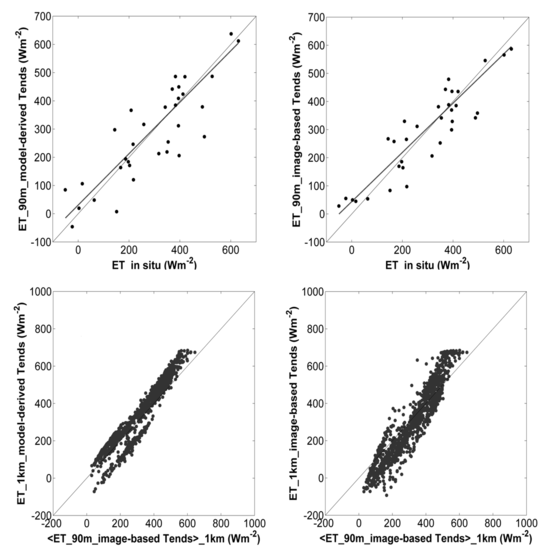
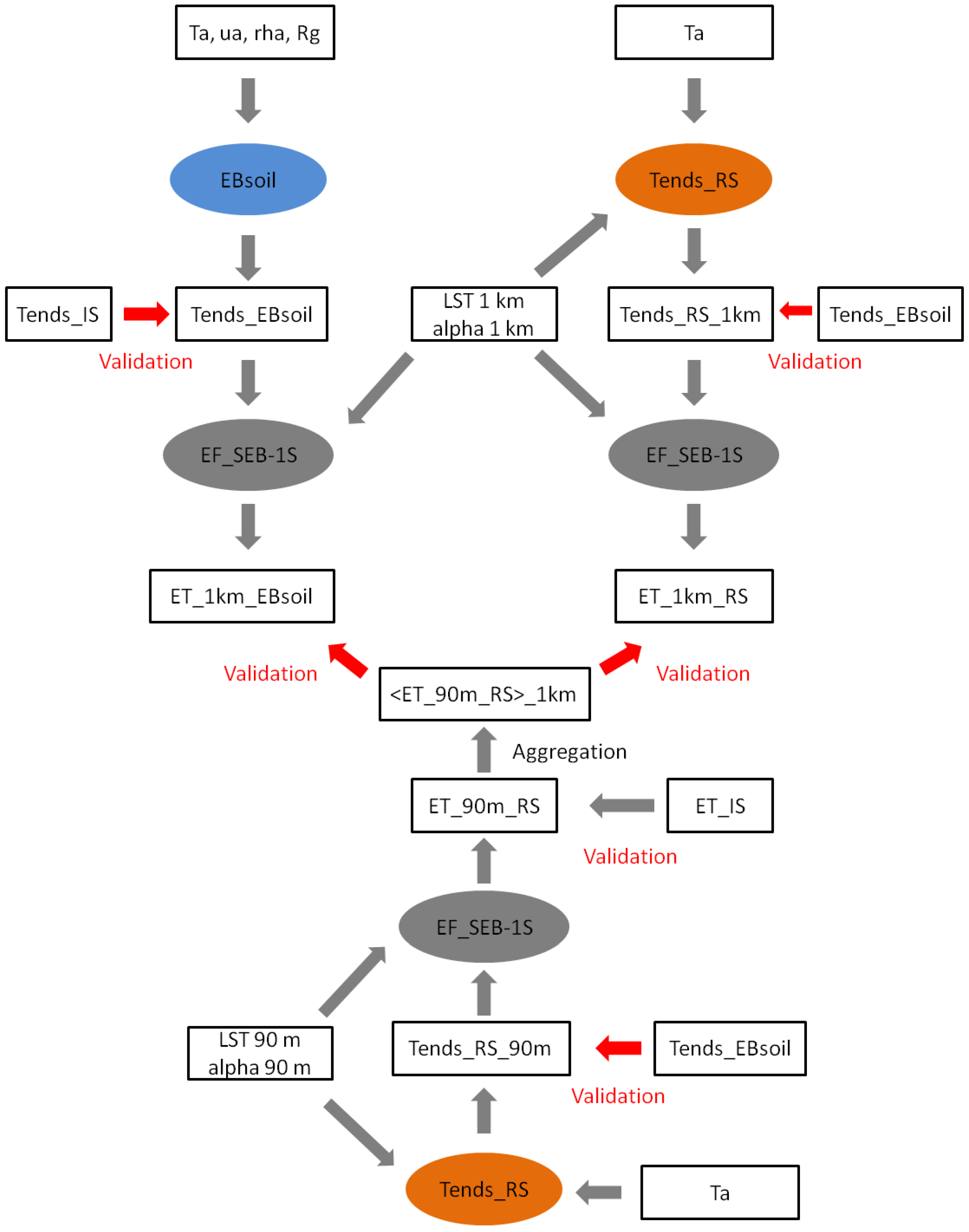
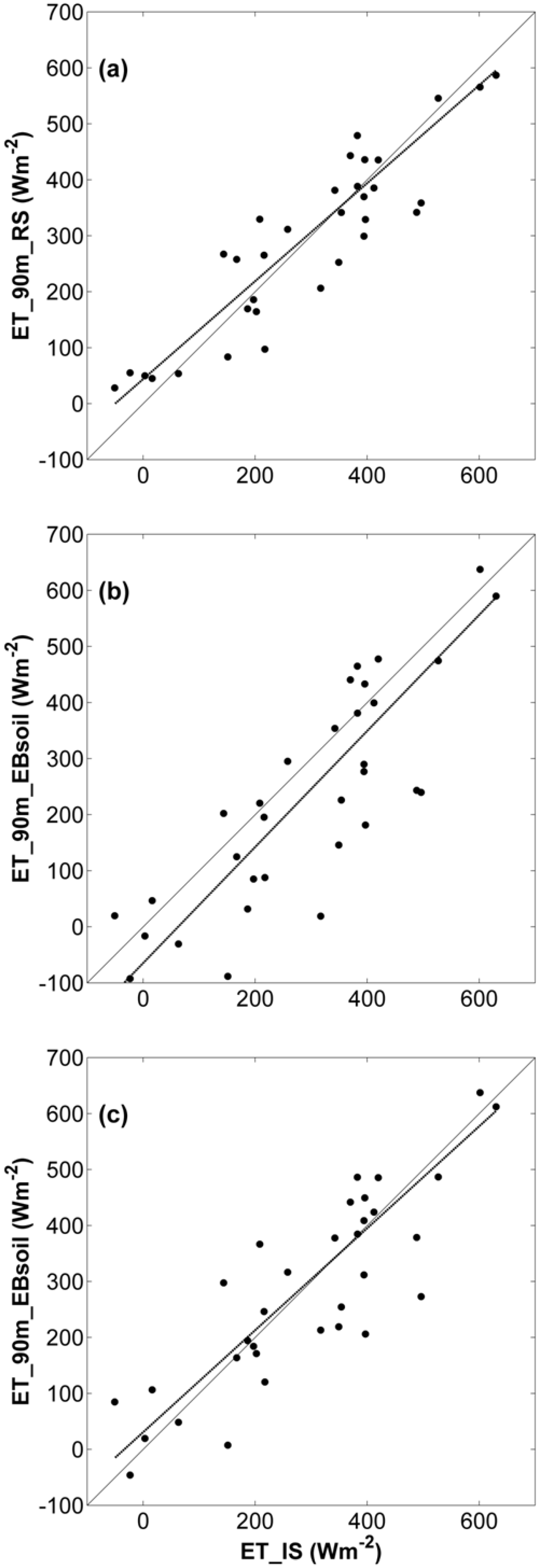
Figure 11 plots the ET simulated by SEB-1S at 90-m resolution
versus the ground-based observations of the six stations of the Yaqui experiment. SEB-1S ET estimates are obtained using the available energy (
) observed by the flux stations and either the model-derived (RI or MO
formulation) or the image-based Tends as input. The differences between the three simulation results (see the distribution of points in
Figure 11) indicate that ET is greatly influenced by EF, which strongly depends on Tends. Moreover, the
modeling approach for computing Tends has a significant impact on ET estimates. The RMSD between modeled and ground-based ET is 65, 82 and 120 W·m
for Tends_RS_90m, Tends_EBsoil with the MO
formulation and Tends_EBsoil with the RI
formulation, respectively. Tends_RS_90m-based ET estimates are in good agreement with
in situ measurements, especially given the wide observation range of ET (0–700 W·m
) [
14]. The comparison between SEB-1S and
in situ ET is also undertaken using the available energy (
) modeled by SEB-1S. In this case, the RMSD between modeled and ground-based ET is 85, 106 and 130 W·m
for Tends_RS_90m, Tends_EBsoil with the MO
formulation and Tends_EBsoil with the RI
formulation, respectively. The RMSD (65–85 W·m
) of ET obtained when using image-based Tends as input is still in the range reported by the published literature [
58,
59,
60,
61]. In the case of the Yaqui experiment, RMSD values tend to be high, because most components of the energy budget are often large in semi-arid lands at low latitudes. In addition, a fairly strong bias is present on net radiation, which tends to worsen ET estimations [
30]. Note that the significant difference in RMSD when using image-based
versus model-derived Tends as input to SEB-1S could be attributed to uncertainties in the vegetation Tends (simply derived from soil Tends and air temperature). Nonetheless, the MO
still provides acceptable ET estimates at 90-m resolution.
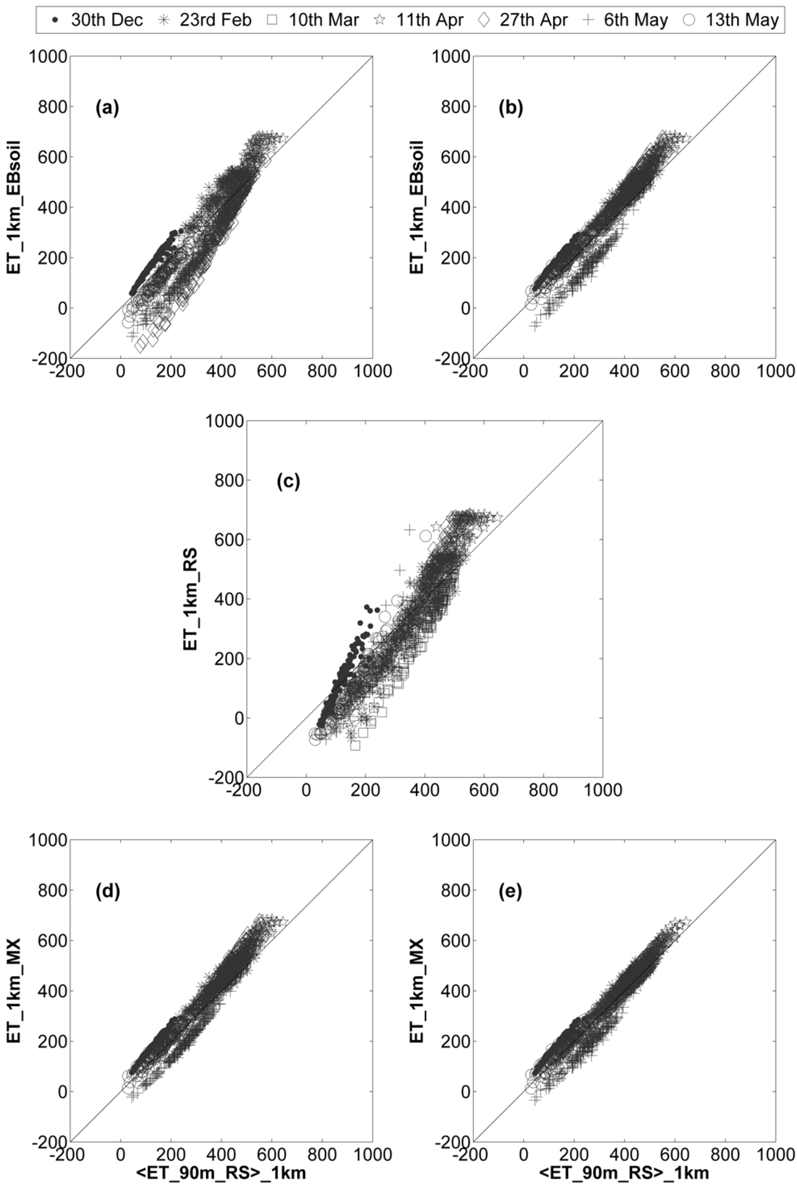
Figure 12 plots the ET simulated by SEB-1S at 1-km resolution (from aggregated ASTER data)
versus the 1-km resolution ET chosen as a reference over the Yaqui area, on all seven ASTER overpass days. Given the good results obtained with Tends_RS_90m in terms of 90-m resolution ET estimates, the reference dataset for evaluating the 1-km resolution ET models is obtained by aggregating the 90-m resolution Tends_RS_90m-forced SEB-1S ET at 1-km resolution. The Tends used as input to SEB-1S are either modeled using Tends_EBsoil with the RI or MO
formulation, or retrieved from (1-km resolution) remote sensing data using Tends_RS_1km. Statistical results, including RMSD, bias, slope of the linear regression and correlation coefficient, between simulated, and reference ET is reported in
Table 4, for each Tends algorithm and for each observation day separately. The MO formulation yet again gives the best results, with a mean RMSD of 56 W·m
compared to 77 W·m
for the RI formulation. The mean RMSD obtained when using Tends_RS_1km is close to that obtained when using the RI-derived Tends, which is 78 W·m
. However, the lowest mean bias (15 W·m
) in ET is obtained for Tends_RS_1km compared to 23 W·m
and 27 W·m
for Tends_EBsoil with the MO and RI formulations, respectively. The mean correlation coefficient is increased from 0.95 for Tends_RS_1km up to 0.98 for both Tends_EBsoil algorithms.
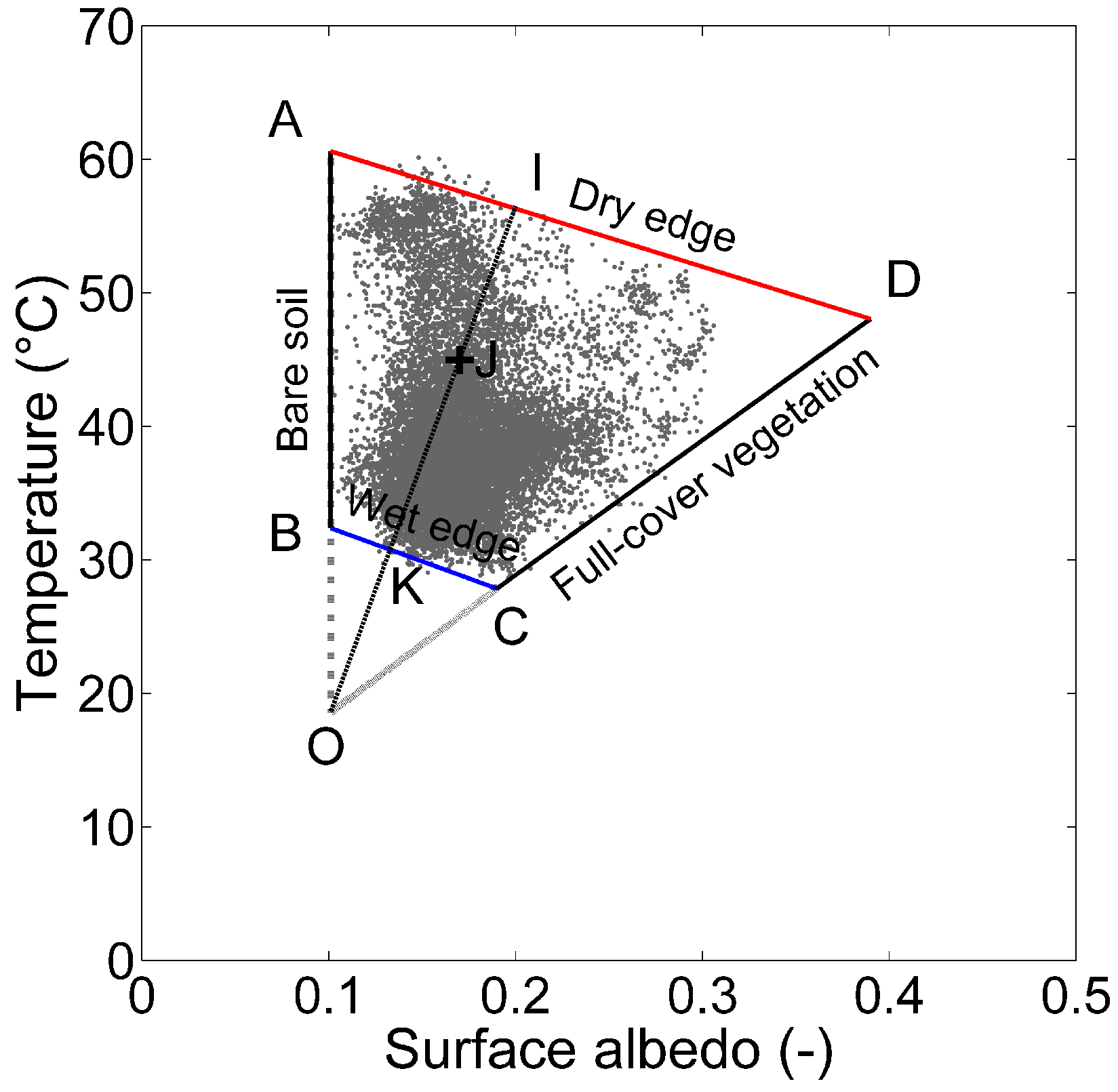
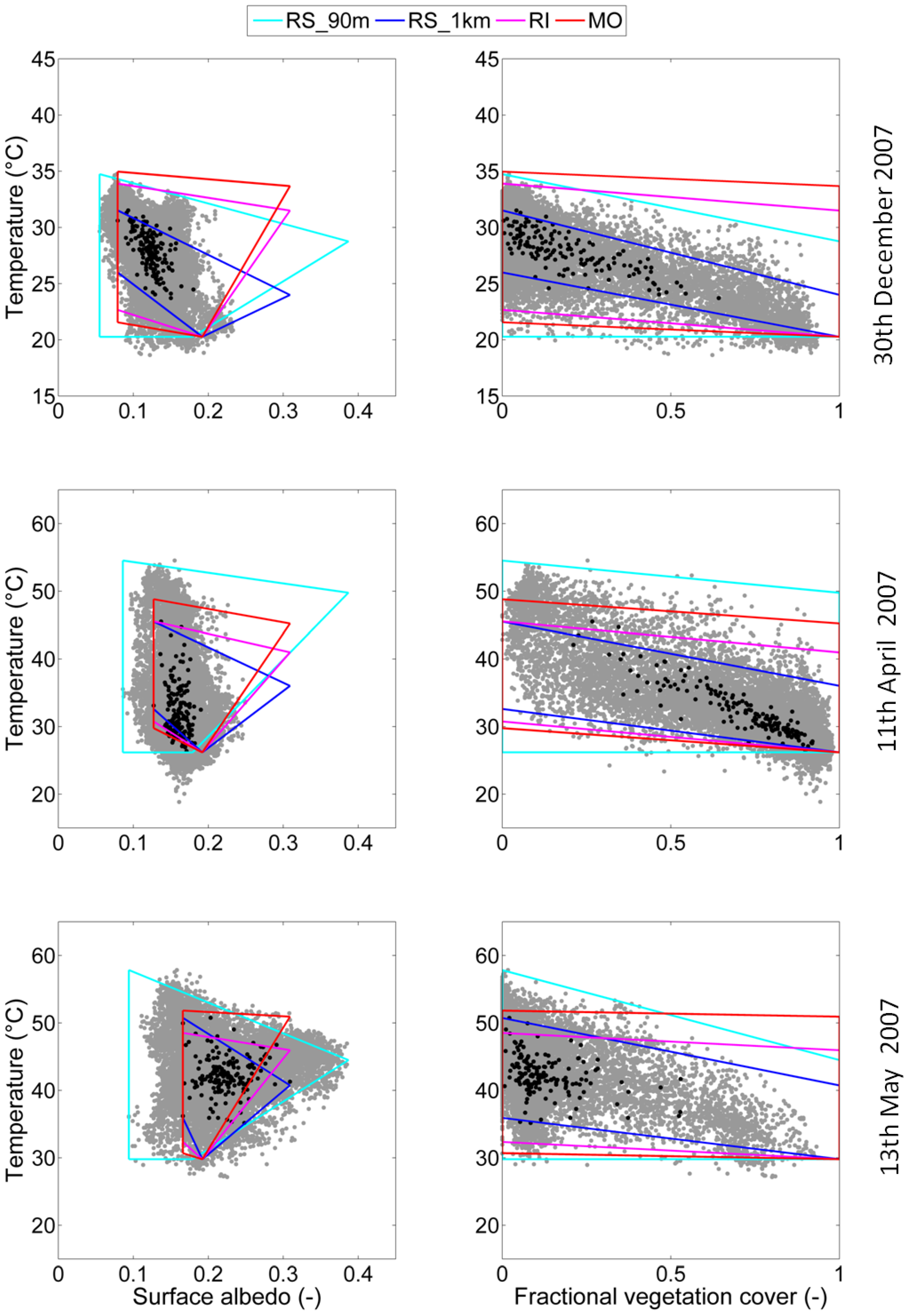
Figure 10.
The LST − α and LST − fvg spaces corresponding to 1-km resolution data (black dots) and 90-m resolution data (grey dots) are overlaid with the polygons built using Tends_RS_1km (blue), Tends_RS_90m (light blue) and the Tends_EBsoil for the RI (magenta) and MO (red) aerodynamic resistance. Results are shown over the Yaqui area (30 December, 11 April and 13 May, respectively).
Figure 11.
The ET simulated at 90-m resolution is plotted against station measurements for data over the Yaqui region. The Tends used as input to the EF_SEB-1S model consist of (a) the Tends retrieved from 90-m resolution data, (b) the Tends simulated by EBsoil with the RI and (c) MO aerodynamic resistance.
Figure 12.
The ET simulated at 1-km resolution is plotted against the 90-m resolution simulated ET, aggregated at 1-km resolution, for data over the Yaqui region, on the seven ASTER overpass dates separately. The Tends used as input to the EF_SEB-1S model consist of (a) the Tends simulated by EBsoil with the RI and (b) MO aerodynamic resistance, (c) the Tends retrieved from 1-km resolution data, (d) the Tends simulated with the mixed modeling approach using ends_1km and (e) the Tends simulated with the mixed modeling approach using ends_90m.
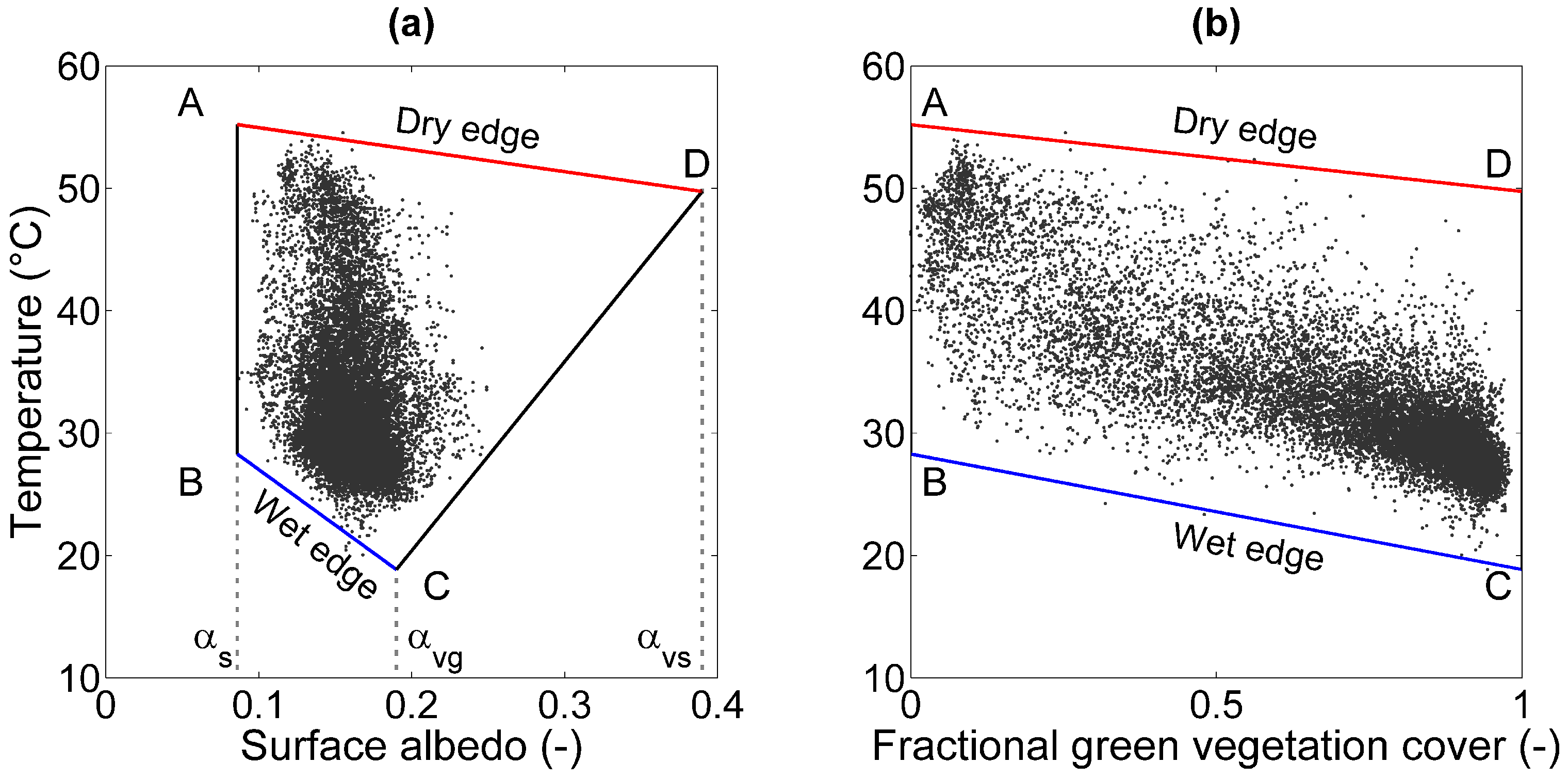
Table 4.
Root mean square difference (RMSD), bias, correlation coefficient (R) and slope of the linear regression between the ET simulated at 1-km resolution and the 90-m resolution simulated ET aggregated at 1-km resolution, for data over the Yaqui region, on the seven ASTER overpass dates separately. The Tends used as input to EF_SEB-1S consist of Tends simulated by EBsoil with the RI and MO aerodynamic resistance and the Tends retrieved from 1-km resolution data (RS).
| Date | RMSD (W·m) | Bias (W·m) | R (-) | Slope (-) |
|---|
| RI | MO | RS | RI | MO | RS | RI | MO | RS | RI | MO | RS |
|---|
| 30th Dec | 48 | 55 | 47 | 46 | 54 | 5.3 | 0.98 | 0.98 | 0.96 | 1.3 | 1.2 | 2.0 |
| 23 February | 64 | 58 | 78 | 57 | 55 | 2.0 | 0.94 | 0.96 | 0.94 | 1.1 | 0.98 | 1.7 |
| 10 March | 61 | 36 | 99 | −46 | 31 | −73 | 0.99 | 0.97 | 0.97 | 1.5 | 1.1 | 1.8 |
| 11 April | 71 | 57 | 91 | 24 | 37 | 41 | 0.97 | 0.98 | 0.96 | 1.6 | 1.4 | 1.7 |
| 27 April | 122 | 63 | 79 | −102 | 57 | 24 | 0.99 | 0.99 | 0.98 | 1.6 | 1.2 | 1.7 |
| 6 May | 127 | 95 | 82 | −126 | −93 | −52 | 0.98 | 0.98 | 0.93 | 1.2 | 1.1 | 1.6 |
| 13 May | 42 | 28 | 67 | −38 | 23 | −53 | 0.98 | 0.97 | 0.95 | 1.2 | 1.0 | 1.4 |
| All (mean) | 77 | 56 | 78 | −27 | 23 | −15 | 0.98 | 0.98 | 0.95 | 1.4 | 1.1 | 1.7 |
| All (σ) | 34 | 21 | 17 | 72 | 53 | 44 | 0.01 | 0.01 | 0.01 | 0.22 | 0.12 | 0.19 |
At 1-km resolution, the Tends_EBsoil algorithm with MO formulation improves ET predictions. However, the presence of a significant bias can be observed on the ET estimates computed using the MO-derived Tends, on 6 May. In fact, Tends_EBsoil are computed independently of the LST dataset and, thus, can lead to the polygon not being centered on the cluster points in the and spaces. This can introduce a bias in model-derived Tends and, as a result, in EF/ET. In contrast, the polygon obtained from Tends_RS_1km is centered on the cluster points, because the computation of Tends is made using the observed data points. Overall, the ET estimates derived from Tends_RS_1km have a low bias. However, the mean slope of the linear regression between modeled and reference ET is estimated as 1.7. This is due to the fact that Tends_RS_1km overestimates the wet edge and underestimates the dry edge, which translates into the polygon boundaries being too close to the point cluster. The data points are thus closer to the boundaries at 1-km resolution than at 90-m resolution, influencing the range of variability and leading to slopes significantly larger than one.
SEB-1S, as a contextual model, performs well, provided that the extreme conditions associated with fully dry and wet soil/vegetation components are encountered in the same image. Many studies have documented the sensitivity of contextual models to the wet and dry edges. For instance, Long
et al. [
19] indicated that SEBAL shows great sensitivity to extreme soil Tends, which implies that the extreme conditions play a significant role in the estimation of ET. The dry and wet edges impact the ET estimates in a similar manner: increasing Tends for the wet/dry extremes tend to increase ET based on energy conservation. Yet the distance between the observed dry and wet edges depends the range of EF, which is linked to the growth stage of vegetation and to the spatial representativeness of the study area [
8]. It also depends on the domain size. The impact of the domain size on ET estimates can reach 50–80 W·m
[
19]. When applied to moderate or low spatial resolution images, contextual models could fail to discriminate extreme soil wetness conditions and, hence, to detect EF, especially for relatively small study sites [
20]. Conversely, deriving the physical boundaries independently of remote sensing data could help improve ET estimates, especially by reducing the underestimation and overestimation of the dry and wet edge, respectively. The theoretical approach developed herein, based on a simple soil energy balance model and the MO
formulation, is well adapted for large-scale applications using moderate to low resolution data.
4.3. A Mixed Modeling Remote Sensing Approach for Improved Tends and ET estimates
As the Tends_EBsoil with the MO formulation and the Tends_RS_1km provide complementary results in terms of bias and slope of the linear regression between simulated and reference ET, a mixed modeling approach is proposed for
. The new formulation considers
as the maximum between the two estimates:
Furthermore, a new constraint concerning the albedo endmembers is applied. It consists of using either the 1-km resolution α endmembers (αends_1km) or the 90-m resolution α endmembers (αends_90m) in the estimation of Tends_RS_1km. A comparison between the 1-km resolution mixed-modeled and reference ET is also presented in
Figure 12, for the Yaqui area, on all seven ASTER overpass days, and using αends_1km (e) and αends_90m (f). Results in terms of RMSD, bias, correlation coefficient and slope of the linear regression between simulated and reference ET are reported in
Table 5, for each of the two mixed Tends formulations (MX_αends_1km and MX_αends_90m, respectively) and for the two previous configurations (MO-derived Tends_EBsoil and Tends_RS_1km, respectively). The statistical results are presented for all seven ASTER overpass dates combined. Both mixed modeling formulations significantly improve the results, with RMSD values of 43 W·m
and 52 W·m
(for MX_αends_90m and MX_αends_1km, respectively), as compared to 59 W·m
and 79 W·m
(for the MO_1km and RS_1km formulation, respectively).
Table 5.
Root mean square difference (RMSD), bias, correlation coefficient (R) and slope of the linear regression between the ET simulated at 1-km resolution and the 90-m resolution simulated ET aggregated at 1-km resolution, for data over the Yaqui region, on all of the seven ASTER overpass dates combined. The Tends used as input to EF_SEB-1S consist of Tends simulated by EBsoil with the MO aerodynamic resistance, retrieved from 1-km resolution data (RS), simulated with the mixed modeling approach using αends_1km (MX_αends_1km) and with αends_90m (MX_αends_90m).
| Configuration | RMSD (W·m) | Bias (W·m) | R (-) | Slope (-) |
|---|
| MO | 59 | 23 | 0.95 | 1.1 |
| RS | 79 | −15 | 0.93 | 1.3 |
| MX_αends_1km | 52 | 25 | 0.96 | 1.1 |
| MX_αends_90m | 43 | 9.3 | 0.96 | 1.0 |
As expected, when using the αends_90m as input to the Tends_RS_1km, the computed boundaries are much closer to the boundaries estimated at 90-m resolution. This results in the lowest bias obtained between the mixed-modeled ET at 1-km resolution (using MX_αends_90m derived Tends) and the 1-km resolution reference ET. Nevertheless, the improvement provided by the αends_90m configuration is relatively small, so that the MX_αends_1km strategy seems to be a good compromise in terms of ET accuracy and data availability. Especially the MX_αends_1km does not require high (90 m) resolution remote sensing data for calibrating αends.


 ,
, 


