Flood Mapping Based on Multiple Endmember Spectral Mixture Analysis and Random Forest Classifier—The Case of Yuyao, China

Abstract

Remote sensing is recognized as a valuable tool for flood mapping due to its synoptic view and continuous coverage of the flooding event. This paper proposed a hybrid approach based on multiple endmember spectral analysis (MESMA) and Random Forest classifier to extract inundated areas in Yuyao City in China using medium resolution optical imagery. MESMA was adopted to tackle the mixing pixel problem induced by medium resolution data. Specifically, 35 optimal endmembers were selected to construct a total of 3111 models in the MESMA procedure to derive accurate fraction information. A multi-dimensional feature space was constructed including the normalized difference water index (NDWI), topographical parameters of height, slope, and aspect together with the fraction maps. A Random Forest classifier consisting of 200 decision trees was adopted to classify the post-flood image based on the above multi-features. Experimental results indicated that the proposed method can extract the inundated areas precisely with a classification accuracy of 94% and a Kappa index of 0.88. The inclusion of fraction information can help improve the mapping accuracy with an increase of 2.5%. Moreover, the proposed method also outperformed the maximum likelihood classifier and the NDWI thresholding method. This research provided a useful reference for flood mapping using medium resolution optical remote sensing imagery.

1. Introduction

Flooding is among one of the most destructive disasters which results in tremendous economic and human losses worldwide [1,2,3,4]. It is of great significance to map accurately the extent of inundated areas and the land cover types under water [4,5], which can assist in flood monitoring, relief works planning and damage assessment.

Due to its synoptic view and continuous coverage of flooding events, remote sensing has been recognized as a powerful and effective tool to provide inundation maps in near real time according to many researches [1,2,3,4,5,6,7,8,9,10,11]. Generally, remotely sensed data used for flood monitoring are mainly collected from radar and optical satellites. The advantage of radar remote sensing is that it enables data acquisition regardless of weather conditions and time of day [7]. Space-borne sensors such as Synthetic Aperture Radar (SAR) [8] are capable of penetrating the cloud, and can provide views of the extent of inundation even when thick clouds exist above the disaster-stricken areas [1,2,6,7,8]. Brivio et al. [9] utilized visual interpretation and thresholding algorithms for multi-temporal ERS-1 (European Remote Sensing satellite) SAR data in the determination of inundated areas at the peak of the flood. Results showed that only 20% of the flooded areas were determined due to the time delay between the flood peak and the satellite overpass [9]. To tackle this limitation, Brivio et al. [9] proposed a new procedure with the synthetic use of SAR data and digital topographic data from a Geographical Information System (GIS) technique and a high proportion, 96.7%, of the flooded areas was detected [9].

Although optical sensors are unable to penetrate thick clouds which is a major drawback in flood monitoring, the images acquired under cloud free conditions can still be utilized to extract flooded areas with high accuracy [10,11,12]. Besides, optical remote sensing can provide true color images which are much easier for visual interpretation than radar data. Widely used optical remote sensing data are mainly from Landsat series, i.e., Thematic Mapper (TM), Enhanced Thematic Mapper Plus (ETM+), SPOT (Systeme Probatoire d’Observation de la Terre) series (i.e., SPOT-4, SPOT-5), and Ikonos due to their ideal combination of spatial and temporal resolutions, easy access, and ease in data processing and analysis [4]. Wang et al. [10] used medium resolution (30 m) TM images to delineate the maximum flood event caused by Hurricane Floyd in North Carolina. Animi [11] proposed a model based on Artificial Neural Network to generate a floodplain map using high-resolution (1 m) Ikonos imagery and digital elevation model (DEM). Gianinetto et al. [12] utilized multisensor data (TM and SPOT-4) to map Hurricane Katrina’s widespread destruction in New Orleans and adopted a change detection method to extract the land cover types under water. Above all, optical remote sensing can also play an important role in flood mapping given cloud free conditions.

Nevertheless, mixed pixels are common in medium spatial resolution data such as TM and ETM+, and such pixels have been recognized as a problem for remote sensing applications [13,14,15,16,17,18,19,20]. In terms of flood monitoring using medium resolution data, flooded and non-flooded features may co-exist within one pixel, resulting in the challenge to extract these small and fragmented flooded patches especially under complex urban landscapes. To deal with the mixed pixel problem, several approaches such as linear spectral mixture analysis (LSMA) [13], fuzzy-set possibilities [14], and Bayesian possibilities [15] have been developed to partition the proportions of each pixel between classes. Among these methods, LSMA appears to be the most promising and has been widely used to extract sub-pixel information with physical meaning [13,16,17,18,19]. LSMA assumes that the reflectance of each pixel can be modeled as a linear combination of a few spectrally pure land cover components, known as endmembers [13]. The aim of LSMA is to decompose a mixed pixel into the spectra of endmembers and estimate the fractional abundance of each endmember within a pixel. However, LSMA uses an invariant set of endmembers to model the entire landscape while the spectrum of each endmember is assumed to be constant across the image scene [20,21,22,23]. It neglects the fact that the same material may have different spectral curves, which cannot account for within-class spectral variability. As an extension of LSMA, multiple endmember spectral mixture analysis (MESMA) allows the type and number of endmembers to vary for each pixel, which takes into account the spectral and spatial variability of the real complex landscapes [20,21,22,23,24,25,26,27]. MESMA has been used in remote sensing fields especially in urban vegetation mapping [20,21,22,23,24,25,26,27], but to our knowledge, it has been rarely used in flood monitoring. Thus, this study aims to justify the performance of MESMA in extracting flooded areas from medium resolution remote sensing data.

Given the fact that most LSMA and MESMA applications have focused on the extraction of fractional information rather than thematic land cover types [21,22,23,24,25,26,27], this study attempted to introduce an image classifier, Random Forest (RF) [28], to classify the fraction maps generated from MESMA into different land cover categories. In general, Random Forest classifier has several advantages over other classification methods [29,30,31,32,33,34,35,36,37,38]. It is easy to parameterize, it is non-sensitive to over-fitting and is good at dealing with outliers in the training data [29]. When compared to statistical methods such as the maximum likelihood classifier (MLC), Random Forest requires no assumptions of data distribution [29], which can improve the classification performance. When compared to other machine learning methods such as support vector machine (SVM), RF has the advantage of easier parameterization and better generalization capability [30]. The successful use of SVM depends on several experiments to search for the optimal combination of kernel function type, punishment coefficient, and the kernel parameter Gamma [30]. However, the parameterization of SVM can be time consuming and cannot match that of RF. Meanwhile, RF has shown similar or even higher classification accuracy than SVM according to several studies [29,30]. RF has been widely used in remote sensing fields due to the above advantages. Rodriguez-Galiano et al. [32] utilized Random Forest for the Mediterranean land cover classification using multi-seasonal imagery and multi-seasonal texture, and the results indicated a high Kappa index of 0.92. Feng et al. [29] adopted Random Forest and texture analysis for urban vegetation mapping using high resolution UAV images and the results also showed a high classification accuracy of 90.6%. However, the usage of Random Forest in flood mapping has not been well documented and we are motivated to justify its performance in this study.

Overall, the main objective of this study is to propose a hybrid method based on MESMA and RF classifier for flood mapping using medium resolution optical satellite data. Specifically, this paper aims to (i) extend the application of MESMA to the field of flood mapping and verify its performance; (ii) justify whether Random Forest classifier can show good performance in flood mapping; (iii) discuss the merits and demerits of the proposed method based on the comparison with other state of art studies.

2. Study Area and Datasets

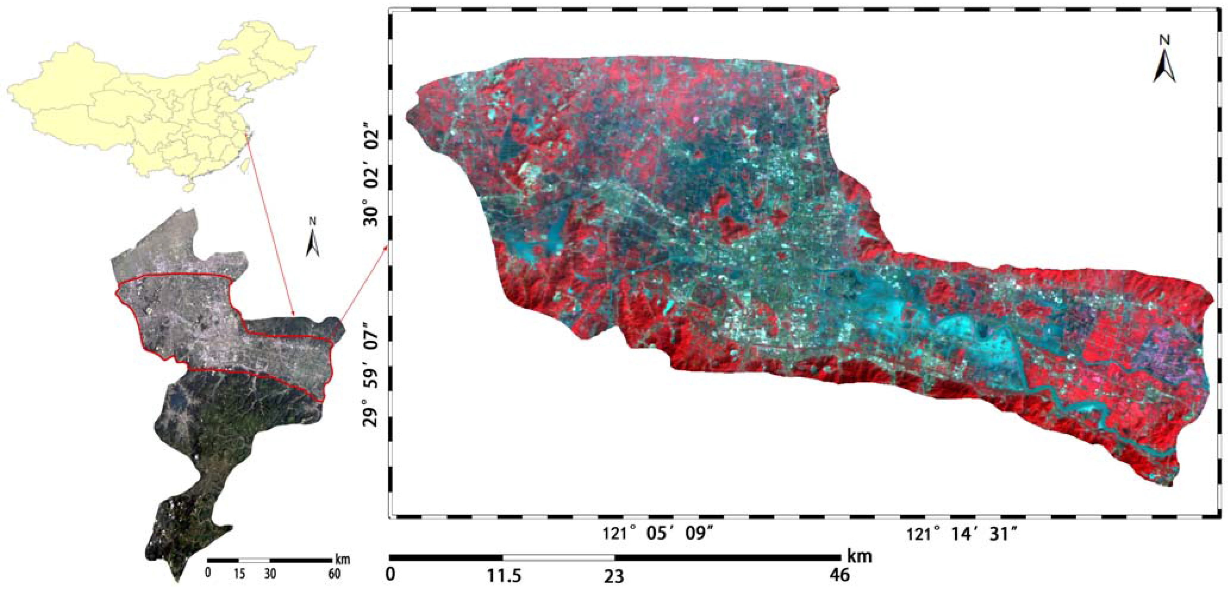
The study area is Yuyao City in Zhejiang Province in eastern China (Figure 1), which is located at the south shore of Hangzhou Bay whose coordinates are 29°–30°N, 120°–121°E. Yuyao City is located in a relatively open and flat plain while the Yuyao River flows through the middle of the whole city from west to east. The study region has a total area of 521.2 km² with an elevation range of 1 to 331 m and a slope range of 0° to 39.4°. The main land cover types include woodland (e.g., broad-leaved forest and coniferous forest), cropland (e.g., paddy rice, oilseed rape, leaf mustard), built up area (e.g., urban and suburban regions), bare soil (e.g., non-vegetated bare ground) and water (e.g., rivers, lakes, and reservoirs). Besides, the study area has an annual temperature of 16.2 °C and an average annual precipitation of 1547 mm. There is a typhoon season between May and October with an average precipitation of 5.5 mm/day in the last 60 years. Influenced by Typhoon Fitow, Yuyao experienced extreme precipitation on 7 October 2013, which led to the most serious floods in the last 60 years [30]. Typhoon Fitow brought about an accumulated rainfall of 496.4 mm in three days and the mean precipitation is about 165.5 mm/day. Most downtown areas were inundated for more than 5 days while about 833 thousand people were impacted by the disaster and the direct economic losses were more than 69.61 billion RMB (about 11.33 billion USD).

Figure 1. Study area. Red-Green-Blue composition: near-infrared, red and green bands of the multispectral charge coupled device camera (HJ-CCD) after the flood.

Figure 1. Study area. Red-Green-Blue composition: near-infrared, red and green bands of the multispectral charge coupled device camera (HJ-CCD) after the flood.

Remote sensing data used in this study were acquired by HJ-1B satellite of China on 11 October 2013. HJ-1B belongs to a small satellite constellation (HJ-1A/1B), was launched in September 2008 and is targeted for rapid mapping and monitoring of natural hazards and disasters [39]. Sensors on board HJ-1B consist of a multispectral charge coupled device camera (HJ-CCD) and an infrared camera (HJ-IRS) which have similar wavelengths to that of Landsat TM. The revisit time is four days which can meet the requirements of dynamically monitoring the flood events. The basic parameters of HJ-1B data can be viewed in Table 1.

Table 1. Parameters of HJ-1B data.

Sensor	Band	Wavelength/μm	Spatial Resolution/m	Image Breadth/km
CCD	1	0.43–0.52	30
	2	0.52–0.60	30	360
	3	0.63–0.69	30
	4	0.76–0.90	30
IRS	5	0.75–1.10	150
	6	1.55–1.75	150	720
	7	3.50–3.90	150
	8	10.5–12.5	300

Table 1. Parameters of HJ-1B data.

Sensor	Band	Wavelength/μm	Spatial Resolution/m	Image Breadth/km
CCD	1	0.43–0.52	30
	2	0.52–0.60	30	360
	3	0.63–0.69	30
	4	0.76–0.90	30
IRS	5	0.75–1.10	150
	6	1.55–1.75	150	720
	7	3.50–3.90	150
	8	10.5–12.5	300

Since Band-4 and Band-5 have similar wavelengths, we only utilized Band-4 in the analysis due to its higher spatial resolution. Besides, the data quality of Band-7 is quite low due to severe stripe noises and Band-8 belongs to a thermal infrared band; they were discarded in the following research. Thus, we only focused on the visible, near-infrared and short wave infrared wavelengths and Band-1–4 and Band-6 were selected for further analysis.

3. Method

3.1. Workflow

The workflow of this study is depicted in Figure 2 which comprises the following steps: image preprocessing, spectral unmixing using MESMA, image classification via Random Forest, and accuracy assessment. First, images acquired by both HJ-CCD and HJ-IRS after the flood event were preprocessed including radiometric calibration, geometric rectification and atmospheric correction (Section 3.2). Second, MESMA was employed to decompose the multispectral images into four fraction maps consisting of water, vegetation, impervious surface, and soil (Section 3.3). Third, both the fraction maps and the five reflectance bands together with the Normalized Difference Water Index (NDWI) and topographical parameters (DEM, slope and aspect) were included for the Random Forest classifier to determine thematic land cover types after the flood (Section 3.4). Finally, accuracy assessment was done based on the confusion matrix derived from testing samples to verify the performance of the proposed approach. Meanwhile, the importance of input variables was analyzed in Section 3.5. Variable importance is similar to variable ranking, which is provided by the Random Forest classifier to identify the contribution of each variable to the classification accuracy.

Figure 2. Workflow of this study.

Figure 2. Workflow of this study.

3.2. Image Preprocessing

Image preprocessing was a prerequisite which involved radiometric calibration, geometric rectification, and atmospheric correction. Radiometric calibration was to convert the digital numbers recorded by the sensor to radiance. Because HJ-IRS data has a spatial resolution of 150 m, it needs to be resampled at 30 m in order to match HJ-CCD data before geometric correction. Nearest Neighbor was selected as the resampling method due to its capacity in preserving the original spectral characteristics. The resampled HJ-IRS data were layer-stacked with HJ-CCD data for further processing.

The calibrated and resampled multispectral images were then geometrically rectified to a standard Landsat-8 Operational Land Imager (OLI) image, which had already been geo-corrected with a topographic map with a scale of 1:50000. The resulting root mean square error (RMSE) of the rectified image was less than 0.2 pixels which showed good accuracy.

As for atmospheric correction, by-band 6S model [40] was adopted to retrieve remote sensing reflectance from HJ-1B multispectral data. A Mid-Latitude Summer atmospheric model was used while the aerosol type was set to be continental. Other parameters such as the altitude and wavelength of the image sensor and the imaging time can be acquired through the header files of HJ-1B data. The visibility for the 6S model was set to be 36.8 km which was obtained from the local meteorological bureau. The retrieved remote sensing reflectance was then used for MESMA to derive sub-pixel fraction maps.

3.3. Multiple Endmember Spectral Mixture Analysis

As stated above, LSMA assumes that the spectrum measured by a sensor is a linear combination of the spectra of all endmembers within the pixel [13]. The mathematical model of LSMA can be expressed as Equation (1),

$$R_i={\displaystyle \sum _{k=1}^N{f}_k{R}_{ik}+{\mathrm{\epsilon }}_i}$$

(1)

where R_i is the reflectance of band i of a pixel, k is the number of endmembers, f_k is the proportion of the kth endmember within the pixel, R_ik is the reflectance of the kth endmember within the pixel in band i, ε_i is the residual of band i which indicates the unmodeled portions of the spectrum.

However, two major drawbacks exist in the LSMA method. Firstly, the number of endmembers is invariant when modeling the entire landscape using LSMA, regardless of whether the ground components represented by the endmembers are present within the pixel [20,21,22,23]. This may result in a decreased accuracy of the fractional abundance. Secondly, each endmember has only one fixed spectrum, neglecting that the same ground component may have different spectral characteristics [21,22,23]. Hence, LSMA is unable to account for with-in class spectral separability.

To address the defects of LSMA, MESMA allows the number and type of endmembers to vary on a per pixel basis to better represent the spectral variability of the complex landscapes [20], which can increase the accuracy of the estimated fractions. To be specific, MESMA consists of endmember selection and spectral unmixing modeling which is documented in the following sections.

3.3.1. Endmember Selection

Careful selection of a high quality set of endmembers is an important step in MESMA implementation [20,21,22,23,24,25,26,27]. Spectrally “pure” endmembers can be obtained from either a spectral library (reference endmember) or the remote sensing image itself (image endmember) [16,20]. In this study, image endmembers were utilized due to the following advantages: (i) they can be easily obtained and (ii) they can represent spectra measured at the same scale as the image data [16,21,22,23]. All the image endmembers were organized into four groups in this study: water, vegetation, impervious surface, and soil. Each group consisted of several subsets to represent the spectral variations for each material, e.g., vegetation (woodland, cropland), impervious surface (white material, dark material, blue roof, red roof), water (clear water, turbid water, submerged urban and suburban area), and soil. The shade endmember which has a zero value in all bands was also included here to account for the illumination variation [21,22,23].

In order to select spectrally “pure” endmembers, the pixel purity index (PPI) image was firstly calculated based on several thousand iterations of the PPI algorithm [21,22]. A higher value in the PPI image indicated a relatively purer pixel or endmember. The PPI results were also dynamically linked in an N-dimensional visualizer together with the original multispectral images to select the candidate endmembers by searching for a set of vertices on a convex hull [21].

The selected endmembers were re-selected using the following three techniques to obtain the most appropriate ones: (i) count-based endmember selection (CoB); (ii) endmember average root mean squared error (EAR) and (iii) minimum average spectral angle (MASA) [21,22,23,41]. The optimal set of endmembers was selected iteratively by adding high CoB, low EAR or low MASA endmembers to the library and assessing the model performance using root mean square error images and a visual comparison with high resolution orthoimagery [21,22,23].

Figure 3. Spectral reflectance of endmembers including (a) water; (b) vegetation; (c) impervious surface; (d) soil.

Figure 3. Spectral reflectance of endmembers including (a) water; (b) vegetation; (c) impervious surface; (d) soil.

A total of 35 optimal endmember spectra were selected using the above method from 2500 candidates. Specifically, it included twelve spectral curves for water, ten for vegetation, eight for impervious surface and five for bare soil, which are illustrated in Figure 3. Water and impervious surface spectra showed greater variation than that of vegetation and bare soil. The variation of water spectra mainly lies in that the persistent water and the submerged regions have different spectral signatures.

The whole procedure of MESMA is available in Visualization and Image Processing for Environmental Research (VIPER) tools software [41] which was adopted in this study.

3.3.2. Spectral Unmixing Modeling

After the selection of the optimal spectra for each endmember, the combinations of all the possible endmember spectra were considered to run the MESMA procedure (Table 2). Specifically, we tested 35 two-endmember models, 446 three-endmember models and 2640 four-endmember models for each pixel. The process of running the MESMA models based on the established spectral library is as follows. Take the three-endmember models as an example. Table 2 shows that the three-endmember models consisted of six combinations, i.e., water + veg + shade, water + imp + shade, water + soil + shade, veg + imp + shade, veg + soil + shade, imp + soil + shade. Because the water category had 12 spectral curves while the vegetation category had 10 spectral curves, the combination of water + veg + shade would have a total of 120 (12 × 10 × 1) SMA models. Similarly, we could calculate model numbers of the other five combinations. Hence, the three-endmember models would consist of 446 (120 + 96 + 60 + 80 + 50 + 40) SMA models. During the modeling process, several constrains must be satisfied according to previous studies [21,22,23]: (a) the non-shade fractions should be constrained between −0.05 and 1.05; (b) the maximum allowable shade fraction should be 0.8; (c) the maximum RMSE was set to be 0.025.

Table 2. Combinations of endmember models by land cover classes.

Two-Endmember (35)	Three-Endmember (446)	Four-Endmember (2640)
water + shade	water + veg + shade	water + veg + imp + shade
veg + shade	water + imp + shade	water + veg + soil + shade
imp + shade	water + soil + shade	water + imp + soil + shade
soil + shade	veg + imp + shade	veg + imp + soil + shade
	veg + soil + shade
	imp + soil + shade

Note: veg, vegetation; imp, impervious surface.

Table 2. Combinations of endmember models by land cover classes.

Two-Endmember (35)	Three-Endmember (446)	Four-Endmember (2640)
water + shade	water + veg + shade	water + veg + imp + shade
veg + shade	water + imp + shade	water + veg + soil + shade
imp + shade	water + soil + shade	water + imp + soil + shade
soil + shade	veg + imp + shade	veg + imp + soil + shade
	veg + soil + shade
	imp + soil + shade

Note: veg, vegetation; imp, impervious surface.

How the variation of the main endmembers was handled in MESMA is as follows. As for LSMA, only a few SMA models can be established due to the limited combinations of different endmembers. However, MESMA can account for the variation by considering all the combinations of the endmember spectra in order to build the candidate SMA models [21]. Meanwhile, the SMA model with the lowest RMSE was chosen as the final output for each pixel in the MESMA procedure [21]. Pixels that cannot be modeled were left unmodeled in the output. From another perspective, the variation within each endmember was an objective existence; the MESMA method allows for the establishment of all the possible combinations of SMA models to account for the variation. The mechanism in that the SMA model with the lowest RMSE was chosen as the final output makes MESMA outperform LSMA. Besides, as shade fractions were added initially to account for illumination variation and they did not belong to the interested land cover types, we generated the shade normalized maps by dividing each land cover fraction by the sum of total non-shade fractions [22].

After the implementation of MESMA, thematic land cover types should be extracted from the fraction images. However, considering that with the simple threshold method it is difficult to discriminate different land cover types from fraction maps [21,22], a machine learning based classifier, Random Forest [28] was employed to identify the land cover types using the sub-pixel fractional information. This part of the work is documented in detail in the next section.

3.4. Random Forest Classifier

Random Forest classifier was used to classify the fraction maps derived through MESMA into thematic land cover types. This supervised classifier was chosen due to its robustness and efficiency in remote sensing applications [29,30,31,32,33,34,35,36,37,38]. Besides, Random Forest has been rarely used in flood mapping and its performance needs to be studied and verified.

Random Forest is a machine learning based method proposed by Breiman [28] in 2001. It can be viewed as an ensemble of many decision trees and can be defined as Equation (2) [28],

$$\{h(x,{\mathrm{\theta }}_k),k=1,2\dots i\dots \}$$

(2)

where h represents Random Forest, x represents input variables, and {θ_k} stands for independently identically distributed random predictor variables which are used to split each decision tree. The final response of Random Forest is determined on the output of all the decision trees involved [29].

Two steps involving random selection are used to create each decision tree. First, a bootstrap strategy [28] is utilized to randomly select only 2/3 of the training samples with replacement to build each decision tree. The remaining 1/3 of the training samples are defined as out-of-bag (OOB) data [28], which are used for inner cross-validation to evaluate the performance of Random Forest. Second, only a subset of the predictor variables is randomly selected to split each tree using the Gini index [28]. Actually, the Gini index is the most frequently used attribute selection measure for splitting each decision tree, which measures the impurity of a given attribute with respect to the rest of the classes [28]. Both of the two random selection steps result in less correlation between the decision trees and thus a higher generalization capability of the Random Forest classifier. Besides, the importance of input variables can be measured, which indicates their contributions to the classification accuracy [28,29].

The parameterization of Random Forest classifier is simple and can be carried out using the package random Forest in R language [42,43]. Only two parameters need to be specified including ntree and mty. ntree is the number of decision trees making up the whole forest. In general, the OOB error decreases with the growth of ntree and the plot of OOB error vs. ntree is always necessary to see whether the number of trees is sufficient in the grown forest [34]. mty is the number of randomly selected predictor variables. Two methods [28] are commonly used to calculate mty, i.e., one-third or square root of the number of input variables.

In this research, the four shade-normalized fraction images generated from MESMA, together with the five spectral bands were included as input for the Random Forest classifier. Besides, since the main interest of this study was with the extraction of inundated extent, an additional image of the normalized difference water index [44] was also included for image classification. In general, the Normalized Difference Spectral Indices (NDSIs) is suitable for detecting the open water surface and the inundated areas. Boschetti et al. [45] provided a useful review which summarized and compared dozens of NDSIs for detecting surface water in flooded rice fields, which also shed light on the inundated area detection. Moreover, the water related spectral indices are proposed as the combination of shortwave infrared and near infrared or visible spectral regions [45]. Due to the band positions of the HJ satellite data, we incorporated a normalized difference water index as shown in formula (3):

$$\text{NDWI}=\frac{\mathrm{\rho }(\text{Green})-\mathrm{\rho }(\text{NIR})}{\mathrm{\rho }(\text{Green})+\mathrm{\rho }(\text{NIR})}$$

(3)

where ρ(Green) and ρ(NIR) refer to the reflectance of the green band (Band-2) and near infrared band (Band-4), respectively.

Meanwhile, to improve the separability of different land cover types, the topographical parameters were also added here including DEM, slope, and aspect. The DEM, with a spatial resolution of 30 m, was derived from the Advanced Spaceborne Thermal Emission and Reflection Radiometer Global Digital Elevation Model (ASTER GDEM) products [11].

According to visual interpretation through high resolution unmanned aerial vehicle photos [30], five classes were chosen for the entire image as follows, water, built-up, woodland, cropland, and bare soil. The selection procedure of training and testing samples is of great significance in supervised image classification. According to previous studies [29,46], there are several selection strategies including single pixel selection, similar contiguous pixels through seeding, and polygon-block selection. In this study, a polygon-block sampling procedure was utilized according to Chen et al. [46]. All the training and sampling were selected by visualizing and digitizing small polygons or blocks of pixels, and it was assumed all the pixels within each polygon belong to the same land cover category [46]. Usually there were two to six pixels in a polygon utilized in this research. Besides, all the training and testing samples were derived from the remote sensing image based on high resolution areal image, Google Earth history image and a priori knowledge. Each land cover type had 200 training points to train the Random Forest classifier in order to avoid any under- or over-estimation of the spectral patterns. The trained Random Forest was then utilized to classify the input images. Next, the non-water classes (woodland, cropland, built up area, and bare soil) were merged into the non-flooded class to simplify the problem while the flooded class was extracted by subtracting the persistent water. The “persistent water” was derived from the “water” class of the classification result of the pre-flood image (2013.09.10). Because the “real” flooded area and the persistent water were both included in the “water” class of the classification result of the flooding image (2013.10.11), the persistent water was then utilized to separate the “real” flooded areas.

3.5. Accuracy Assessment

In order to quantitatively assess the accuracy of the proposed method, the confusion matrix was calculated from the validation samples. Overall accuracy, producer accuracy, user accuracy, and the Kappa index can be derived from the confusion matrix to justify the performance of the hybrid approach.

There were only two land cover types, i.e., non-flooded class and flooded class in the accuracy assessment. Each of the non-flooded and flooded classes had 200 testing points to derive the confusion matrix. Besides, the testing points were selected independently from the training points, using the polygon-block selection procedure [46]. The spatial distribution of training and testing samples of the “water” class is depicted in Figure 4. Actually, the “point” in Figure 4 is a small polygon containing several pixels which is assumed to belong to the same land cover category. Besides, all the testing points were derived manually based on a priori knowledge and reference images, therefore, under this context, testing points can be distributed almost evenly among the whole study area through manual selection. Although it can generate some bias when compared to the statistical sampling method, the above sampling method can be feasible and acceptable in the remote sensing field [29,46].

Figure 4. Spatial distribution of training and testing points for “water” class.

Figure 4. Spatial distribution of training and testing points for “water” class.

4. Results

4.1. Fraction Maps Derived from MESMA

After the procedure of MESMA, four fraction maps including water, vegetation, impervious surface, and soil can be derived and are shown in Figure 5. Red areas represent high fractions while blue areas mean low fractions.

Figure 5. Fraction maps derived from multiple endmember spectral analysis (MESMA) including (a) water; (b) vegetation; (c) impervious surface; (d) soil.

Figure 5. Fraction maps derived from multiple endmember spectral analysis (MESMA) including (a) water; (b) vegetation; (c) impervious surface; (d) soil.

Figure 5 indicates that MESMA can generate precise fraction maps for the entire post-flood regions. The peripheral regions of the reservoir (on the left side of the image) and the Yuyao River, which also belong to the flooded areas, have a high value of water fractions (Figure 5a). The extent of Yuyao City, which manifests itself with high values in the impervious surface fraction map, is clearly depicted in Figure 5c. The high vegetation fractions are mainly located outside the city core (Figure 5b) while the soil fractions are relatively lower and scattered among the vegetated areas (Figure 5d). Above all, the fraction maps derived from MESMA shows distinct differences between each other, which can improve the between-class separability of different land cover types.

4.2. Parameterization of Random Forest

As stated in Section 3.4, two important parameters including mty (the number of randomly selected predicable variables) and ntree (the number of individual trees) should be determined. Since the input image consisted of 13 bands, i.e., five spectral bands, four fraction bands, one NDWI band and three topographical bands, thus mty was set to be 3.61, which was the square root of the number of input variables. As for ntree, the optimal value should make the OOB error of RF converge. We set it to be 200 according to our previous studies [29,30], and the plot of ntree vs. OOB error is depicted in Figure 6 to justify whether 200 trees is enough for the classifier.

Figure 6. Out-of-bag (OOB) error vs. ntree.

Figure 6. Out-of-bag (OOB) error vs. ntree.

Figure 6 depicts clearly that the OOB error has already been convergent when ntree reaches 200. Specifically, the OOB error decreases sharply from 17.4% to 3.1% while ntree increases from 1 to 15. After that, the OOB error drops slowly and begins to show convergence. Besides, Figure 6 also indicates that ntree = 50 or 100 witnessed a similar OOB error to that of ntree = 200, however, the OOB error curve showed greater fluctuations at ntree = 50 or 100 than ntree = 200. Therefore, we rendered that a number of 200 decision trees shows more robustness and ntree was then set to be 200 in the Random Forest classifier.

4.3. Flood Mapping Results

The Random Forest classifier with 200 decision trees was incorporated to classify the post-flood image containing 13 input bands into five land cover types: water, woodland, cropland, impervious surface, and bare soil. The final flood map was generated through the merging of non-water land cover types into the non-flooded class and the subtracting of persistent water from the water class (Figure 7).

Figure 7. Flooded areas generated through RF classifier.

Figure 7. Flooded areas generated through RF classifier.

As depicted in Figure 7, the red areas represent the flooded extent while the blue areas stand for the persistent water. In order to manifest the inundated areas more obviously, the original true color remote sensing image is set to be the background on which the flood mapping result is overlaid. Figure 7 also illustrates that the inundated areas show distinct spatial patterns. Large flat areas along the branches of the Yuyao River were submerged due to the overflow of the rivers. The downstream area of the reservoir which lies on the left side of the image was also inundated due to the flood discharge through the dam. Besides, vast areas of low-lying cropland, adjacent to the northwestern part of the city core, were submerged.

Moreover, land cover maps just before a flood event should be useful to help extract submerged land cover types and areas to assist disaster loss evaluation and post-disaster reconstruction. HJ-CCD and HJ-IRS images acquired on 10 September 2013 were selected to generate the land cover map before the flood, also using the proposed method in this study. Specifically, MESMA together with Random Forest classifier were utilized to derive the land cover types of the pre-flood image. First, 32 optimal spectral curves (nine for water, ten for vegetation, eight for impervious surface and five for bare soil) were selected for the MESMA model to derive the fractional information. Second, NDWI of the pre-flood image, together with DEM, slope, aspect, original spectral bands, and fractional bands were layer stacked for the Random Forest classifier with 200 decision trees. A number of 200 testing points for each land cover type were selected to calculate the confusion matrix and the result showed high performance with an overall accuracy of 91.20% and a Kappa index of 0.89, which can provide accurate and reliable data source to derive the inundated land cover types and areas. The pre-disaster land cover map is shown in Figure 8.

Figure 8. Land cover types before the flood event.

Figure 8. Land cover types before the flood event.

Figure 8 illustrates that the city core is centered in the study area while the suburban areas possess large areas of cropland and scattered villages. The woodland is mainly located on the mountains adjacent to the floodplain while the bare soil is mainly located where the forest had been cut down. The area (km²) and proportion (%) of pre-flood land cover types are listed in Table 3.

Table 3. Area and proportion of the land cover types before the flood.

Pre-Flood Land Cover Type	Area (km2)	Proportion
Woodland	76.023	14.59%
Cropland	294.823	56.56%
Built up area	136.145	26.12%
Bare soil	4.100	0.79%
Water	10.124	1.94%
Total	521.215	100.00%

Table 3. Area and proportion of the land cover types before the flood.

Pre-Flood Land Cover Type	Area (km2)	Proportion
Woodland	76.023	14.59%
Cropland	294.823	56.56%
Built up area	136.145	26.12%
Bare soil	4.100	0.79%
Water	10.124	1.94%
Total	521.215	100.00%

It can be observed that cropland was the dominant land cover type with a percentage of 56.56%, followed by built up area (26.12%) and woodland (14.59%). Water and bare soil accounted for a small proportion of 1.94% and 0.79%, respectively. The pre-disaster land cover map and the flood map were sent for a GIS analysis to compute the land cover types and areas intersected by flooding (Table 4).

Table 4. Inundated land cover types and area statistics.

Inundated Land Cover Type	Area (km2)	Proportion
Woodland	0.075	0.07%
Cropland	76.133	75.66%
Built up area	24.373	24.23%
Bare soil	0.039	0.04%
Total	100.620	100.00%

Table 4. Inundated land cover types and area statistics.

Inundated Land Cover Type	Area (km2)	Proportion
Woodland	0.075	0.07%
Cropland	76.133	75.66%
Built up area	24.373	24.23%
Bare soil	0.039	0.04%
Total	100.620	100.00%

Table 4 indicates that a total area of about 100 km² was inundated after the flood event. Among this, about 76 km² was cropland and 24 km² was built-up areas which altogether account for about 99% of all the inundated areas. There existed very little woodland and bare soil that had been submerged. Furthermore, the fact that large cropland and built-up areas were flooded indicates that great economic losses had occurred, including the reduction of agriculture yield, the stagnation of industrial production, etc.

4.4. Results of Accuracy Assessment and Variable Importance

In order to quantitatively justify the performance of the proposed method, accuracy assessment was carried out based on the confusion matrix derived from validation data (Table 5). It indicates that the proposed method can extract the inundated areas accurately with an overall accuracy of 94% and a Kappa index of 0.88. Besides, more flooded testing points were misclassified as non-flooded (17) than the situation in which non-flooded were misclassified as flooded (7), meaning that the proposed method has the tendency to underestimate the flooded areas.

Table 5. Confusion matrix for two land cover types.

Classification Results	Validation Data
	Flooded	Non-flooded	UA (%)
Flooded	183	7	96.3
Non-flooded	17	193	91.9
PA (%)	91.5	96.5%
OA (%)	94	Kappa	0.88

Notes: PA, Producer Accuracy; UA, User Accuracy; OA, Overall Accuracy.

Table 5. Confusion matrix for two land cover types.

Classification Results	Validation Data
	Flooded	Non-flooded	UA (%)
Flooded	183	7	96.3
Non-flooded	17	193	91.9
PA (%)	91.5	96.5%
OA (%)	94	Kappa	0.88

Notes: PA, Producer Accuracy; UA, User Accuracy; OA, Overall Accuracy.

It is necessary to show the accuracy assessment of the overall five land cover classes. To calculate the confusion matrix, 200 testing points were selected for each class and the following Table 6 shows the accuracy assessment results for the entire five land cover types.

Table 6. Confusion matrix for five land cover types.

Class	Validation Data
	Woodland	Cropland	Built up	Bare soil	Water	UA (%)
Woodland	158	0	0	0	0	100.00
Cropland	31	173	0	0	0	84.80
Built up	1	8	200	9	16	85.47
Bare soil	1	0	0	191	0	99.48
Water	9	19	0	0	184	86.79
PA (%)	79.00	86.50	100.00	95.50	92.00
OA (%)	90.60		Kappa	0.8825

Table 6. Confusion matrix for five land cover types.

Class	Validation Data
	Woodland	Cropland	Built up	Bare soil	Water	UA (%)
Woodland	158	0	0	0	0	100.00
Cropland	31	173	0	0	0	84.80
Built up	1	8	200	9	16	85.47
Bare soil	1	0	0	191	0	99.48
Water	9	19	0	0	184	86.79
PA (%)	79.00	86.50	100.00	95.50	92.00
OA (%)	90.60		Kappa	0.8825

Table 6 indicates that the classification errors mainly occurred between woodland and cropland, water and cropland, water and built up area. The spectral similarity between forests and crops accounts for the classification errors between woodland and cropland. Meanwhile, the errors between water (mainly flooded areas), cropland, and built up area lie in the fact that a large amount of croplands and built up areas were submerged by the flood water, which resulted in the spectral confusion that accounts for the classification errors.

Another important characteristic of Random Forest classifier is that it can provide the importance of input variables, which can be used to measure their contribution to the classification accuracy. Actually, the variable importance can play a role in feature selection in choosing the more important variables for further classification [32]. The feature selection process is significant especially when several dozens of variables are used and the amount of calculations are correspondingly heavy [32]. Therefore, it is possible to re-run the RF classifier without the less important variables to reduce the amount of calculations. However, we did not discard any input variables because the number of variables was small in this study and the amount of calculation was acceptable. The importance of all the 13 input variables is depicted in Figure 9. In general, the original reflectance bands are more important than fraction bands and topographical bands. The near-infrared band (Band-4) is the most important followed by the short wave infrared band (Band-6). This is partly because the reflectance of water is very low in those two bands, which helps to increase the difference between flooded and non-flooded regions. As for the fraction bands, the water fraction is more important and this is predictable since water fraction can help provide sub-pixel information of the flooded areas.

Figure 9. Importance of input variables.

Figure 9. Importance of input variables.

4.5. Comparison with Other Methods

To further verify the performance of the proposed method, a series of comparison experiments was carried out. First, Random Forest was utilized to classify the input image without fractions to verify whether the inclusion of fraction information can improve the classification accuracy. Next, maximum likelihood classifier (MLC) was incorporated as a benchmark to classify both the input image, with and without fraction information. Also, the same training and validating data were used during all the classification to ensure comparability. Finally, the traditional NDWI thresholding method was utilized to extract the flooded areas. A trial and error approach was employed to determine the optimal threshold of NDWI and the final threshold was set to be –0.18. The results of the above comparison experiments are listed in Table 7.

Table 7. Comparison of the classification results by different approaches.

	MESMA + RF	RF-Only	MESMA+MLC	MLC-Only	NDWI-Thresholding
OA (%)	94	91.5	92	89	82.3
Kappa index	0.88	0.83	0.84	0.78	0.65

Notes: MESMA+RF, the proposed method; RF-only, using RF to classify the input image without fraction bands; MESMA+MLC, using MLC to classify the input image with fraction bands; MLC-only, using MLC to classify the input image without fraction bands. Maximum likelihood classifier (MLC). Multiple endmember spectral analysis (MESMA). Random Forest (RF). Normalized Difference Water Index (NDWI).

Table 7. Comparison of the classification results by different approaches.

	MESMA + RF	RF-Only	MESMA+MLC	MLC-Only	NDWI-Thresholding
OA (%)	94	91.5	92	89	82.3
Kappa index	0.88	0.83	0.84	0.78	0.65

Notes: MESMA+RF, the proposed method; RF-only, using RF to classify the input image without fraction bands; MESMA+MLC, using MLC to classify the input image with fraction bands; MLC-only, using MLC to classify the input image without fraction bands. Maximum likelihood classifier (MLC). Multiple endmember spectral analysis (MESMA). Random Forest (RF). Normalized Difference Water Index (NDWI).

Table 7 indicates that the proposed method in this study yields the highest accuracy. The inclusion of fraction information increases the overall accuracy by 2.5% when comparing MESMA+RF to RF-only. Similarly, when using MLC, the overall accuracy rises by 3% after the addition of fraction bands, indicating that the inclusion of sub-pixel fractions can improve the classification accuracy regardless of the type of classifiers. Besides, RF outperformed MLC with an increase of 2% and 2.5% in classifying the images with and without fractions bands, respectively. The traditional NDWI thresholding method shows the lowest accuracy of 82.3%, indicating that it is inferior to these classification methods. Although the inclusion of MESMA based fraction images only increased the classification accuracy by 2.5% for RF classifier, this was derived from the classification results of only one study area during the flooding period. However, when considering the classification results of the pre-flood image, the inclusion of MESMA improved the accuracy by 4.7% of RF, which was higher than that of the flood image. Therefore, future studies should include more study cases to further verify the role of MESMA in the improvement of classification accuracy.

5. Discussion

Experimental results demonstrated that both the flood map and pre-flood land cover map can be derived accurately from the proposed method, which provides reliable and valuable information for flood management and hazard assessment. The advantage of the proposed method lies in the integration of MESMA and RF classifier. Specifically, due to its capability to account for the spectral and spatial variability of complex landscapes [21], the adoption of MESMA can tackle the mixed pixel problem of flood mapping when using medium resolution remote sensing data. In previous studies [20,21,22,23,24,25,26,27], MESMA was successfully utilized in several application fields, such as mapping vegetation types under complex urban environment [21], mapping burn severity in Mediterranean countries from moderate resolution satellite data [22], and mapping urban land cover types using HyMap hyperspectral data [26], etc. This study introduced MESMA into the field of flood mapping, which broadens its range of application and provides a new clue on deriving inundated areas accurately from medium resolution data. Besides, the adoption of the robust and efficient RF classifier also contributes to the high performance of this research. In previous studies of flood mapping [8], statistical classifier such as MLC was widely used. However, MLC is inferior to RF classifier according to several studies [29,30,31], therefore, we introduced RF classifier to improve the classification accuracy in the field of flood mapping.

Meanwhile, it is necessary to compare with other literature on flood mapping to further verify the performance of the proposed approach. These state of art studies include water index (WI) [44,45], linear spectral mixture analysis [47], artificial neural network (ANN) [11] and object based image analysis (OBIA) [8]. To begin with, water index (e.g., NDWI) has been widely used for the detection of open surface water and inundated areas. The advantage of the water index lies in its simplicity and practicality, which can enhance open water features and suppress built up, vegetation and soil noise at the same time [44]. Memon et al. (2012) [48] used three water indexes for delineating and mapping of surface water using MODIS (Terra) near real time images during the 2012 floods in Pakistan. The three water indexes included NDWI, Red and Short Wave Infra-Red (RSWIR) water index [49] and Green and Short Wave Infra-Red (GSWIR) water index [50]. Experimental results indicated the accuracy of NDWI, RSWIR, and GSWIR was 73.12%, 85.80%, and 81.54%, respectively, which was lower than the proposed MESMA+RF approach (94%). This was mainly due to the fact that the vegetation has relatively high reflectance in the NIR region, so the water indexes could not take water under vegetation into account [48]. Therefore, the co-existence of flooded water and vegetation within one pixel would lead to the underestimation of flooded areas when using water indexes. However, MESMA can derive the sub-pixel water information from the mixed pixels, which accounts for a higher accuracy than with the water index thresholding methods.

Juan et al. (2012) [47] utilized linear spectral mixture analysis as part of the proposed sub-pixel analysis methodology to identify flooded areas from MODIS remote sensing data. The proposed methodology was demonstrated to be effective for mapping the flood extent with an accuracy of 80% [47]. However, the proposed approach of our paper outperformed that of Juan et al. One possible reason lies in that Juan et al. only adopted the LSMA model, which used an invariant set of endmembers (water, vegetation, etc.) to model the complex flooded landscape and could not account for the within-class variance [21]. On the other hand, MESMA allowed the type and number of endmembers to vary on each pixel [22], which could yield more accurate fractional information than LSMA.

Artificial neural network was employed in Amini’s study (2010) [11] to classify the high-resolution Ikonos image to determine the inundated classes after flooding. A multi-layer perceptron neural network was chosen due to its ability to implement nonlinear decision functions and the fact that no prior conjectures needed to be made for the input data [11]. Results showed that the utilization of ANN achieved an accuracy of 70% and outperformed MLC with an accuracy increase of 15% [11]. Meanwhile, the proposed MESMA+RF method outperformed that of Amini. One possible interpretation is that ANN has the drawback of a low generalization capability due to over-fitting of the training data, which leads to the decline of performance in predicting new datasets. However, RF uses a bootstrap strategy to generate independent training samples to tackle the problem of over-fitting, which accounts for the higher accuracy when compared with ANN.

In addition, as one important method in remote sensing image classification, object based image analysis has also been applied in detecting inundated areas. Mallinis et al. (2013) [8] utilized Geographic Object-Based Image Analysis (GEOBIA) and Landsat TM data for flood area delineation. Results indicated that the proposed GEOBIA based method showed high performance and attained an overall accuracy of 92.67% in inundated-areas detection [8]. The advantage of OBIA in flood mapping is the ability to incorporate semantic knowledge in the classification process, thus restricting limitations resulting from imagery characteristics and temporal availability [8]. The RF classifier used in this paper is a pixel-based method, although it has a similar accuracy to that of OBIA, it may still cause a “salt and pepper” effect in the classification results. Therefore, future study should be focused on incorporating OBIA into the RF classifier to further increase the accuracy of flood mapping.

Although the above discussion verifies the high performance of the proposed approach of the study, there are still some limitations which can be stated as follows. First, the optical sensor’s inability to penetrate the canopies of forests can cause the underestimation of flooded areas in the woodland region. The fact that only 0.075 km² of woodland was detected as flooded in this study supported this point of view. This is in accordance with Wang’s study [10], which found that scattered “holes” or “islands” exited in the submerged forest areas. To tackle this issue, radar data should be incorporated and future study should focus on the fusion of multi-sensor (optical and radar) data to increase flood mapping accuracy. Second, the underestimation of flooded areas in the built up regions was also a problem. This is due to the fact that some submerged roads are too narrow to be detected in the medium resolution HJ data (30 m). The buildings adjacent to the submerged roads usually have a very high reflectance and will cover the signal of the flooded roads within one pixel. Although MESMA can tackle the mixed pixel problem to some degree, however, high resolution remote sensing data should be used in order to generate more accurate flood maps in built up areas such as city blocks and factories.

Meanwhile, the proposed MESMA+RF method can be extended to other remote sensing applications such as the extraction of imperious surface from medium resolution satellite data and land cover mapping using airborne hyperspectral remote sensing data.

6. Conclusions

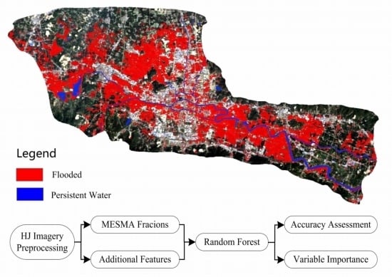
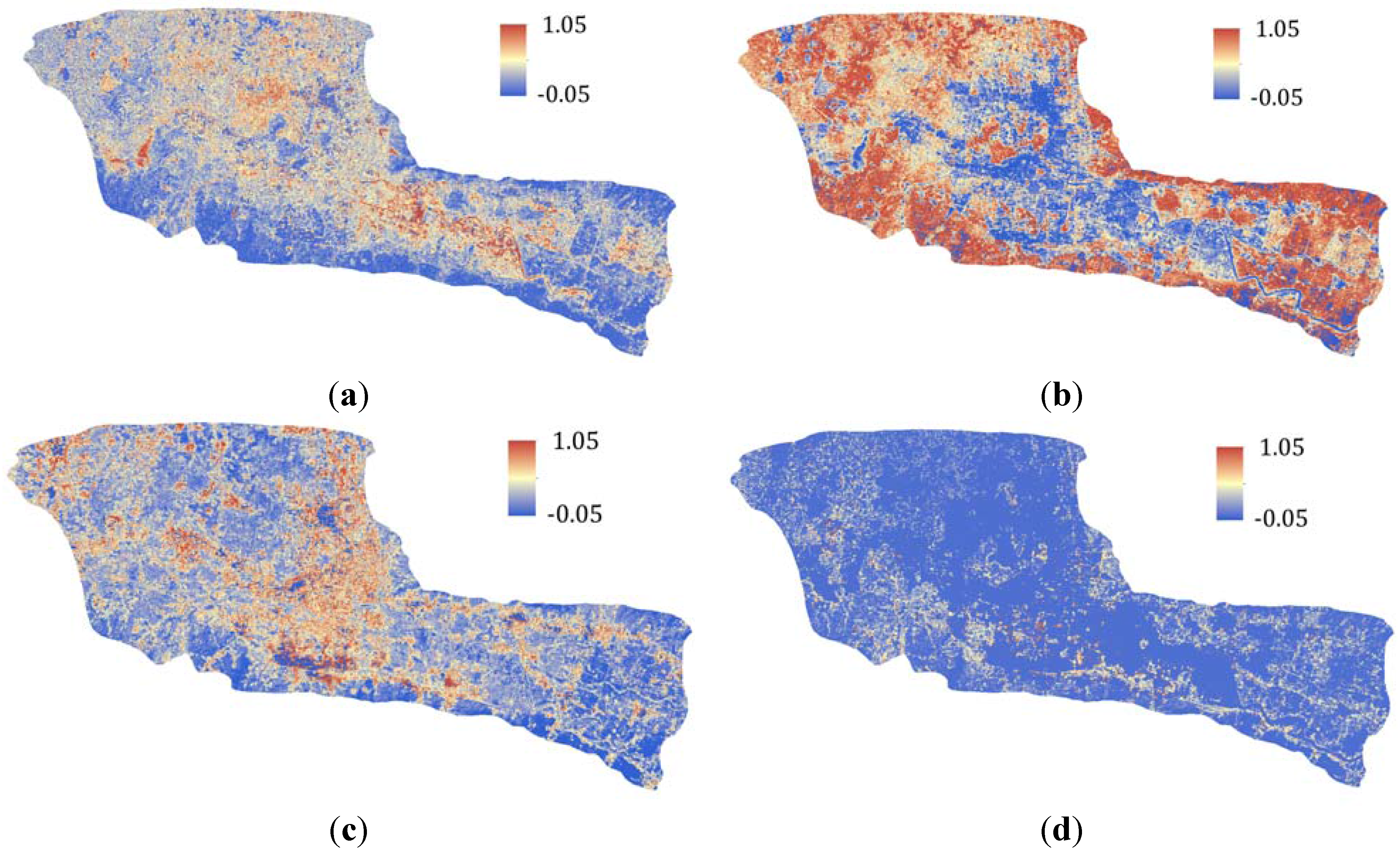
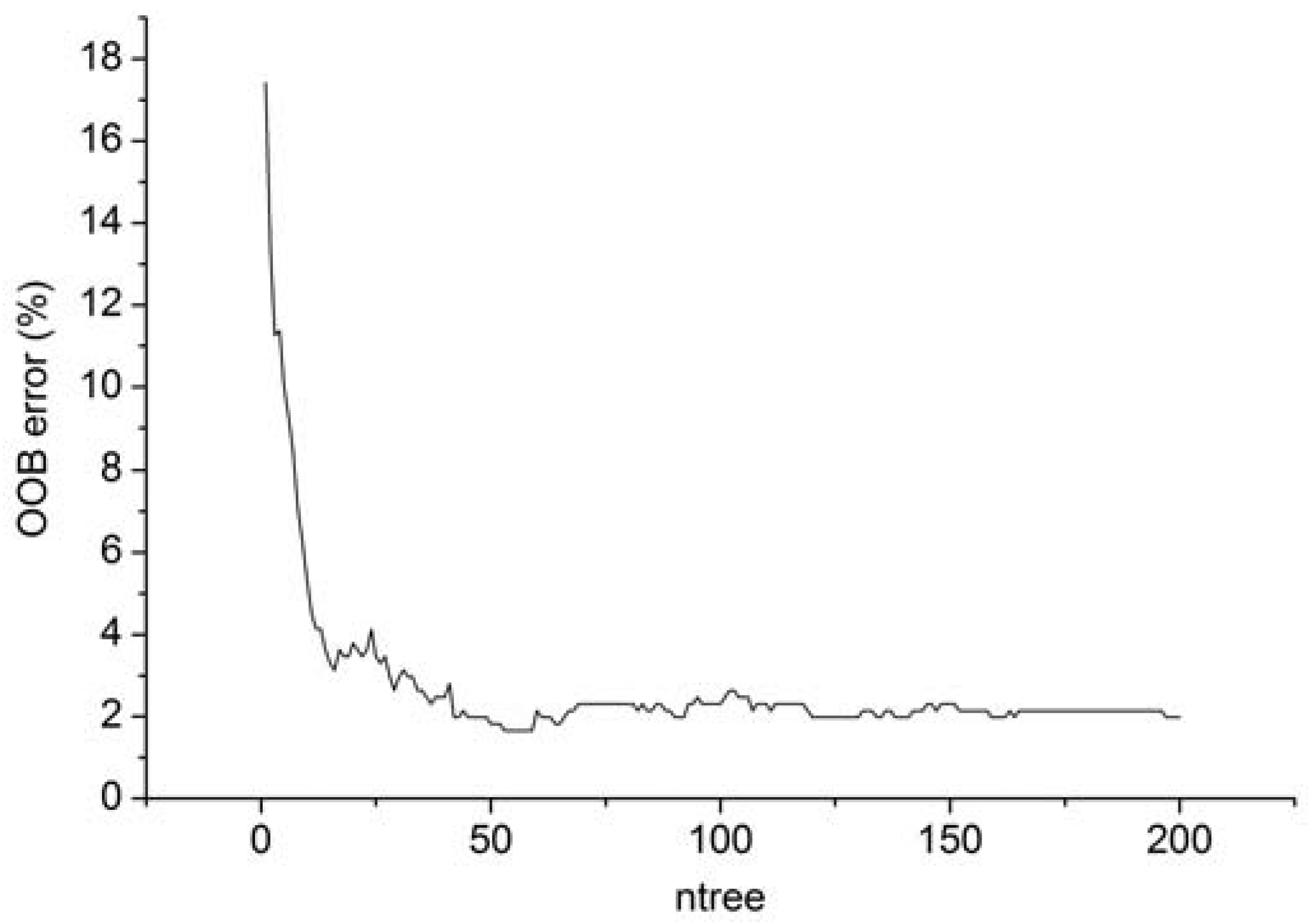
This paper proposed a hybrid method for flood mapping using medium resolution optical remote sensing data based on multiple endmember spectral mixture analysis and Random Forest classifier. A spectral library was first established using four image endmembers, including water, vegetation, impervious surface, and soil. A total of 35 optimal endmembers were selected and 3111 SMA models were constructed for each pixel to derive the fractional information. In order to increase the separability between different land cover types, the original reflectance bands, NDWI, DEM, slope, and aspect together with the fraction maps derived through MESMA were combined to construct the multi-dimensional feature space. A Random Forest classifier consisting of 200 decision trees was utilized to extract the inundated areas of Yuyao City, China. Experimental results indicated that the proposed hybrid method showed good performance with an overall accuracy of 94% and a Kappa index of 0.88. The inclusion of fractions from MESMA can improve the classification accuracy with an increase of 2.5%. Comparison experiments with other methods including maximum likelihood classifier and NDWI thresholding verified the effectiveness of the proposed method.

Above all, the hybrid method of this paper can extract inundated areas accurately using medium resolution multispectral optical data. Meanwhile, the proposed method can be expanded to the field of hyperspectral image analysis. Future studies should include more study cases to further verify the role of MESMA in the improvement of classification accuracy. A statistical sampling method should also be considered to further increase the reliability of the results of the accuracy assessment. Additionally, multi-sensor and high resolution remote sensing data are required to increase flood mapping accuracy.

References

1. Kuenzer, C.; Guo, H.; Huth, J.; Leinenkugel, P.; Li, X.; Dech, S. Flood mapping and flood dynamics of the Mekong Delta: ENVISAT-ASAR-WSM based time series analyses. Remote Sens. 2013, 5, 687–715. [Google Scholar] [CrossRef] [Green Version]
2. Kuenzer, C.; Guo, H.; Schlegel, I.; Tuan, V.Q.; Li, X.; Dech, S. Varying scale and capability of Envisat ASAR-WSM, TerraSAR-X Scansar and TerraSAR-X Stripmap data to assess urban flood situations: A case study of the Mekong Delta in Can Tho Province. Remote Sens. 2013, 5, 5122–5142. [Google Scholar] [CrossRef]
3. Schnebele, E.; Cervone, G.; Kumar, S.; Waters, N. Real time estimation of the Calgary floods using limited remote sensing data. Water 2014, 6, 381–398. [Google Scholar] [CrossRef]
4. Wang, Y.; Colby, J.D.; Mulcahy, K.A. An efficient method for mapping flood extent in a coastal floodplain using Landsat TM and DEM data. Int. J. Remote Sens. 2002, 23, 3681–3696. [Google Scholar] [CrossRef]
5. Ticehurst, C.; Guerschman, J.P.; Chen, Y. The strengths and limitations in using the daily MODIS open water likelihood algorithm for identifying flood events. Remote Sens. 2014, 6, 11791–11809. [Google Scholar] [CrossRef]
6. Martinis, S.; Twele, A. A hierarchical spatio-temporal Markov model for improved flood mapping using multi-temporal X-band SAR data. Remote Sens. 2010, 2, 2240–2258. [Google Scholar] [CrossRef]
7. Gstaiger, V.; Huth, J.; Gebhardt, S.; Wehrmann, T.; Kuenzer, C. Multi-sensoral and automated derivation of inundated areas using TerraSAR-X and ENVISAT ASAR data. Int. J. Remote Sens. 2012, 33, 7291–7304. [Google Scholar] [CrossRef]
8. Mallinis, G.; Gitas, I.Z.; Giannakopoulos, V.; Maris, F.; Tsakiri-Strati, M. An object-based approach for flood area delineation in a transboundary area using ENVISAT ASAR and LANDSAT TM data. Int. J. Digit. Earth 2013, 6, 124–136. [Google Scholar] [CrossRef]
9. Brivio, P.; Colombo, R.; Maggi, M.; Tomasoni, R. Integration of remote sensing data and GIS for accurate mapping of flooded areas. Int. J. Remote Sens. 2002, 23, 429–441. [Google Scholar] [CrossRef]
10. Wang, Y. Using Landsat 7 TM data acquired days after a flood event to delineate the maximum flood extent on a coastal floodplain. Int. J. Remote Sens. 2004, 25, 959–974. [Google Scholar] [CrossRef]
11. Amini, J. A method for generating floodplain maps using IKONOS images and DEMs. Int. J. Remote Sens. 2010, 31, 2441–2456. [Google Scholar] [CrossRef]
12. Gianinetto, M.; Villa, P. Mapping Hurricane Katrina’s widespread destruction in New Orleans using multisensor data and the normalized difference change detection (NDCD) technique. Int. J. Remote Sens. 2011, 32, 1961–1982. [Google Scholar] [CrossRef]
13. Adams, J.B.; Sabol, D.E.; Kapos, V.; Filho, R.A.; Roberts, D.A.; Smith, M.O.; Gillespie, A.R. Classification of multispectral images based on fractions of endmembers: Application to land cover change in the Brazilian Amazon. Remote Sens. Environ. 1995, 52, 137–154. [Google Scholar] [CrossRef]
14. Foody, G.M. Estimation of sub-pixel land cover composition in the presence of untrained classes. Comput. Geosci. 2000, 26, 469–478. [Google Scholar] [CrossRef]
15. Foody, G.M.; Campbell, N.A.; Trodd, N.M.; Wood, T.F. Derivation and applications of probabilistic measures of class membership from the maximum-likelihood classification. Photogramm. Eng. Remote Sens. 1992, 58, 1335–1341. [Google Scholar]
16. Lu, D.; Weng, Q. Spectral mixture analysis of the urban landscape in Indianapolis with Landsat ETM+ imagery. Photogramm. Eng. Remote Sens. 2004, 70, 1053–1062. [Google Scholar] [CrossRef]
17. Lu, D.; Batistella, M.; Moran, E.; Mausel, P. Application of spectral mixture analysis to Amazonian land-use and land-cover classification. Int. J. Remote Sens. 2004, 25, 5345–5358. [Google Scholar] [CrossRef]
18. Tooke, T.R.; Coops, N.C.; Goodwin, N.R.; Voogt, J.A. Extracting urban vegetation characteristics using spectral mixture analysis and decision tree classifications. Remote Sens. Environ. 2009, 113, 398–407. [Google Scholar] [CrossRef]
19. Zhang, Y.; Lu, D.; Yang, B.; Sun, C.; Sun, M. Coastal wetland vegetation classification with a Landsat Thematic Mapper image. Int. J. Remote Sens. 2011, 32, 545–561. [Google Scholar] [CrossRef]
20. Roberts, D.A.; Gardner, M.; Church, R.; Ustin, S.; Scheer, G.; Green, R.O. Mapping chaparral in the Santa Monica Mountains using multiple endmember spectral mixture models. Remote Sens. Environ. 1998, 65, 267–279. [Google Scholar] [CrossRef]
21. Liu, T.; Yang, X. Mapping vegetation in an urban area with stratified classification and multiple endmember spectral mixture analysis. Remote Sens. Environ. 2013, 133, 251–264. [Google Scholar] [CrossRef]
22. Quintano, C.; Fernández-Manso, A.; Roberts, D.A. Multiple Endmember Spectral Mixture Analysis (MESMA) to map burn severity levels from Landsat images in Mediterranean countries. Remote Sens. Environ. 2013, 136, 76–88. [Google Scholar] [CrossRef]
23. Gan, M.; Deng, J.; Zheng, X.; Hong, Y.; Wang, K. Monitoring urban greenness dynamics using multiple endmember spectral mixture analysis. PLoS ONE 2014, 9, e112202. [Google Scholar] [CrossRef] [PubMed]
24. Michishita, R.; Jiang, Z.; Xu, B. Monitoring two decades of urbanization in the Poyang Lake area, China through spectral unmixing. Remote Sens. Environ. 2012, 117, 3–18. [Google Scholar] [CrossRef]
25. Powell, R.L.; Roberts, D.A.; Dennison, P.E.; Hess, L.L. Sub-pixel mapping of urban land cover using multiple endmember spectral mixture analysis: Manaus, Brazil. Remote Sens. Environ. 2007, 106, 253–267. [Google Scholar] [CrossRef]
26. Franke, J.; Roberts, D.A.; Halligan, K.; Menz, G. Hierarchical multiple endmember spectral mixture analysis (MESMA) of hyperspectral imagery for urban environments. Remote Sens. Environ. 2009, 113, 1712–1723. [Google Scholar] [CrossRef]
27. Myint, S.W.; Okin, G.S. Modelling land-cover types using multiple endmember spectral mixture analysis in a desert city. Int. J. Remote Sens. 2009, 30, 2237–2257. [Google Scholar] [CrossRef]
28. Breiman, L. Random forests. Mach. Learn. 2001, 45, 5–32. [Google Scholar] [CrossRef]
29. Feng, Q.; Liu, J.; Gong, J. UAV remote sensing for urban vegetation mapping using random forest and texture analysis. Remote Sens. 2015, 7, 1074–1094. [Google Scholar] [CrossRef]
30. Feng, Q.; Liu, J.; Gong, J. Urban flood mapping based on unmanned aerial vehicle remote sensing and random forest classifier—A case of Yuyao, China. Water 2015, 7, 1437–1455. [Google Scholar] [CrossRef]
31. Immitzer, M.; Atzberger, C.; Koukal, T. Tree species classification with random forest using very high spatial resolution 8-band WorldView-2 satellite data. Remote Sens. 2012, 4, 2661–2693. [Google Scholar] [CrossRef]
32. Rodriguez-Galiano, V.F.; Chica-Olmo, M.; Abarca-Hernandez, F.; Atkinson, P.M.; Jeganathan, C. Random forest classification of mediterranean land cover using multi-seasonal imagery and multi-seasonal texture. Remote Sens. Environ. 2012, 121, 93–107. [Google Scholar] [CrossRef]
33. Ghosh, A.; Sharma, R.; Joshi, P.K. Random forest classification of urban landscape using Landsat archive and ancillary data: Combining seasonal maps with decision level fusion. Appl. Geol. 2014, 48, 31–41. [Google Scholar] [CrossRef]
34. Rosa, D.L.; Wiesmann, D. Land cover and impervious surface extraction using parametric and non-parametric algorithms from the open-source software R: An application to sustainable urban planning in Sicily. GISci. Remote Sens. 2013, 50, 231–250. [Google Scholar]
35. Hayes, M.H.; Miller, S.N.; Murphy, M.A. High-resolution landcover classification using Random Forest. Remote Sens. Lett. 2014, 5, 112–121. [Google Scholar] [CrossRef]
36. Mishra, N.B.; Crews, K.A. Mapping vegetation morphology types in a dry savanna ecosystem: Integrating hierarchical object-based image analysis with random forest. Int. J. Remote Sens. 2014, 35, 1175–1198. [Google Scholar] [CrossRef]
37. Puissant, A.; Rougier, S.; Stumpf, A. Object-oriented mapping of urban trees using random forest classifiers. Int. J. Appl. Earth Obs. 2014, 26, 235–245. [Google Scholar] [CrossRef]
38. Xu, L.; Li, J.; Brenning, A. A comparative study of different classification techniques for marine oil spill identification using RADARSAT-1 imagery. Remote Sens. Environ. 2014, 141, 14–23. [Google Scholar] [CrossRef]
39. Feng, Q.; Gong, J. Destriping remotely sensed data using anisotropic diffusion in wavelet domain. In Proceedings of 2014 4th IEEE International Conference on Information Science and Technology (ICIST), Shenzhen, China, 26–28 April 2014; pp. 316–319.
40. Vermote, E.F.; Tanre, D.; Deuze, J.L.; Herman, M.; Morcrette, J. Second simulation of the satellite signal in the solar spectrum, 6S: An overview. IEEE Trans. Geosci. Remote Sens. 1997, 35, 675–686. [Google Scholar] [CrossRef]
41. Roberts, D.A.; Halligan, K.; Dennison, P.E. VIPER Tools User Manual (Version1.5). Available online: http:// www.vipertools.org/ (assessed on 12 February 2015).
42. American Museum of Natural History, Center for Biodiversity and Conservation. Available online: http://biodiversityinformatics.amnh.org/ (assessed on 12 February 2015).
43. Random Forest Classification. Available online: http://bitbucket.org/rsbiodiv/randomforest classification/ (assessed on 12 February 2015).
44. McFeeters, S. The use of the normalized difference water index (NDWI) in the delineation of open water features. Int. J. Remote Sens. 1996, 17, 1425–1432. [Google Scholar] [CrossRef]
45. Boschetti, M.; Nutini, F.; Manfron, G.; Brivio, P.; Nelson, A. Comparative analysis of normalised difference spectral indices derived from MODIS for detecting surface water in flooded rice cropping systems. PLoS ONE 2014, 9, e88741. [Google Scholar] [CrossRef] [PubMed]
46. Chen, D.; Stow, D. The effect of training strategies on supervised classification at different spatial resolutions. Photogramm. Eng. Remote Sens. 2002, 68, 1155–1162. [Google Scholar]
47. Juan, D.; Sandra, G. Development of a sub-pixel analysis method applied to dynamic monitoring of floods. Int. J. Remote Sens. 2012, 33, 2277–2295. [Google Scholar]
48. Memon, A.; Muhammad, S.; Rahman, S.; Haq, M. Flood monitoring and damage assessment using water indices: A case study of Pakis tan flood-2012. Egypt. J. Remote Sens. Space Sci. 2015, 18, 99–106. [Google Scholar] [CrossRef]
49. Rogers, A.; Kearney, M. Reducing signature variability in unmixing coastal marsh thematic mapper scenes using spectral indices. Int. J. Remote Sens. 2004, 25, 2317–2335. [Google Scholar] [CrossRef]
50. Ji, L.; Zhang, L.; Wylie, B. Analysis of dynamic thresholds for the normalized difference water index. Photogramm. Eng. Remote Sens. 2009, 75, 1307–1317. [Google Scholar] [CrossRef]