1. Introduction
Global downward surface shortwave radiation is defined as the irradiance in the solar spectrum reaching the Earth’s surface per unit of surface [
1], also known as solar radiation (Rs and solar radiation hereafter). Knowledge of spatiotemporal distributions of this parameter is essential for understanding numerous processes in the climate system, such the water cycle or plant photosynthesis [
2]. In this regard, Rs is crucial in hydrology, playing a key role in the modelling of evapotranspiration (ET) as well as air temperature [
3,
4,
5,
6,
7,
8]. Moreover, it is a critical input parameter to crop monitoring systems that rely on agrometeorologic models [
9,
10]. Finally, R
s is essential for diverse socioeconomic sectors, such as the production of energy from solar energy systems [
2,
11,
12,
13,
14,
15].
Time series of R
s data at specific locations can be obtained from a variety of sources: measured at weather stations, modelled using other, more readily-available meteorological observations (e.g., sunshine duration, cloud cover and air temperature range), numerical weather prediction (NWP) models and reanalysis and satellite observations [
10]. However, R
s estimates from weather stations alone are not in general sufficient to integrate solar energy onto accurate gridded R
s time series at high spatial resolutions, as this parameter is most difficult to obtain due to the limited number of weather stations that measure this variable [
9,
10,
15]. In contrast, R
s can be obtained easily by means of NWP and satellite observations. Both sources of information are able to provide high spatial and temporal resolution information over large areas. NWP models and their parameters are available for weather prediction and are the basis of solar yield forecasts as they are most appropriate for solar radiation forecasting from a few hours to days ahead, and of particular importance for application in the energy market, where day-ahead power trading plays a major role in many countries [
13,
15]. Among the different NWP models, mesoscale models can be run over a smaller area when compared with global scale models, including additional details in its physics. Therefore, provided sufficient computing power, these models can be used to forecast solar irradiance over a wide area with high temporal and spatial resolution [
13]. On the other hand, operational satellite systems provide valuable information on atmospheric parameters at regular intervals on a global scale. Nowadays, there is a wide variety of satellites, both geostationary and sun-synchronous, from which R
s can be retrieved regionally or globally such as Terra/Aqua Moderate Resolution Imaging Spectroradiometer (MODIS), the National Oceanic and Atmospheric Administration’s (NOAA) Advanced Very High Resolution Radiometer (AVHRR), the Geostationary Operational Environmental Satellites (GOES) or the Meteosat Second Generation (MSG) Spinning Enhanced Visible and Infrared Imager sensor (SEVIRI). Unlike sun-synchronous sensors, geostationary sensors are especially interesting because of their high temporal resolution, which facilitates mapping of R
s at intervals of 15–30 min over large areas [
3]. Among all this satellite data, R
s estimates derived from the MSG SEVIRI data product DSSF (Downwelling Surface Short-wave Radiation Flux), have already been evaluated for different areas over Europe (see, e.g., [
3,
10,
16,
17], and will be used in the current study, as it is described in the next paragraph. Comparing satellite methods with NWP models, the latter have some potential advantages over the former, such as the possibility to evaluate solar radiation at global scale over longer periods than satellites. Additionally, NWP models perform a comprehensive simulation of the whole atmospheric system, including ancillary variables such as wind, temperature or relative humidity [
18]. However, previous studies have shown that the accuracy achieved using NWP models when computing the surface solar radiation is still significantly less than that obtained using satellite-based models [
10,
19,
20,
21]. In these studies, reanalysis data has usually been used to be contrasted with satellite data, due to the fact that in reanalysis one NWP model with fixed parameters is employed for the entire time series, which improves the temporal consistency of retrieved climate variables [
10]. In contrast, NWP models and their parameters are frequently updated for weather prediction, thus providing crucial meteorological data, including solar radiation, in a real-time environment. From this point of view, the validation of operational NWP solar radiation forecasts is of significant importance for solar resource assessment and management. Even though a few studies have been performed in this regard, the Weather Research and Forecasting (WRF; [
22]) mesoscale model has been used for solar yield forecasting in Spain [
13,
15,
18]. In this regard, [
23,
24] have evaluated the WRF and RAMS forecasted R
s in Southern Italy. In addition, a comprehensive study conducted by [
15] dealt with the comparison of several NWP solar irradiance forecasts in the US, Canada and Europe. Finally, [
25,
26] have evaluated in these same terms the NWP meteorological mesoscale model (MSM) developed by the Japan Meteorological Agency (JMA) over Japan.
In the current work, we present a regional-scale evaluation of different R
s datasets: NWP forecasts, based on the Regional Atmospheric Modeling System (RAMS; [
27,
28]), and a satellite-derived product, the DSSF algorithm, for the Valencia Region (eastern Spain). In this regard, RAMS was implemented within an operational forecast environment within this area of study for the winter 2010–2011 and the summer 2011, using the most recent versions of this model, RAMS 4.4 (RAMS44 hereafter) and RAMS 6.0 (RAMS60 hereafter) [
29,
30,
31,
32,
33]. For these two seasons, this operational system was providing R
s forecasts for different locations distributed along the area of study (
Figure 1), with a temporal horizon of three consecutive days (today, tomorrow and the day after tomorrow) and two daily initializations of the model.
Figure 1.
Simulation domain configuration and distribution of the meteorological weather stations used in the validation of solar radiation estimates depending on the terrain class: flat (closed square) and hilly (closed circle) in addition to the orography simulated by Regional Atmospheric Modeling System (RAMS) within the finer domain (D3).
Therefore, the main aim of this paper is double. On the one hand, we present a comprehensive evaluation of both the RAMS-forecasted Rs and the DSSF product. In this sense, this mesoscale model outputs and this satellite-based data are compared with surface meteorological observations available within the area of study. On the other hand, the usage of different approaches to obtain Rs estimates will permit us to contrast these two sources of data. The Rs performance and accuracy are then evaluated for these datasets segmented based on terrain classes (flat or hilly), and taking into account the corresponding sky condition (clear or cloudy) together with considering all sky conditions. Additionally, the evaluation process is performed for the winter 2010–2011 and the summer 2011, separately. Winter is defined by the months December–February (DJF) and summer from June to August (JJA). Finally, both RAMS44 and RAMS60 and their two daily initializations are compared as well, so as to acquire a full description of the differences between the most recent versions of the model and the effect of the spin-up on the simulation results.
The paper is structured as follows:
Section 2 presents the characterization of the study area, as well as the different datasets used in this study. The evaluation methodology is given in
Section 3, while
Section 4 is devoted to the analysis of the results. In addition, the discussion of these results is presented in
Section 5, particularly including a comparison of those achieved in the current work with those obtained in previous studies. Finally, some concluding remarks are provided in
Section 6.
3. Evaluation Methodology
Both the DSSF product and the RAMS forecasts are evaluated with respect to ground observations at hourly and daily time scales. Considering the DSSF product, a standard day consists of 48 files in HDF5 format, one image every 30 min. This has required aggregation of the DSSF product, available at 30 min intervals. In order to compare the satellite-derived and RAMS-forecasted R
s with the surface weather stations, both DSSF and model outputs were extracted at the corresponding locations. In the case of the RAMS model, we developed a software tool to extract and store, for each daily simulation within the period of study (winter of 2010–2011 and summer of 2011), the hourly simulated R
s, at each selected weather station location using Domain 3 of the simulation (
Figure 1). This surface data was then stored in a database for the three days of simulation, the two daily RAMS initializations and the two RAMS versions [
33]. In the case of the DSSF model, the daily 48 files were downloaded and processed for the winter 2010–2011 and the summer 2011, even though there are days that have fewer files within the daily cycle. To minimize the impact of data re-sampling due to reprojection, the analysis was carried out in the original projection and spatial resolution of the DSSF product [
3]. Once the DSSF product was imported, data extraction was performed using the “nearest point” interpolation in space to the meteorological station locations.
The evaluation procedure used in the current study follows basically that used in [
3]. DSSF algorithm performance is analysed under both clear and cloudy sky conditions for hourly and daily evaluation. In the hourly-basis assessment, each hour and pixel record is flagged in terms of cloudy mask and DSSF algorithm with the aim of reporting the corresponding sky conditions. A pixel masked as clear corresponds to a pixel with both the two 30 min intervals DSSF files classified as clear (
i.e., a pixel masked as clear both at 12:00 UTC and 12:30 UTC). On the other hand, a pixel masked as cloudy corresponds to a pixel with both the two 30 min intervals DSSF files classified as cloudy. Besides, pixels with different quality flags for a specific hour were excluded in the analysis (
i.e., a pixel masked as clear at 12:00 UTC and cloudy at 12:30 UTC). In the daily-basis assessment, the hourly generated files are used to compute the daily R
s average. In this case, the sky condition is also considered. Thus, each day and pixel record is flagged in this sense. To do this, we have used the criterion proposed by [
3], which considers a clear-sky day at a given pixel if ≥80% of the time samples between dawn and dusk were cloud free. Moreover, they propose that at least 90% of the potential images within a day must be available as criteria for computation of daily average R
s from the DSSF product. These hourly and daily cloudy and clear sky conditions obtained for DSSF are then exported to the RAMS results and the surface-based data. Therefore, the observed and forecasted hourly records have been recalculated to daytime averages as well.
The assessment of the DSSF product and the RAMS forecasts is performed using several statistical indexes and measures of error, such as the mean bias error (MBE), the mean absolute error (MAE), the root mean square error (RMSE) and the index of agreement (IoA), as defined by the following equations:
where
N represents the number of observations included in the calculation.
F represents the simulated value and
O the observation, while
O correspond to the time average observed.
The Mean Bias Error (MBE) is defined as the average of the simulated value minus the observed value and quantifies the systematic error of the model or estimator, the RMSE is used as a measure of the accuracy, and corresponds to the square root of the individual differences between values simulated by a model or an estimator and the observed values, the Mean Absolute Error (MAE) indicates the magnitude of the average error. Finally, the Index of Agreement (IoA), is a modified correlation coefficient that measures the degree to which a model's prediction is free of error. A value of 0 means complete disagreement while a value of 1 implies a perfect agreement.
In addition, the relative errors of the MBE, MAE and RMSE (rMBE, rMAE and rRMSE, respectively) are also calculated as the ratio between the corresponding statistical score and the mean ground observations.
The different accuracy statistics for solar radiation are then computed at hourly and daily time steps. The hourly evaluation considers all hourly records within the corresponding season: winter 2010–2011 (DJF) and summer 2011 (JJA). Thus, the observed and forecasted solar radiation for each hour within each day in the period of these seasons are compared. As mentioned previously, the available information has been divided by areas (flat and hilly terrain), and by sky condition (clear, cloudy and all skies). On the other hand, the daily evaluation includes the same statistical scores but taking into account the daily average records within these seasons of the year, that is, the average observed and forecasted solar radiation for each day within the corresponding season. In the case of RAMS, both evaluation time steps are performed independently for all days of simulation: today, tomorrow and the day after tomorrow (D1–D3 respectively), the two versions of the model (4.4 and 6.0) and the two daily initialization (00Z and 12Z). Considering this distribution of the available data, the next format is used throughout the text: (Day:RAMS Version-RAMS Initialization). For instance, D1:4.4-00Z represents the results computed (within the daily or hourly evaluation) for the first day of simulation using the 00Z daily initialization of RAMS44.
Finally, the different accuracy measurements and errors presented in the current section are shown with one significant figure only if the first two significant figures of the error are higher than 25 and with two significant figures otherwise.
5. Discussions and Outlook
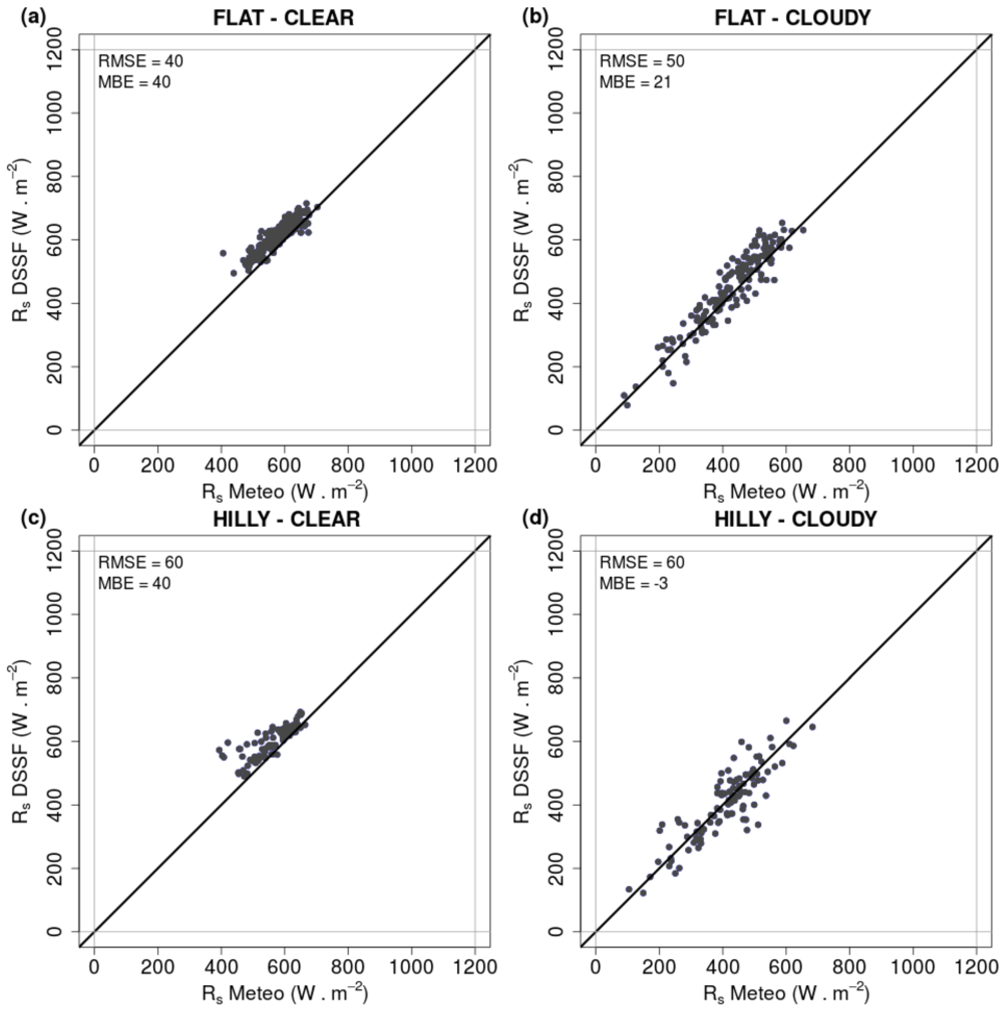
Results presented in the current study at the daily time step for the DSSF product are consistent with those found in the literature. In this regard, and considering a daily evaluation, [
3] found an averaged RMSE and MAE for the 2008–2010 period of 30 W·m
−2 and 20 W·m
−2, respectively at flat sites and under clear sky conditions. Cloudy conditions over these locations yielded an averaged RMSE and MAE considering the whole 2008–2010 period of 40 W·m
−2 and 30 W·m
−2, respectively. On the other hand, clear sky conditions yielded an averaged RMSE and MAE of 40 W·m
−2 and 30 W·m
−2, respectively, for hilly sites, while these values rises up to 50 W·m
−2 and 40 W·m
−2, respectively, under cloudy conditions. [
17] found an RMSE of 40 W·m
−2 and 110 W·m
−2 under clear and cloudy skies, respectively, using data from six European ground measurement stations from 2004 to 2006. In addition, [
50] used 13 weather stations from 2008 to 2009 in Belgium, yielding an RMSE of 40 W·m
−2 and 90 W·m
−2 considering stations over flat terrain, clear and cloudy conditions, respectively. Separating the winter from the summer season, similar results are found in the current study. For example, in the case of the winter time, the current study yields an average RMSE and MAE of 25 W·m
−2 and 20 W·m
−2, respectively, at flat sites and under clear sky conditions, 40 W·m
−2 and 30 W·m
−2, respectively, at flat sites and under cloudy sky conditions, 40 W·m
−2 and 30 W·m
−2, respectively, at hilly sites and under clear sky conditions, 40 W·m
−2 and 30 W·m
−2, respectively, at hilly sites and under cloudy sky conditions (
Table 3). Results during the summer produce slightly larger errors than those found within the winter season.
Considering an hourly evaluation for the whole 2008–2010 period, [
3] found an average RMSE and MAE of 40 W·m
−2 and 30 W·m
−2, respectively, over flat terrain under clear sky conditions, while cloudy conditions over these locations yielded an averaged RMSE and MAE considering of 90 W·m
−2 and 60 W·m
−2, respectively. On the contrary, clear sky conditions yielded an averaged RMSE and MAE of 60 W·m
−2 and 40 W·m
−2, respectively, for hilly sites, while these values rises up to 110 W·m
−2 and 70 W·m
−2, respectively, under cloudy conditions. Separating the winter from the summer season, similar results are found in the current study. For example, taking into account the winter season, the current study yields an average RMSE and MAE of 40 W·m
−2 and 30 W·m
−2, respectively, at flat sites and under clear sky conditions, 70 W·m
−2 and 50 W·m
−2, respectively, at flat sites and under cloudy sky conditions, 50 W·m
−2 and 40 W·m
−2, respectively, at hilly sites and under clear sky conditions, 80 W·m
−2 and 60 W·m
−2, respectively, at hilly sites and under cloudy sky conditions (
Table 6). Once again, results during the summer produce larger errors than those found within the winter season.
Although previous studies dealt in general with the whole dataset [
17] or considering the whole year [
3], a monthly evaluation was performed as well. Considering a monthly aggregation of the DSSF data, [
17] found no clear seasonal bias dependence in the results considering cloudy sky data. In contrast, for the clear sky case a seasonal trend of the monthly biases was obtained, even though the MBE is in general very small and exhibits slightly positive values of less than 10 W·m
−2. In this regard, for the clear sky estimates a seasonal trend of the monthly values was perceived (slight underestimation in winter and overestimation in summer). Although no monthly aggregation has been performed in the current study for the DSSF data, the evaluation carried out permits to highlight the seasonal trend obtained within the Valencia Region. In this sense, a similar tendency as the one found in those previous studies is perceived as well. Thus, the MBE is positive during the summer, meaning an overestimation of the observed R
s, while this score is negative during the winter season, indicating an underestimation of the observed R
s.
On the other hand, the slightly lowest absolute errors obtained by [
3], when compared to those obtained in the current work, could be related to a compensation of errors in considering the whole year. In this sense, as it was pointed out by [
17], when considering the statistics for individual months, more important biases with a positive or negative sign occur which tend to cancel out over the whole period. According this work, a possible explanation for the behaviour of the clear sky bias could potentially be related to an insufficient parameterization of the effects of aerosols, which are currently parameterized with a fixed visibility value of 20 km and therefore their variations are not taken into account.
Previous studies have shown that R
s from reanalysis data produces significantly less accuracy than satellite-based models [
10,
19,
20,
21]. However, few studies have been focused on the comparison of operational NWP models with satellite-derived data [
13,
15,
23,
24,
25,
26]. These previous works have shown that, as in the case of reanalysis data, forecast models overestimate R
s in general compared to the ground-based measurements. For example, using the WRF model in Andalusia (southern Spain) in a seasonal evaluation [
13], a positive MBE is obtained for all seasons of the year, with values around 40 W·m
−2 under clear sky conditions and higher than 100 W·m
−2 in the presence of cloudiness. Additionally, the RMSE shows values of about 100 W·m
−2 under clear sky conditions and higher than 150 W·m
−2 considering cloudy cloudiness, reaching values up to 300 W·m
−2. Comparing the relative errors, [
13] found a large difference between cloudy and overcast conditions. Although this work divided cloudiness in two categories, cloudy and overcast, we only consider here a category to define this parameter, based on the DSSF product. The results obtained in the current study under cloudy conditions show values in between those found by [
13], based on cloudy and overcast conditions. Thus, considering the total cloudiness could also be the reason for the higher dispersion observed in
Figure 4 and
Figure 5 when using the RAMS model under cloudy conditions. Besides, RMSE rises over hilly terrain within both the summer and the winter seasons. In general, a higher accuracy in terms of the RMSE statistical score is obtained in the summer over flat terrain compared to that obtained for the winter season. In contrast, similar results are found in this accuracy estimation over hilly terrain contrasting these two seasons of the year. These RMSE results are rather similar to those obtained in the current study in terms of magnitude. However, comparing the RMSE for the winter and the summer seasons, WRF produces similar results in both seasons, with even lower values during the summer when considering all sky conditions, in contrast to the RMSE results produced by RAMS in the current work. In addition, although the MBE trend obtained in the current study is the same as the one obtained by [
13], thus producing an overestimation of the observations, a significant divergence appears in term of the MBE score during the winter season. In this sense, RAMS produces an underestimation of the observations, in accordance with the MBE obtained using the DSSF product. In contrast, [
13] found a positive MBE using WRF for the four seasons of the year. Additionally, [
25,
26] have also obtained a different trend in the MBE statistical score when comparing the summer with the winter seasons, using the Japan Meteorological Agency mesoscale model (MSM). However, although the current study shows an underestimation of the observations using the RAMS model during the winter season, the MSM produces an overestimation of the observations during this season of the year over Japan. In contrast, the opposite trend has been found within the summer season. In any case, and as it has also been found in the current study, MSM presents larger RMSE errors during the summer season, with values around 100 W·m
−2, when compared to those obtained during the winter, higher than 150 W·m
−2. This outcome contrasts with the RMSE values found by [
13] comparing the winter and the summer seasons using the WRF model over southern Spain and considering all sky conditions, as it has been pointed out previously.
Finally, [
23] have also found an overestimation of about 30 W·m
−2 for both RAMS and WRF forecasted R
s with respect to the ground based sensor during the summer 2013 in Southern Italy, with a global RMSE of 100 W·m
−2. In the same terms, [
24] have evaluated the RAMS and WRF forecasted R
s as well as the DSSF product during the period June 2013–December 2013 in Southern Italy. Once again, they have also found not only this positive bias using both NWP forecasted R
s with respect to the ground-based sensor, but also with respect to the DSSF product. Additionally, they have found an RMSE monthly-averaged of 80 W·m
−2 for the DSSF product and of 100 W·m
−2 for these weather forecast models.
The overestimation obtained by RAMS in the current study, specially during the summer season, may be related to the solar short-wave parameterization used in the current work [
45], indicating the limited ability of the RAMS model to forecast cloudy conditions in contrast to the prediction of clear skies during the summer. In this regard, RAMS appears to forecast more clear sky conditions than actually occurred. However, the opposite has also been found during the winter season (
Figure 5), and in this case, even under clear sky conditions, some cloudiness is still forecasted by this model. It is worth noting that the [
45] scheme does account for condensate in the atmosphere, but not whether it is cloud water, rain, or ice, which is a major limitation [
51]. Besides the solar short-wave parameterization, the initial soil moisture content has been revealed as an important parameter to faithfully reproduce the observed patterns using the RAMS model [
52], specifically considering the solar radiation. In this regard, moistening the soil produces a better capture of the observed cloudiness under mesoscale circulations. These sort of atmospheric conditions are the most predominant meteorological situations over the area of study during the summer [
35,
36]. Thus, the false alarms produced by RAMS and related to cloudiness (
Figure 4) within this period of the year could be related to the underestimation of this parameter based on an underestimation of the atmospheric humidity [
52], that forecasts more clear skies than those really observed. Thus, the initial soil moisture content should also be kept in mind as a likely option to include a better representation of the summer cloudiness in order to improve the RAMS-forecasted R
s under cloudy sky conditions. In contrast, the most dominant situation during the winter is that associated with northerly western circulations [
35]. In this case, it seems that RAMS advects more synoptic humidity towards the region of study, thus producing more cloudy skies than those actually observed, specially over flat terrain (
Figure 5a).
6. Conclusions
The current study presents the validation and the inter-comparison of the global solar radiation estimates provided by the satellite-based model DSSF product, and the RAMS mesoscale model over the Valencia Region, located in the Western Mediterranean coast. To perform the corresponding evaluation we have taken advantage of the RAMS results generated by the operational weather forecasting system implemented within this area of study during the winter 2010–2011 and the summer 2011. In this regard, hourly and daily solar radiation estimates have been compared to ground-based data for both seasons of the year separately and considering the seasonal data segmented based on two terrain classes (flat and hilly) and two atmospheric conditions (clear and cloudy skies). Additionally, the two most recent versions of the RAMS model have been implemented within this operational system, thus being used in the current evaluation of the solar radiation forecasts.
Evaluation has shown differences between summer and winter. In this regard, even though both DSSF and RAMS overestimate the observations during the summer, the opposite is obtained during the winter season. Considering the RAMS output, it has been shown that the forecasts accuracy tends to decrease as the simulation progresses for the two daily RAMS initializations, and the best performance has been obtained for the 12 UTC run.
Taking into account the corresponding atmospheric conditions, DSSF and RAMS produce a better accuracy under clear conditions than when considering cloudy skies for both the summer and winter seasons, specially considering the RAMS forecasts. Additionally, in some cases, particularly under cloudy skies, the RAMS forecasts provided for the second and the third day of simulation show similar errors those obtained for the first day of simulation, even better in some cases. This results has also been found in other regions of Spain using the WRF model [
13].
The results found in the current work indicate that RAMS is a valuable tool to participate in those socio-economic sectors in which the estimation of solar radiation is a key factor. However, cloud forecasts are still a challenging issue for the RAMS model. In this regard, improvements should be obtained before reliable R
s forecasts are obtained under cloudy atmospheric conditions. As it was previously pointed out, the RAMS divergences with the observations found in the current study may be related to the solar short-wave parameterization used in the current work [
45]. Additionally, the initial soil moisture content has been revealed as an important parameter to faithfully reproduce the observed patterns using the RAMS model [
52].
Finally, it should be highlighted that even though the results obtained in the current study have been obtained for a particular region, they can be regarded as representatives for regions with a similar climate, as none statistical post-processing has been performed upon the forecasts provided by the model.


