Focusing Translational Variant Bistatic Forward-Looking SAR Using Keystone Transform and Extended Nonlinear Chirp Scaling

Abstract

Bistatic Synthetic Aperture Radar (SAR) has attracted increasing attention in recent years due to its unique advantages, such as the ability of forward-looking imaging. In translational variant bistatic forward-looking SAR (TV-BFSAR), it is difficult to get a well focused image due to large range cell migration (RCM) and 2-D variation of both Doppler characteristics and RCM. In this paper, an extended azimuth nonlinear chirp scaling (NLCS) algorithm is proposed to deal with these problems. Firstly, Keystone Transform (KT) is introduced to remove the spatial-variant linear RCM, which is of great significance in TV-BFSAR. Secondly, a correction factor is multiplied to the signal in range frequency domain to compensate for the residual RCM. At last, a fourth-order filtering together with azimuth NLCS is performed in every range gate to equalize both the azimuth-variant Doppler centroid and frequency modulation rate based on the azimuth numerical fitting. The proposed method is verified by simulation and real data processing. Multiple targets are generated and focused by the method, of which the peak sidelobe ratio (PSLR) is around −13 dB and integrated sidelobe ratio (ISLR) is around −10 dB. The method is accurate and can achieve high-resolution focusing for TV-BFSAR data.

1. Introduction

In recent years, synthetic aperture radar (SAR) has become increasingly attractive in both civilian and military fields, because it can provide high-resolution day- and night-time images of the observed area, independent of weather conditions [1,2,3,4]. Typical fields of SAR applications include disaster monitoring, resources exploration, geological mapping, military reconnaissance, and so on. However, the traditional monostatic SAR cannot achieve forward-looking imaging because of its inherent characteristic [5]. The range and azimuth directions coincide with each other, and a two-dimensional image can not be obtained. This restricts the applications of SAR technology in areas such as navigation, terminal guidance, self-landing, etc. With the choice of proper geometry, bistatic SAR can image the forward-looking terrain, which is called bistatic forward-looking SAR (BFSAR). A bistatic SAR system can break through the limitations of traditional monostatic SAR in forward-looking imaging and achieve high-resolution imaging of the forward-looking terrain of the receiver. This might result in some new applications of bistatic SAR in aviation by imaging obstacles (e.g., mountains) in the flight direction which are covered by fog, rain, and clouds. With such systems, we can also improve the safety of landing airplanes by imaging the runway in undesirable weather conditions [6]. Current research and publications on BFSAR include imaging theories [7,8,9], imaging algorithms [10,11,12,13,14,15,16], and experiments [17,18,19,20,21]. In Wu J. et al. [7], BFSAR is categorized into three types: translational invariant (TI), translational variant (TV), and stationary transmitter cases. In TV mode, the transmitter and receiver move with different velocities. The spaceborne/airborne BFSAR and the airborne/missleborne BFSAR often work in this mode. In comparison with the TI mode, TV-BFSAR provides higher flexibility and mobility, which makes it suitable for more complicated applications.

Some reconstruction methods for BFSAR, such as the range-Doppler algorithm (RDA) [10,11,12], Omega-k [13,14], and back-projection [15] are ongoing. The RDA neglects the spatial variation of the secondary range compression (SRC), which is very important for BFSAR. As for the Omega-k for BFSAR, the current methods all use a monostatic Omega-k algorithm after a data conversion from bistatic to monostatic. This makes it fail for cases with large bistatic angle. In addition, because of the symmetric effect of the receiver about its flight path, the range cell migration (RCM) is severely nonlinear with cross-track coordinate. Thus, the Omega-k algorithm is actually not suitable for TV-BFSAR [22]. A back-projection algorithm is a precise way to focus the raw data of TV-BFSAR. However, because of its low computational efficiency, the applications of BFSAR in real-time navigation and reconnaissance are limited, which are the major application fields of BFSAR.

In TV-BFSAR, the RCM varies with the positions of the targets, and the linear component of RCM is the most significant which should be handled. Traditional range cell migration correction (RCMC) methods [23,24,25] operated in range frequency and azimuth time domains all use correction factor multiplication to remove the linear component of RCM. However, the linear RCMC factor is constructed by using the linear RCM of the reference target, and the spatial variance of linear RCM is neglected. So, residual linear RCM still exists for targets away from the reference target. Keystone Transform (KT) is a data reformatting technique that is generally used to correct the range walk [26] or range curvature [27] of moving targets. Because it is independent of the motion parameters, it can correct the range walk or range curvature of all targets in the scene without knowing their velocities, regardless of the target position. First-order KT has already been applied to the stationary scene data processing of bistatic SAR to remove the linear RCM in [28,29,30], but these methods neglect the residual higher-order RCM, which degrades the azimuth focusing performance. Another problem is the 2-D variation of Doppler coefficients. Different from TI-BFSAR, the Doppler coefficients in the TV case depend on the range and azimuth positions of the targets. Moreover, the target undergoes a position shift after RCMC operated in range frequency and azimuth time domain, and it further aggravates the 2-D variation. Thus, the Doppler coefficients of the targets in the same range gate should first be equalized so that these targets can be compressed with the same azimuth-matched filter. Nonlinear chirp scaling (NLCS) was first adopted by Wong and Yeo in monostatic and bistatic SAR data processing [23]. Current publications on bistatic SAR NLCS algorithm can be found in References [31,32,33,34]. In Qiu et al. [34], an azimuth NLCS algorithm based on numerical fitting is proposed to process bistatic SAR data with a stationary transmitter. However, this algorithm can only deal with the spatial variance of Doppler frequency modulation rate. In some recent publications on highly squint monostatic SAR data focusing [24,25], an extended azimuth nonlinear chirp scaling algorithm (ENLCS) has been proposed. The ENLCS can simultaneously equalize the Doppler FM rate and third-order coefficient. However, in TV-BFSAR, Doppler centroid is spatial-variant for targets in the same range gate after RCMC, and it induces a variation term into the Doppler FM rate, which is ignored in the algorithm. This deteriorates the performance of azimuth focusing. Moreover, if the spatial variation of the Doppler centroid is not removed, the magnitude of the targets away from the scene center is diminished, and the azimuth resolution is coarsened because the reference function mismatch the echo data in azimuth frequency domain.

In this paper, we first analyze the characteristic of the echo signal of TV-BFSAR. Based on the analysis, an extended azimuth NLCS algorithm is proposed to process the raw data and obtain a well-focused image of the TV-BFSAR. The algorithm aims to deal with two problems of TV-BFSAR: 2D spatial-variation of linear RCM and azimuth-variant Doppler parameters. The processing procedures are as follows. First, KT is performed in the range frequency and azimuth time domain to remove the spatial-variant linear RCM. Second, a correction factor is multiplied to the echo to compensate for the residual RCM. Then, the azimuth dependence of Doppler character and the influence of spatial-variant Doppler centroid on azimuth compression are analyzed. Polynomial approximations of Doppler centroid and FM rate are obtained by using numerical curve fitting. At last, a fourth-order filtering in the azimuth frequency domain together with NLCS is carried out to equalize the Doppler centroid and FM rate based on the above analysis. The proposed algorithm resolves the problem of the variation of linear RCM and Doppler centroid, and thus has a better imaging performance for multiple targets in the scene. This method is computationally efficient compared to time-domain methods such as back projection (BP) and achieves better focusing performance than other frequency domain methods.

The rest of the paper is organized as follows. Section 2 gives the geometric and signal model of TV-BFSAR. Section 3 presents the range processing of echo signal, including KT, range compression, and higher-order RCMC. In Section 4, the azimuth dependence of Doppler coefficients is first analyzed, and the extended NLCS is then derived in detail. The numerical simulations are given in Section 5. Section 6 presents some discussionof the proposed method, including advantages, practical limitations, and future work. Section 7 concludes the paper.

2. Signal Model

The geometric graph in Figure 1 shows the configuration of a general translational variant bistatic forward-looking SAR. The transmitter works in squint mode and the receiver works in forward-looking mode. The receiver travels along the y axis with a velocity of $V_R$, and the velocity of the transmitter is $V_T$. The transmitter and the receiver both work in stripmap mode. The angle between the flight direction of the transmitter and the receiver is α. The original coordinates of the transmitter and the receiver are $(x_T,y_T,h_T)$ and $(x_R,y_R,h_R)$, respectively. The downward-looking angle of the receiver is defined as ${\theta }_R$ and the squint angle of the transmitter is defined as ${\theta }_T$, respectively. The origin of the coordinate O is the scene center, and $P(x,y)$ is an arbitrary point target in the scene.

Supposing the transmitted signal is an linear frequency modulated (LFM) pulse, the received signal after demodulation is

$$\begin{array}{c}{S}_r(t,\tau ;x,y)={\omega }_r\left(\tau -\frac{R(t;x,y)}{c}\right){\omega }_a\left(\frac{t-t_R}{T_a}\right)\hfill \\ \times exp\left[-j2\pi \frac{R(t;x,y)}{\lambda }\right]exp\left[j\pi K_r{\left(\tau -\frac{R(t;x,y)}{c}\right)}^2\right]\hfill \end{array}$$

(1)

where ${\omega }_r$ and ${\omega }_a$ are the range and azimuth envelopes, respectively. τ is the fast time and t is the slow time. λ is the wavelength and $\lambda =c/f_c$. c is the speed of light and $f_c$ is the carrier frequency. $K_r$ represents the range FM rate, $T_a$ is the synthetic aperture time, and $t_R$ is the azimuth position of the target. $R(t;x,y)$ is the bistatic range history, which is given by

$$\begin{array}{c}\hfill R(t;x,y)=R_R(t;x,y)+R_T(t;x,y)\end{array}$$

(2)

The range histories with respect to target $P(x,y)$ of the receiver and the transmitter are:

$$\begin{array}{c}\hfill R_R(t;x,y)=\sqrt{r_{0R}^2+V_R^2{(t-t_R)}^2-2r_{0R}{V}_R(t-t_R)cos{\theta }_R}\end{array}$$

(3)

$$\begin{array}{c}\hfill R_T(t;x,y)=\sqrt{r_{0T}^2+V_T^2{(t-t_T)}^2-2r_{0T}{V}_T(t-t_T)cos{\theta }_T}\end{array}$$

(4)

where $r_{0R}$ and $r_{0T}$ are the slant ranges of target P to the receiver and transmitter at $t_R$ and $t_T$, respectively. $t_R=y/V_R$ and $t_T=y/V_{T}cos\alpha$ are the beam center crossing time of the receiver and the transmitter, respectively. From Figure 1, $r_{0R}$ and $r_{0T}$ are given by

$$\begin{array}{c}\hfill r_{0R}\left(x\right)=\sqrt{x^2+y_R^2+h_R^2}\end{array}$$

(5)

$$\begin{array}{c}\hfill r_{0T}(x,y)=\sqrt{{\left[x-(x_T+ytan\alpha )\right]}^2+y_T^2+h_T^2}\end{array}$$

(6)

After range Fourier transform, the signal in the range frequency domain is given by:

$$\begin{array}{c}\hfill S_{r1}(t,f_{\tau };x,y)={\omega }_r\left(\frac{f_{\tau }}{K_r}\right){\omega }_a\left(\frac{t-t_R}{T_a}\right)\times exp\left\{-j\pi \frac{{f_{\tau }}^2}{K_r}\right\}exp\left\{-j2\pi \frac{f_{\tau }+f_c}{c}R(t;x,y)\right\}\end{array}$$

(7)

Expanding $R_R(t;x,y)$ and $R_T(t;x,y)$ (jointly denoted as $R_{R,T}(t;x,y)$ for simplicity) at $t_R$ and $t_T$ (jointly denoted as $t_{R,T}$ for simplicity) into Taylor series and keeping up to third-order terms yields

$$\begin{array}{c}\hfill R_{R,T}(t;x,y)\approx r_{0R,0T}+A_{R,T}(t-t_{R,T})+\frac{B_{R,T}}{2}{(t-t_{R,T})}^2+\frac{C_{R,T}}{6}{(t-t_{R,T})}^3\end{array}$$

(8)

where $A_{R,T}$, $B_{R,T}$, and $C_{R,T}$ are the expanding coefficients.

$$\begin{array}{c}\hfill A_{R,T}=-V_{R,T}cos{\theta }_{R,T}\end{array}$$

(9)

$$\begin{array}{c}\hfill B_{R,T}=\frac{V_{R,T}^2{sin}^2{\theta }_{R,T}}{r_{0R,0T}}\end{array}$$

(10)

$$\begin{array}{c}\hfill C_{R,T}=3\frac{V_{R,T}^3{sin}^2{\theta }_{R,T}cos{\theta }_{R,T}}{r_{0R,0T}^2}\end{array}$$

(11)

In bistatic forward-looking SAR, the absolute values of $B_{R,T}$ and $C_{R,T}$ are much smaller than that of $A_{R,T}$. Thus, the RCM components caused by B and C are much smaller than that of A, and linear range cell migration (LRCM) is more significant than higher-order RCM, which will be illustrated in Section 5.

3. LRCMC via Keystone Transform and Higher–Order RCMC

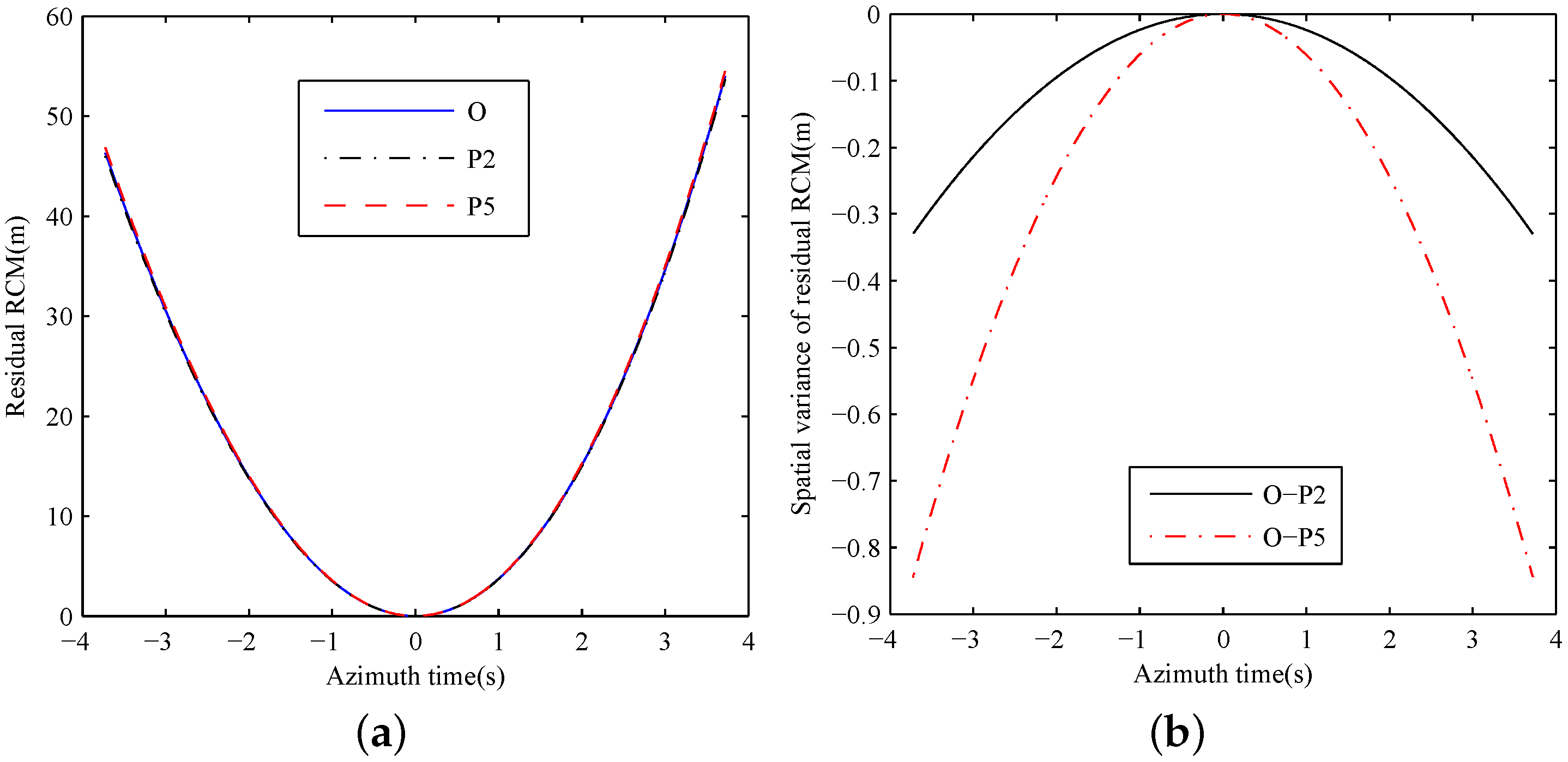
In this section, we consider the problem of RCM and range compression. As mentioned above, the main part of range cell migration is linear RCM. Thus, KT is first introduced to deal with the spatial-variant LRCM, and range compression is carried out after KT. Then, to compensate for the residual RCM, a third-order phase term of azimuth time variable is multiplied to the echo.

3.1. Linear RCMC

Substituting (Equation (8)) into Equation (2), $R(t;x,y)$ is rewritten as follows

$$\begin{array}{c}\hfill R(t;x,y)=R(0;x,y)+A^{\prime }t+\frac{B^{\prime }}{2}{t}^2+\frac{C^{\prime }}{6}{t}^3\end{array}$$

(12)

where

$$\begin{array}{c}\hfill R(0;x,y)=r_{0R}-A_R{t}_R+\frac{B_R}{2}{t}_R^2-\frac{C_R}{6}{t}_R^3+r_{0T}-A_T{t}_T+\frac{B_T}{2}{t}_T^2-\frac{C_T}{6}{t}_T^3\end{array}$$

(13)

$$\begin{array}{c}\hfill A^{\prime }=A_R-B_R{t}_R+\frac{C_R{t}_R^2}{2}+A_T-B_T{t}_T+\frac{C_T{t}_T^2}{2}\end{array}$$

(14)

$$\begin{array}{cc}\hfill B^{\prime }& =B_R-C_R{t}_R+B_T-C_T{t}_T\hfill \end{array}$$

(15)

$$\begin{array}{cc}\hfill C^{\prime }& =C_R+C_T.\hfill \end{array}$$

(16)

$R(0;x,y)$ represents the bistatic slant range at $t=0$.

After the slant range expansion in Equation (12), the phase term of the received echo after range fast Fourier transform (FFT) is given by

$$\begin{array}{c}\hfill {\phi }_1\left(f_{\tau },t\right)=-\pi \frac{f_{\tau }^2}{K_r}-\frac{2\pi }{c}(f_{\tau }+f_c)\left[R(0;x,y)+A^{\prime }t+\frac{B^{\prime }}{2}{t}^2+\frac{C^{\prime }}{6}{t}^3\right].\end{array}$$

(17)

The first term is range modulation term, while the second term contains azimuth information and range-azimuth coupling. Notice that the second phase term is a linear phase of range frequency variable $f_{\tau }$, so it represents a position shift of echo signal in range direction in the t versus τ plane. We can see that the shift is a third-order polynomial of t. From the derivation above, $R(0;x,y)$, $A^{\prime }$, $B^{\prime }$, and $C^{\prime }$ change with the coordinates of the target $P(x,y)$. So, the RCM of the targets in this configuration is 2-D spatially variant. If we construct a compensation factor in the range frequency and azimuth time domain using the linear RCM of the scene center [24], the LRCM of the targets away from the scene center cannot be fully compensated for, because it ignores the spatial variance of linear RCM. Moreover, the further the distance between a target and the scene center is, the larger the residual RCM of the target. Thus, in order to remove the spatially-variant linear RCM, KT is performed

$$\begin{array}{c}\hfill t=\frac{f_c}{f+f_c}{t}_m\end{array}$$

(18)

where $t_m$ is the slow-time variable after KT. The phase term after KT is given by

$$\begin{array}{c}\hfill {\phi }_2\left(f_{\tau },t_m\right)=-\pi \frac{f_{\tau }^2}{K_r}-\frac{2\pi }{c}(f_{\tau }+f_c)R(0;x,y)-\frac{2\pi }{c}{A}^{\prime }{f}_c{t}_m-\frac{\pi }{c}\frac{f_c^2{B}^{\prime }}{(f_{\tau }+f_c)}{t}_m^2-\frac{\pi }{3c}\frac{f_c^3{C}^{\prime }}{{(f_{\tau }+f_c)}^2}{t}_m^3\end{array}$$

(19)

As can be seen in Equation (19), the first-order polynomial of $t_m$ is $-2\pi A^{\prime }{f}_c{t}_m/c$. Thus, the first-order coupling of range frequency variable $f_{\tau }$ and azimuth time variable $t_m$ is removed. KT is essentially a coordinate transformation, and it changes the original azimuth time variable t to a new azimuth time variable $t_m$. Figure 2 illustrates the 2-D spectrum of simulated SAR data before and after KT. It is obvious that the spectrum before KT is skewed, and this phenomenon is mainly caused by first-order coupling of echo signal. After KT, the skew problem is corrected, and azimuth and range direction become orthogonal to each other.

In addition, before KT, the range cell of target $P(x,y)$ is

$$\begin{array}{c}\hfill R\left(t_R;x,y\right)=R_R\left(t_R;x,y\right)+R_T\left(t_R;x,y\right)\end{array}$$

(20)

After KT, however, the targets with the same $R\left(0;x,y\right)$ are in the same range gate. That is to say, KT gathers those targets having the same $R(0;x,y)$ into the same range bin.

Expanding the above phase term Equation (19) into a Taylor series of $f_{\tau }$ and keeping up to second-order term yields

$$\begin{array}{c}{\phi }_3\left(f_{\tau },t_m\right)=-\frac{2\pi f_c}{c}\left(R(0;x,y)+A^{\prime }{t}_m+\frac{B^{\prime }}{2}{t}_m^2+\frac{C^{\prime }}{6}{t}_m^3\right)\hfill \\ -2\pi \left(\frac{R(0;x,y)}{c}-\frac{B^{\prime }{t}_m^2}{2c}-\frac{C^{\prime }{t}_m^3}{3c}\right)f_{\tau }-\left(\frac{\pi }{K_r}+\frac{\pi }{c}\frac{B^{\prime }}{f_c}{t}_m^2+\frac{\pi }{c}\frac{C^{\prime }}{f_c}{t}_m^3\right)f_{\tau }^2\hfill \end{array}$$

(21)

Inspecting Equation (21), the phase term in the first bracket is the azimuth modulation term and is independent of range variable $f_{\tau }$. The second term is the first-order term of range frequency $f_{\tau }$. The coefficient $R(0;x,y)/c-B^{\prime }{t}_m^2/2c-C^{\prime }{t}_m^3/3c$ represents the RCM of the target after range compression. It is obvious that the range gate of target $P(x,y)$ is $R(0;x,y)$ and the residual RCM still exists, which is to be compensated for in the next step. The third term is the range modulation term, and the range FM rate is changed. The new range FM rate is

$$\begin{array}{c}\hfill K^{\prime }=\frac{1}{\frac{1}{K_r}+\frac{B^{\prime }{t}_m^2}{c{f}_c}+\frac{C^{\prime }{t}_m^3}{c{f}_c}}.\end{array}$$

(22)

Thus, the range compression should be carried out after KT. As analyzed above, $B^{\prime }$ and $C^{\prime }$ are fairly small, and we can neglect their spatial changes in TV-BFSAR. So, here the range compression is performed using the $K^{\prime }$ of the scene center:

$$\begin{array}{c}\hfill K^{\prime }(0,0)=\frac{1}{\frac{1}{K_r}+\frac{B^{\prime }\left(0,0\right)t_m^2}{c{f}_c}+\frac{C^{\prime }\left(0,0\right)t_m^3}{c{f}_c}}\end{array}$$

(23)

The range compression factor is given by

$$\begin{array}{c}\hfill {\phi }_{com}\left(f_{\tau };0,0\right)=\pi K^{\prime }(0,0)f_{\tau }^2\end{array}$$

(24)

3.2. Higher-Order RCMC

After KT and range compression, the phase term in the range frequency domain is

$$\begin{array}{c}\hfill {\phi }_4\left(f_{\tau },t_m\right)=-\frac{2\pi f_c}{c}\left(R(0;x,y)+A^{\prime }{t}_m+\frac{B^{\prime }}{2}{t}_m^2+\frac{C^{\prime }}{6}{t}_m^3\right)-2\pi \left(\frac{R(0;x,y)}{c}-\frac{B^{\prime }{t}_m^2}{2c}-\frac{C^{\prime }{t}_m^3}{3c}\right)f_{\tau }\end{array}$$

(25)

Compared with Equation (13), the first brackets in Equation (25) can be written as $R\left(t_m;x,y\right)$.

The echo is then transformed to the 2-D time domain by applying the Principle of Stationary Phase

$$\begin{array}{c}\hfill S_{r2}(t_m,\tau ;x,y)=sinc\left[B_r\left(\tau -\frac{R(0;x,y)-\frac{B^{\prime }{t}_m^2}{2}-\frac{C^{\prime }{t}_m^3}{3}}{c}\right)\right]{\omega }_a\left(\frac{t_m-t_R}{T_a}\right)exp\left\{-j2\pi \frac{f_c}{c}R(t_m;x,y)\right\}\end{array}$$

(26)

As mentioned above, the residual RCM is $RC{M}_{res}=B^{\prime }{t}_m^2/2+C^{\prime }{t}_m^3/3$. $RC{M}_{res}$ is a third-order polynomial of azimuth time variable $t_m$. Thus, we can construct a phase factor in the time domain to compensate for the residual RCM, which is given by

$$\begin{array}{c}\hfill {\varphi }_{RCMC}\left(t_m,f_{\tau }\right)=exp\left\{-j\pi \left(\frac{B^{\prime }\left(0,0\right)}{c}{t}_m^2+\frac{C^{\prime }\left(0,0\right)}{c}{t}_m^3\right)f_{\tau }\right\}\end{array}$$

(27)

where the spatial variations of $B^{\prime }$ and C’ are neglected. The coefficient $B^{\prime }\left(0,0\right)t_m^2/2+C^{\prime }\left(0,0\right)t_m^3/3$ of the exponential phase term above is equal to the residual RCM of the scene center.

After higher-order RCMC, the echo in the 2-D time domain is

$$\begin{array}{c}\hfill S_{r3}(t_m,\tau ;x,y)=sinc\left[B_r\left(\tau -\frac{R(0;x,y)}{c}\right)\right]{\omega }_a\left(\frac{t_m-t_R}{T_a}\right)exp\left\{-j\frac{2\pi }{\lambda }R(t_m;x,y)\right\}\end{array}$$

(28)

Inspecting Equation (28), $R(0;x,y)$ is the new slant range of echo signal after KT. The second and third terms are azimuth envelope and phase terms, respectively. We can find that the slow-time modulation in Equation (28) for a single target has not been changed after KT.

4. Azimuth Compression via Extended NLCS

In previous publications on azimuth NLCS processing, only the spatial variation of the Doppler FM rate and third-order terms are taken into consideration, and the variation of the Doppler centroid is neglected. However, in TV-BFSAR, the first-order expanding coefficient of slant range (i.e., $A^{\prime }$) is 2-D variant. This variation brings two problems. First, the linear RCM is spatially-variant along both azimuth and slant range directions. This problem is solved in Section 3. Second, the Doppler centroid is essentially 2-D spatially-variant. Furthermore, the targets undergo a position shift along the range direction due to KT, which aggravates the variation. In this section, an azimuth-extended NLCS process is derived to deal with the problem.

As previously explained, those targets having the same $R(0;x,y)$ fall into the same range bin after KT with different x. Therefore, they have different Doppler centroids, FM rates, and slow-time reference functions. Thus, targets in the same range gate cannot be compressed with the same matched filter unless reference functions are preprocessed to be the same. Based on the analysis in [28], the representation of the x coordinate in each range gate can be expressed as

$$\begin{array}{c}\hfill x=\frac{x_T}{2}+\frac{x_{T}L}{2M}+\frac{R\sqrt{M^2+L^2-2NM}}{2M}\end{array}$$

(29)

where $L=y_R^2-y_T^2+2y\left(y_T-y_R\right)+h_R^2-h_T^2$, $M=R^2-x_T^2$, and $N={\left(y-y_R\right)}^2+{\left(y-y_T\right)}^2+h_R^2+h_T^2$. Then, substituting $\left(x\right(R,y),y)$ into Equation (17), we can compute the Doppler coefficients of every point target whose energy center corresponds to the sampling location in the dataset after KT.

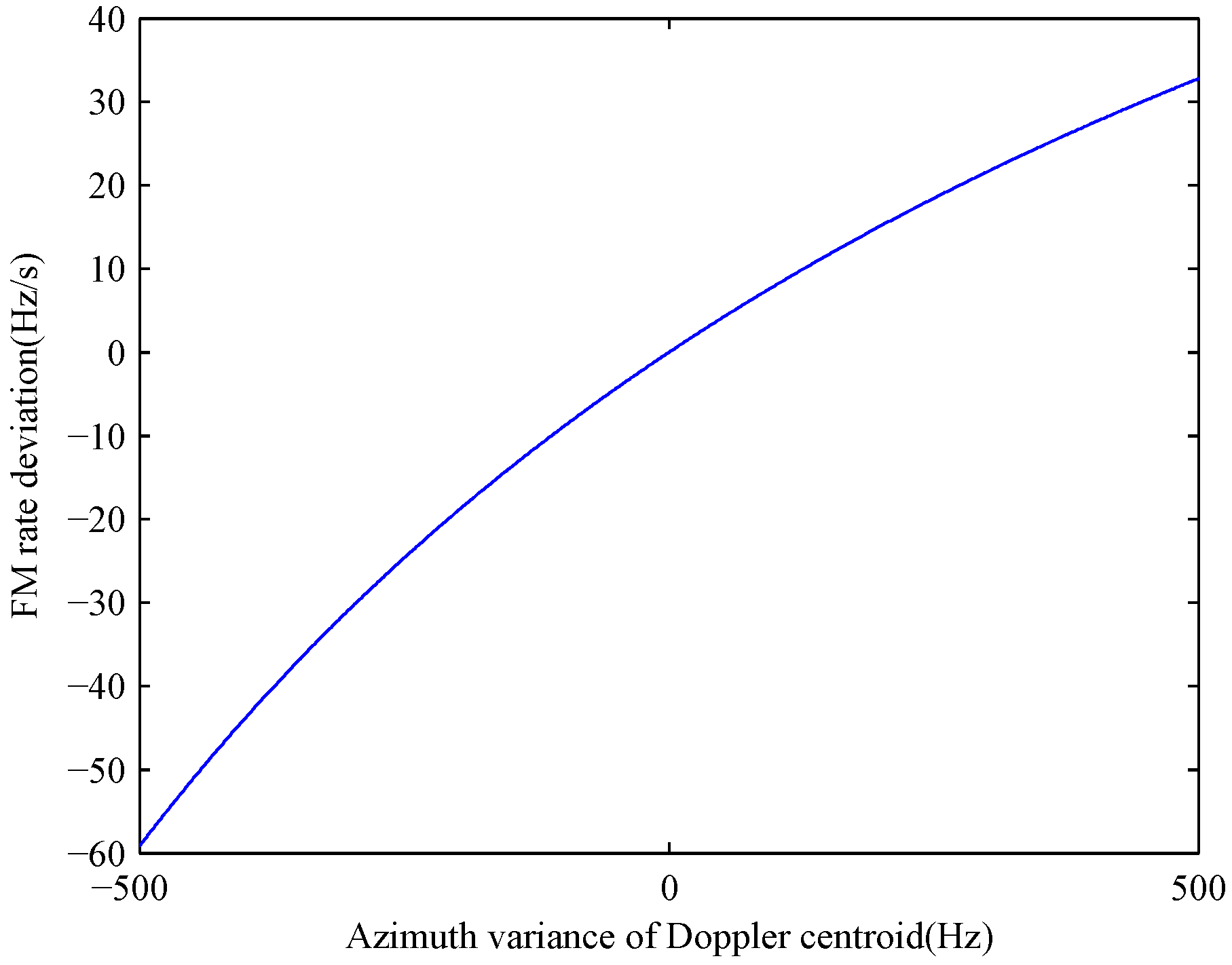
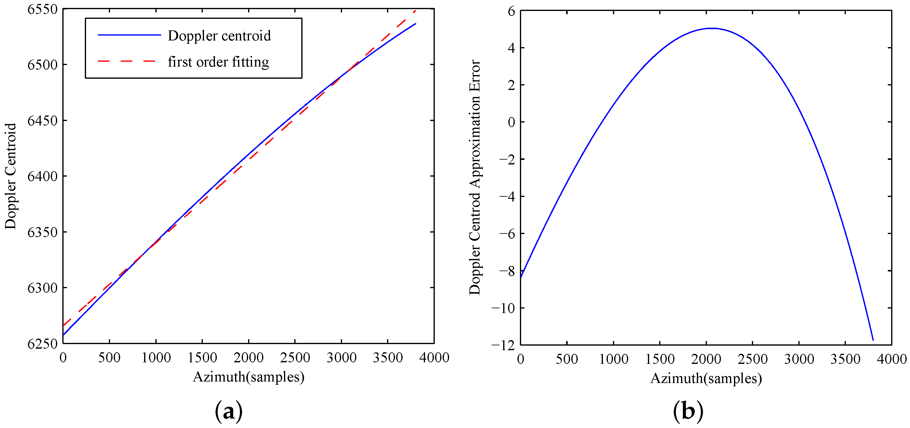
4.1. Azimuth-Dependent Doppler Coefficients Analysis

First, we expand the azimuth phase term at $t=t_R$ and keep up to the third-order term as follows:

$$\begin{array}{c}\hfill {\varphi }_{az}\left(t_m\right)=2\pi f_{dc}\left(t_m-t_R\right)+\pi f_{dr}{\left(t_m-t_R\right)}^2+\frac{\pi f_{d3}}{3}{\left(t_m-t_R\right)}^3\end{array}$$

(30)

where $f_{dc}$, $f_{dr}$, and $f_{d3}$ are the Doppler centroid, FM rate, and third-order coefficient, respectively.

Now, we shall evaluate the spatial variance of the Doppler centroid and analyze its influence on azimuth compression. $f_{dc}$ is given by

$$\begin{array}{cc}\hfill f_{dc}=& \frac{V_{R}cos{\theta }_R}{\lambda }+\frac{V_{T}cos{\theta }_T}{\lambda }\hfill \end{array}$$

(31)

where $cos{\theta }_R$ and $cos{\theta }_T$ are given by

$$\begin{array}{cc}\hfill cos{\theta }_R=& \frac{y_R}{\sqrt{x^2+y_R^2+h_R^2}}\hfill \end{array}$$

(32)

$$\begin{array}{cc}\hfill cos{\theta }_T=& \frac{sin\alpha x^{\prime }-cos\alpha y^{\prime }}{\sqrt{{x^{\prime }}^2+{y^{\prime }}^2+h_T^2}}\hfill \end{array}$$

(33)

where $x^{\prime }=x-x_T+V_{T}sin\alpha y/V_R$ and $y^{\prime }=y-y_T-V_{T}cos\alpha y/V_R$ are the contributions of the transmitter to the Doppler centroid along the cross-track direction and the azimuth direction, respectively. Inspecting Equations (31)–(33), it is obvious that the Doppler centroid of a target varies with the cross-range coordinate. First of all, generally speaking, in order to suppress the sidelobes and avoid azimuth ambiguity, the azimuth reference function undergoes a truncation operation so that its width in the time and frequency domains are both limited. If the azimuth variation of the Doppler centroid is not removed, the echo data of these targets are not in the same azimuth position in the frequency domain. Thus, some of the echo information of the targets away from the azimuth center is missed because of the reference function multiplication. The effective Doppler bandwidth is decreased, and the azimuth resolution is coarsened. The magnitudes of these targets are diminished compared with the azimuth center. When the reference function totally mismatches the echo data of the targets in the frequency domain, the targets will vanish from the scene. Moreover, if we construct the azimuth reference function using the Doppler centroid of the reference target, the imaging performance of the targets with different Doppler centroid is deteriorated. The azimuth reference function in the time domain is given by:

$$\begin{array}{c}\hfill H_{az}\left(t\right)=exp\left\{j2\pi f_{dc}t+j\pi f_{dr}{t}^2+j\frac{\pi f_{d3}}{3}{t}^3\right\}\end{array}$$

(34)

Transforming Equation (34) into the frequency domain by principle of stationary phase (POSP), the phase term is given by

$$\begin{array}{c}\hfill {\varphi }_{azcom}\left(f_a\right)=-\pi \left(\frac{f_{dc}^2}{f_{dr}}+\frac{f_{d3}{f}_{dc}^3}{3f_{dr}^3}\right)+\pi \left(\frac{2f_{dc}}{f_{dr}}+\frac{f_{d3}{f}_{dc}^2}{f_{dr}}\right)f_a-\pi \left(\frac{1}{f_{dr}}+\frac{f_{d3}{f}_{dc}}{f_{dr}^3}\right)f_a^2+\frac{\pi f_{d3}{f}_a^3}{3f_{dr}^3}\end{array}$$

(35)

The first term is a constant phase term, which should not exceed $\pi /4$. The second phase term represents first-order term of azimuth frequency, which is related to target position after azimuth compression. The third term is the second-order term of azimuth frequency, representing azimuth modulation. The last term is related to the sidelobes of the focused image. We can see from the above that the Doppler centroid influences the azimuth FM rate, first-order azimuth frequency, and the constant phase term. The spatial variation of the Doppler centroid induces a variant term into the Doppler FM rate. Thus, the Doppler FM rate is changed because of the difference of Doppler centroid between an arbitrary target and the reference target. The new FM rate is given by

$$\begin{array}{c}\hfill f_{dr}^{\prime }=\frac{1}{\left(\frac{1}{f_{dr}}+\frac{f_{d3}{f}_{dc}}{f_{dr}^3}\right)}\end{array}$$

(36)

Here, we model the azimuth dependence of the Doppler centroid as a first-order polynomial of azimuth position.

$$\begin{array}{c}\hfill f_{dc}=f_{dc0}+a{t}_R\end{array}$$

(37)

where $f_{dc0}$ is the Doppler centroid of the reference target and a is the coefficient of the first-order term of azimuth position $t_R$.

Similarly, the Doppler FM rate is modeled as a second-order polynomial of azimuth position, as follows:

$$\begin{array}{c}\hfill f_{dr}=f_{dr0}+b{t}_R+c{t}_R^2\end{array}$$

(38)

where $f_{dr0}$ is the Doppler FM rate of the reference target, and b and c are the coefficients of first-order and second-order term of azimuth position $t_R$. The quadratic and cubic phase errors induced by the approximation are given by

$$\begin{array}{c}\hfill \mathrm{\Delta }{\varphi }_{err2}=\left|\pi \left(\mathrm{\Delta }{f^{\prime }}_{dr}+\mathrm{\Delta }{f}_{dr}\right){\left(\frac{T_a}{2}\right)}^2\right|\end{array}$$

(39)

$$\begin{array}{c}\hfill \mathrm{\Delta }{\varphi }_{err3}=\left|\frac{\pi }{3}{f}_{d3}\left(\frac{1}{f_{dr}^3}-\frac{1}{{\left(f_{dr}+\mathrm{\Delta }{f^{\prime }}_{dr}+\mathrm{\Delta }{f}_{dr}\right)}^3}\right){\left(\frac{T_a}{2}\right)}^3\right|\end{array}$$

(40)

where $\mathrm{\Delta }{f}_{dr}$ is the second-order approximation error of Doppler FM rate and $\mathrm{\Delta }{f^{\prime }}_{dr}$ is

$$\begin{array}{c}\hfill \mathrm{\Delta }{f}_{dr}^{\prime }=\frac{1}{\left(\frac{1}{f_{dr}}+\frac{f_{d3}\mathrm{\Delta }{f}_{dc}}{f_{dr}^3}\right)}\end{array}$$

(41)

where $\mathrm{\Delta }{f}_{dc}$ is the first-order approximation error of the Doppler centroid.

4.2. Derivation of the Extended NLCS

In the previous subsection, the character of the spatial variation of $f_{dc}$ and $f_{dr}$ is obtained. Now, the extended NLCS is derived based on the presented analysis. Let us assume that the azimuth sampling rate is pulse repetition frequency (PRF) and the Doppler centroid of a target in a given range gate is $f_{dc}$; then, we have

$$\begin{array}{c}\hfill f_{dc}=f_{dc}^{\prime }+n\times PRF\end{array}$$

(42)

where $f_{dc}^{\prime }$ is the baseband Doppler centroid and n is the ambiguity number. If $f_{dc}^{\prime }\ne 0$, the Doppler spectrum of the target is not at the center of PRF, which is different from broadside SAR. Due to the 2-D variation of the Doppler centroid, $f_{dc}$ is different among targets in the same range gate. This difference broadens the Doppler spectrum. If $f_{dc}^{\prime }+B_a/2>PRF/2$, the echo signal is aliased, where $B_a$ is the total Doppler bandwidth. To avoid the Doppler ambiguity, an azimuth phase term is multiplied to Equation (30), which is given by

$$\begin{array}{c}\hfill H_{DC}\left(t_m\right)=exp\left\{-j2\pi f_{dc0}{t}_m\right\}\end{array}$$

(43)

After the phase multiplication, the Doppler spectrum is moved to the center of PRF, and part of the coupling term of $t_m$ and $f_{\tau }$ is removed. The azimuth phase is then given by

$$\begin{array}{c}\hfill {\varphi }_{az1}\left(t_m\right)=2\pi a{t}_R\left(t_m-t_R\right)+\pi f_{dr}{\left(t_m-t_R\right)}^2+\frac{\pi f_{d3}}{3}{\left(t_m-t_R\right)}^3\end{array}$$

(44)

First, the data after phase multiplication is transformed into the range Doppler (RD) domain. Then, a fourth-order filtering is performed

$$\begin{array}{c}\hfill H_F\left(f_a\right)=exp\left\{j\pi \left(Y_3{f}_a^3+Y_4{f}_a^4\right)\right\}\end{array}$$

(45)

where $Y_3$ and $Y_4$ are the coefficients of $H_F\left(f\right)$. The fourth-order filtering can introduce two degrees of freedom in the azimuth phase term, which are used for the derivation of the ENLCS. The azimuth phase in the frequency domain is

$$\begin{array}{c}\hfill {\varphi }_{az2}\left(f_a\right)=-2\pi f_a{t}_R-\pi \frac{{\left(f_a-a{t}_R\right)}^2}{f_{dr}}+\frac{\pi f_{d3}}{3}\frac{{\left(f_a-a{t}_R\right)}^3}{f_{dr}^3}+\pi Y_3{f}_a^3+\pi Y_4{f}_a^4\end{array}$$

(46)

Equation (46) is then transformed into the time domain:

$$\begin{array}{c}{\varphi }_{azF}\left(t_m\right)=2\pi a{t}_R\left(t_m-t_R\right)+\pi f_{dr}{\left(t_m-t_R\right)}^2\hfill \\ +\frac{\pi f_{d3}}{3}{\left(t_m-t_R\right)}^3+\pi Y_3{[f_{dr}(t_m-t_R)+a{t}_R]}^3+\pi Y_4{[f_{dr}(t_m-t_R)+a{t}_R]}^4\hfill \end{array}$$

(47)

After the fourth-order filtering, an azimuth NLCS factor is introduced to equalize the spatially-variant Doppler centroid as well as the FM rate. The NLCS factor is given as follows:

$$\begin{array}{c}\hfill H_{NLCS}\left(t_m\right)=exp\left\{j\pi (q_2{t}_m^2+q_3{t}_m^3+q_4{t}_m^4)\right\}\end{array}$$

(48)

where $q_2$, $q_3$, and $q_4$ are the coefficients of the NLCS operator. The azimuth phase in the time domain after fourth-order filtering is then multiplied by the NLCS factor and transformed into the frequency domain:

$$\begin{array}{cc}\hfill {\varphi }_{azNLCS}\left(f_a\right)=& \pi \frac{-a^2-2a{q}_2+f_{dr}{q}_2}{q_2+f_{dr}}{t}_R^2+\frac{2\pi \left(a-f_{dr}\right)}{q_2+f_{dr}}{f}_a-\frac{\pi f_a^2}{q_2+f_{dr}}+\frac{\pi }{3}{f}_{d3}\frac{{\left[f_a-\left(a+q_2\right)t_R\right]}^3}{{\left(q_2+f_{dr}\right)}^3}\hfill \\ & +\pi Y_3\frac{{\left[f_{dr}{f}_a-\left(f_{dr}-a\right)q_2{t}_R\right]}^3}{{\left(q_2+f_{dr}\right)}^3}+\pi Y_4\frac{{\left[f_{dr}{f}_a-\left(f_{dr}-a\right)q_2{t}_R\right]}^4}{{\left(q_2+f_{dr}\right)}^4}\hfill \\ & +\pi q_3\frac{{\left[f_a-\left(a-f_{dr}\right)t_R\right]}^3}{{\left(q_2+f_{dr}\right)}^3}+\pi q_4\frac{{\left[f_a-\left(a-f_{dr}\right)t_R\right]}^4}{{\left(q_2+f_{dr}\right)}^4}\hfill \end{array}$$

(49)

Using the approximation presented in Equations (37) and (38), we expand the above phase term into a power series of $t_R$ and $f_a$

$$\begin{array}{c}\hfill {\varphi }_{azNLCS}\left(f_a\right)\approx D\left(f_a\right)+E{t}_R{f}_a+F{t}_R^2{f}_a+G{t}_R{f}_a^2+H{t}_R^2{f}_a^2+I{t}_R{f}_a^3+J\left(t_R\right)\end{array}$$

(50)

where E, F, G, H, and I are the expanding coefficients of the coupling term of $t_R$ and $f_a$, which are given in Equation (51). Inspecting Equation (50), the first term $D\left(f_a\right)$ represents the azimuth modulation term, which is independent of azimuth position. The second term is the azimuth position of the targets after compression. The third term causes a nonlinear shift of azimuth position. The fourth and fifth terms represent the spatial variation of Doppler FM rate along the azimuth direction. The sixth term is the spatial variation of the third-order coefficient of Doppler frequency, which influences the sidelobes of the target after azimuth compression. The seventh term is independent of azimuth frequency, and can be neglected.

$$\begin{array}{c}\hfill E=\frac{2\pi \left(a-f_{dr0}\right)}{q_2+f_{dr0}}\end{array}$$

(51)

$$\begin{array}{c}\hfill F=-\frac{2\pi b\left(q_2-a\right)}{{\left(q_2+f_{dr0}\right)}^2}+\pi f_{d3}\frac{{\left(a+q_2\right)}^2}{{\left(q_2+f_{dr0}\right)}^3}+3\pi Y_3\frac{{\left(f_{dr0}-a\right)}^2{q}_2^2{f}_{dr0}}{{\left(q_2+f_{dr0}\right)}^3}+3\pi q_3\frac{{\left(a-f_{dr0}\right)}^2}{{\left(q_2+f_{dr0}\right)}^3}\end{array}$$

(52)

$$\begin{array}{c}\hfill G=\frac{\pi b}{{\left(q_2+f_{dr0}\right)}^2}-\pi f_{d3}\frac{\left(a+q_2\right)}{{\left(q_2+f_{dr0}\right)}^3}-3\pi Y_3\frac{\left(f_{dr0}-a\right)q_2{f}_{dr0}^2}{{\left(q_2+f_{dr0}\right)}^3}-3\pi q_3\frac{\left(a-f_{dr0}\right)}{{\left(q_2+f_{dr0}\right)}^3}\end{array}$$

(53)

$$\begin{array}{cc}\hfill H=& \pi \frac{c\left(q_2+f_{dr0}\right)-b^2}{{\left(q_2+f_{dr0}\right)}^3}+3\pi f_{d3}\frac{b\left(a+q_2\right)}{{\left(q_2+f_{dr0}\right)}^4}-3\pi Y_3{q}_2\frac{b{f}_{dr0}\left(3f_{dr0}{q}_2-2a{q}_2+f_{dr0}a\right)}{{\left(q_2+f_{dr0}\right)}^4}\hfill \\ & +\pi Y_4\frac{6f_{dr0}^2\left(f_{dr0}-a\right)q_2^2}{{\left(q_2+f_{dr0}\right)}^4}+3\pi q_3\frac{b\left(q_2+3a-2f_{dr0}\right)}{{\left(q_2+f_{dr0}\right)}^4}+6\pi q_4\frac{{\left(a-f_{dr0}\right)}^2}{{\left(q_2+f_{dr0}\right)}^4}\hfill \end{array}$$

(54)

$$\begin{array}{cc}\hfill I=& -\frac{\pi f_{d3}b}{{\left(q_2+f_{dr0}\right)}^4}+3\pi Y_3\frac{b{f}_{dr0}^2{q}_2}{{\left(q_2+f_{dr0}\right)}^4}-4\pi Y_4\frac{f_{dr0}^3\left(f_{dr0}-a\right)q_2}{{\left(q_2+f_{dr0}\right)}^4}\hfill \\ & -3\pi q_3\frac{b}{{\left(q_2+f_{dr0}\right)}^4}-4\pi q_4\frac{\left(a-f_{dr0}\right)}{{\left(q_2+f_{dr0}\right)}^4}\hfill \end{array}$$

(55)

In order to eliminate the azimuth variation of Doppler coefficients, the coefficient of the first-order coupling of $f_a$ and $t_R$ is set to $-\pi /\beta$, where β is a constant scaling factor which determines the azimuth position of the targets. Furthermore, the coefficients of other coupling terms is set to zero. Thus, we obtain an equation system with five unknowns:

$$\begin{array}{c}\hfill \left\{\begin{array}{c}E=-\pi /\beta \hfill \\ F=0\hfill \\ G=0\hfill \\ H=0\hfill \\ I=0\hfill \end{array}\right.\end{array}$$

(56)

Solving Equation (56), the parameters of fourth-order filtering and NLCS are given by

$$\begin{array}{c}\hfill q_2=-2a\beta +\left(2\beta -1\right)f_{dr0}\end{array}$$

(57)

$$\begin{array}{c}\hfill Y_3=\frac{b\left(2q_2+a+f_{dr0}\right)-f_{d3}\left(a+q_2\right)}{3{\left(f_{dr0}-a\right)}^2{q}_2{f}_{dr0}}\end{array}$$

(58)

$$\begin{array}{c}\hfill q_3=\frac{2b\left(q_2+a\right)\left(q_2+f_{dr0}\right)-f_{d3}{\left(a+q_2\right)}^2-q_{2}N}{3{\left(f_{dr0}-a\right)}^2}\end{array}$$

(59)

$$\begin{array}{cc}\hfill Y_4=& \frac{L/6-M\left(a-f_{dr0}\right)/4}{{\left(f_{dr0}-a\right)}^2{q}_2{f}_{dr0}^2\left(q_2+f_{dr0}\right)}\hfill \end{array}$$

(60)

$$\begin{array}{cc}\hfill q_4=& \frac{M/4-\left(f_{dr0}-a\right)f_{dr0}^3{q}_2{Y}_4}{a-f_{dr0}}\hfill \end{array}$$

(61)

where L, M, and N are given in Equations (62)–(64).

$$\begin{array}{c}\hfill N=b\left(2q_2+a+f_{dr0}\right)-f_{d3}\left(a+q_2\right)\end{array}$$

(62)

$$\begin{array}{cc}\hfill L=& -\left[c{\left(q_2+f_{dr0}\right)}^2-b^2\left(q_2+f_{dr0}\right)\right]-3f_{d3}b\left(a+q_2\right)-3q_{3}b\left(q_2-2f_{dr0}+3a\right)\hfill \\ & +3Y_3{q}_{2}b{f}_{dr0}\left(3f_{dr0}{q}_2-2a{q}_2+f_{dr0}a\right)\hfill \end{array}$$

(63)

$$\begin{array}{cc}\hfill M=& -3f_{d3}b+3Y_3{q}_{2}b{f}_{dr0}^2-3q_{3}b\hfill \end{array}$$

(64)

After the fourth-order filtering and NLCS process, the phase of the echo signal in the frequency domain is given by

$$\begin{array}{c}\hfill {\varphi }_{az3}\left(f_a\right)=-\frac{\pi }{\beta }{t}_R{f}_a-\frac{\pi f_a^2}{q_2+f_{dr0}}+\pi \frac{\left(f_{d3}/3+Y_3{f}_{dr0}^3+q_3\right)f_a^3}{{\left(q_2+f_{dr0}\right)}^3}+\pi \frac{\left(Y_4{f}_{dr0}^4+q_4\right)f_a^4}{{\left(q_2+f_{dr0}\right)}^4}\end{array}$$

(65)

It is obvious that in Equation (65), the spatial variance of the Doppler centroid and the FM rate is removed.

The Doppler coefficients of all the targets in the same range gate are processed to be the same. Notice that the azimuth FM rate after the process is changed to $f_{drnew}=q_2+f_{dr0}$. When β equals $0.5$, the target after azimuth compression is at its real position. While β is larger than $0.5$, the azimuth distance among targets in the same range gate is enlarged. However, β cannot be too far from $0.5$, because the larger β is, the larger is the absolute value of $f_{drnew}$. Additionally, the Doppler bandwidth is widened, which may cause azimuth aliasing. On the other hand, β should not be too small, because the targets may get too close to each other. Thus, β is better chosen to be $0.5$. Figure 3 shows the Doppler spectra of the simulated targets before and after the extended NLCS operation. It is clear that before extended NLCS, the Doppler spectra of different targets are located at different azimuth positions, due to 2-D variance of the Doppler centroid. After the extended NLCS operation, the Doppler spectra of all targets are moved to the center of the azimuth frequency, and the azimuth variation of the Doppler centroid is removed with respect to every range gate. The Doppler bandwidth of the three range gates 3350, 4096, and 4950 are 215.53 Hz, 228.85 Hz, and 240.14 Hz, respectively. This phenomenon is due to their differences in azimuth processing. The coefficients of fourth-order filtering, NLCS, and the azimuth compression factor are calculated with respect to every range gate. Thus, the Doppler FM rates of the targets after azimuth NLCS are slightly different from each other.

According to Equation (65), the azimuth compression function is given by

$$H_{AC}\left(f_a\right)=exp\left\{\frac{\pi f_a^2}{q_2+f_{dr0}}\right\}\times exp\left\{-\pi \frac{\left(f_{d3}/3+Y_3{f}_{dr0}^3+q_3\right)f_a^3}{{\left(q_2+f_{dr0}\right)}^3}\right\}\times exp\left\{-\pi \frac{\left(Y_4{f}_{dr0}^4+q_4\right)f_a^4}{{\left(q_2+f_{dr0}\right)}^4}\right\}$$

(66)

Figure 4 shows the flowchart of the proposed algorithm.

In the derivation of the proposed algorithm, the azimuth dependence of the Doppler centroid and FM rate are approximated by a first-order polynomial function and a second-order polynomial function, respectively. Moreover, the spatial variation of the third-order Doppler coefficient is neglected. Based on the analysis in this paper, the approximations here are valid, and the corresponding errors are small enough that we can ignore them. However, these approximations can cause some errors in specific geometry configurations where the azimuth dependence of the Doppler character is more complicated, and the order of the polynomial function chosen in this paper is not enough. In addition, if we ignore the spatial variance of the third-order Doppler coefficient, the corresponding phase error may be larger than $\pi /4$, and it will influence the azimuth compression performance. Thus, the imaging quality can get worse. In such cases, we can increase the order of approximation of the polynomial function and take the spatial variance of third-order Doppler coefficient into consideration, but it will make the derivation much more complex.

4.3. Computation Complexity

From the above analysis, the proposed imaging algorithm includes two instances of range FFT and inverse FFT (IFFT) and four instances of azimuth FFT and IFFT. The major operations include a keystone transform and five instances of 2-D phase factor multiplication; i.e., range compression, second order RCMC, fourth order filtering, extended NLCS, and azimuth compression. Suppose that the range sample number is denoted as $N_r$ and the azimuth sample number is $N_a$. The total number of real floating-point operations is

$$\begin{array}{c}\hfill 10N_r{N}_a{log}_2\left(N_r\right)+20N_r{N}_a{log}_2\left(N_a\right)+30N_r{N}_a+2\left(2M_{ker}-1\right)N_r{N}_a\end{array}$$

(67)

where $M_{ker}$ is the number of neighbor samples used for the range and azimuth interpolation. Therefore, the computational complexity is of order $O\left(N^2{log}_{2}N\right)$, where N is the 1-D size of the data. It can be concluded that the computation complexity of the proposed method is of the same order as traditional range Doppler algorithm (RDA) and $\omega KA$ and more efficient than back-projection, whose computation complexity is of order $O\left(N^3\right)$.

5. Simulation and Real Data Processing Results

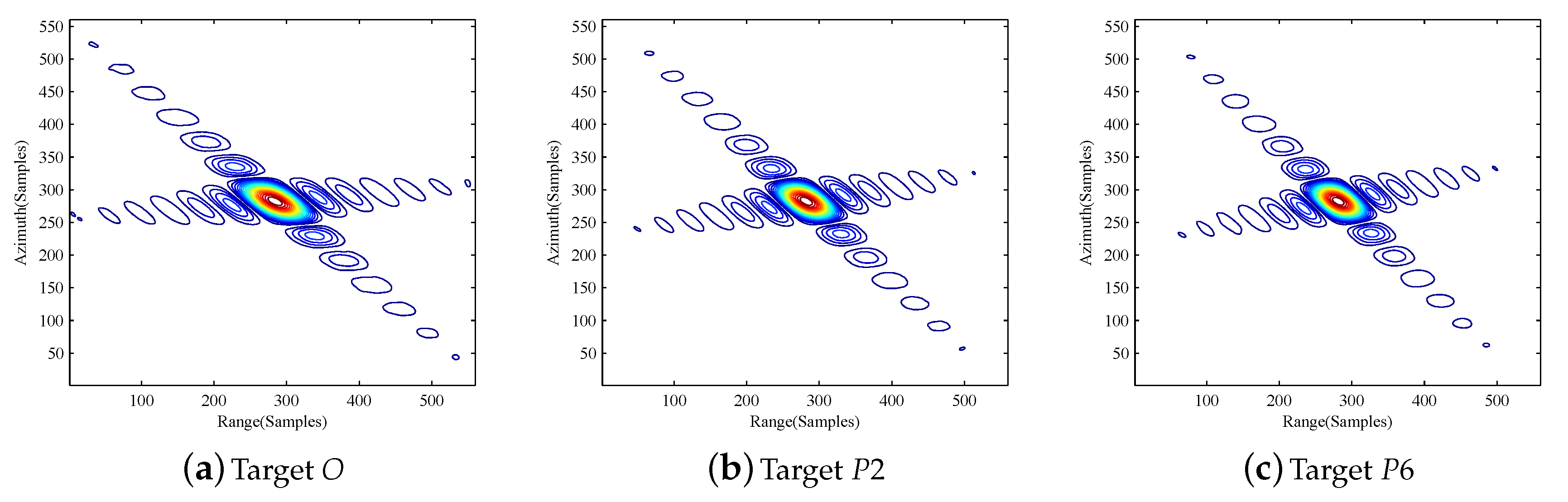
5.1. Numerical Simulation Verification

Numerical simulations are carried out in this subsection to verify the effectiveness of the proposed imaging algorithm. The simulation parameters are listed in

Table 1. Simulation parameters.

Parameter	Transmitter	Receiver
Original Position	(−8000, −1000, 6000) m	(0,−6000, 4000) m
Velocity	100 m/s	300 m/s
Trajectory Angle	45 degree
Carrier Frequency	9.6 GHz
Range Bandwidth	200 MHz
Pulse Repetition Frequency	1000 Hz
Synthetic Aperture Time	1 s

.

The receiver can be mounted on a fighter. In the following simulation, the locations of the 12 targets are shown in Figure 5. The azimuth distance between targets $P1$–$P6$ and scene center O are 350 m, and the azimuth distance between targets $P7$–$P12$ and the scene center are 175 m. The coordinates of targets $P1$–$P6$ are $(-54.6576,350)$ m, $(-443.4703,350)$ m, $(-872.9143,350)$ m, $(707.1249,-350)$ m, $(381.2807,-350)$ m, and $(32.1523,-350)$ m, respectively. Targets $P7$–$P12$ are the mid-points on the lines of $P1$–$P6$ and scene center O. The positions of the targets are chosen in this way so that targets $P1$ and $P4$, $P2$, O, and $P5$, $P3$, and $P6$ are in the same range gates after KT and higher-order RCMC, respectively. Thus, we can evaluate the effectiveness of the algorithm both in the azimuth and range directions.

First of all, the expanding coefficients $A_R$, $B_R$, $C_R$, and $A_T$, $B_T$, $C_T$ in the simulated case are 249.6151 m/s, 3.8402 m/s${}^2$, 0.3988 m/s${}^3$, and $-49.2518$ m/s, 0.7537 m/s${}^2$, and −0.0111 m/s${}^3$, respectively. It can be seen that $A_{R,T}$ is much larger than $B_{R,T}$ and $C_{R,T}$, and LRCM is the most significant in bistatic forward-looking SAR.

Figure 6 shows the residual RCM of the three simulated targets and their corresponding spatial variance. It can be seen that the residual RCMs of the simulated targets are approximately 10 m with 2 s synthetic aperture time. The residual RCMs exceed one resolution cell and should be compensated. However, the spatial variance of residual RCM between the targets is 0.1 m, which is smaller than one resolution cell and can be ignored.

Figure 7 shows the echo of the seven simulated targets (targets O and $P1$–$P6$) before and after the higher-order RCMC operation. We can find that in Figure 7a,c, the energy of a single target is spread across multiple range gates due to higher-order RCM. In Figure 7b,d, this problem is solved and the energy is gathered in one range gate.

Figure 8 shows the Doppler FM rate deviation induced by the azimuth variation of the Doppler centroid according to Equation (41). Figure 8 illustrates that FM rate varies considerably when the Doppler centroid changes, and it has a great influence on the azimuth focusing. A variance of 500 Hz in the Doppler centroid can cause a FM rate deviation of 30 Hz/s. If the problem of spatial variation of the Doppler centroid is not settled properly, only the reference target can be well-focused, and the imaging quality of the rest of the targets suffer great degradation.

Figure 9 and Figure 10 show the first-order fitting of the Doppler centroid and the second-order fitting of FM rate, and their corresponding approximation errors, respectively. It can be seen that $\mathrm{\Delta }{\varphi }_{err2}$ and $\mathrm{\Delta }{\varphi }_{err3}$ are less than $\pi /4$. Thus, the first-order and second-order approximations of the Doppler centroid and FM rate are precise enough, respectively. The approximation errors are small enough that we can ignore their impacts on azimuth compression.

Figure 11 shows the imaging results of the simulated targets in the scene. The results are interpolated by adding zeros in the frequency domain and transforming back to the time domain. All of the targets are well-focused by the proposed imaging algorithm. We can find that the aforementioned targets are gathered in the same range gates, and the azimuth positions of the targets are not changed by the processing because β is chosen to be 0.5 in this simulation.

Figure 12 and Figure 13 show the detailed imaging results of targets O, $P2$, $P6$, $P7$, $P9$, and $P11$. The results of the proposed method are compared with two state-of-the-art methods—i.e., the traditional NLCS method of Qiu et al. [34] and the fast backprojection (FBP) method. In the traditional azimuth NLCS method, the spatial variation of the Doppler FM rate is first obtained by local curve fitting, and the azimuth perturbation function is then derived by numerical integration. However, this ignores the azimuth variation of the Doppler centroid, and the FM rate deviation induced by it is not removed by the NLCS process. Thus, after the traditional NLCS process, the Doppler FM rates of the targets in the same range gate are still not equalized. Inspecting Figure 12g–l, it is clear that only the azimuth scene center is well-focused, and the azimuth compression performance of other targets suffer great degradation because the Doppler FM rates are still different from each other. In the upper two rows, the Doppler centroid and the FM rates are both equalized by the extended NLCS algorithm. Thus, when multiplied by the same azimuth compression factor, all of the targets get well focused. On the other hand, comparing the imaging results of the proposed method with that of the FBP method in Figure 13, it can be seen that the focusing performance of our method is close to the FBP method. However, the FBP method has more computational complexity than the proposed method, which is the drawback of time-domain imaging methods. The measured parameters peak sidelobe ratio (PSLR) and integrated sidelobe ratio (ISLR) of targets $P2$, $P5$, $P6$, $P7$, $P9$, and $P11$ are listed in

Table 2. Measured parameters of the selected targets. PSLR: peak sidelobe ratio; ISLR: integrated sidelobe ratio; FBP: fast backprojection.

	Targets	Azimuth		Range
		PSLR (dB)	ISLR (dB)	PSLR (dB)	ISLR (dB)
Proposed Algorithm	P2	−12.86	−9.86	−13.02	−9.73
	P5	−12.34	−9.74	−13.16	−9.96
	P6	−13.07	−9.87	−12.86	−9.36
	P7	−12.74	−9.73	−13.11	−9.77
	P9	−12.48	−9.48	−12.74	−9.73
	P11	−12.50	−9.88	−13.06	−9.44
Qiu’s Method	P2	N/A	N/A	−13.33	−8.71
	P5	N/A	N/A	−12.76	−9.03
	P6	N/A	N/A	−12.58	−7.96
	P7	−5.23	−5.74	−13.04	−9.04
	P9	−7.58	−7.65	−12.88	−8.84
	P11	−6.70	−7.22	−12.56	−8.56
FBP Method	P2	−12.67	−9.96	−13.21	−9.63
	P5	−13.36	−9.73	−13.32	−9.73
	P6	−12.95	−9.57	−12.67	−9.80
	P7	−13.21	−9.73	−13.01	−9.87
	P9	−12.66	−9.45	−13.04	−9.63
	P11	−13.08	−9.87	−13.06	−9.91

. The PLSR and ISLR of the imaging results of the proposed are around $-13$ dB and $-10$ dB, which are nearly theoretical values. However, the parameters of the NLCS algorithm are worse compared to the proposed algorithm in the azimuth direction.

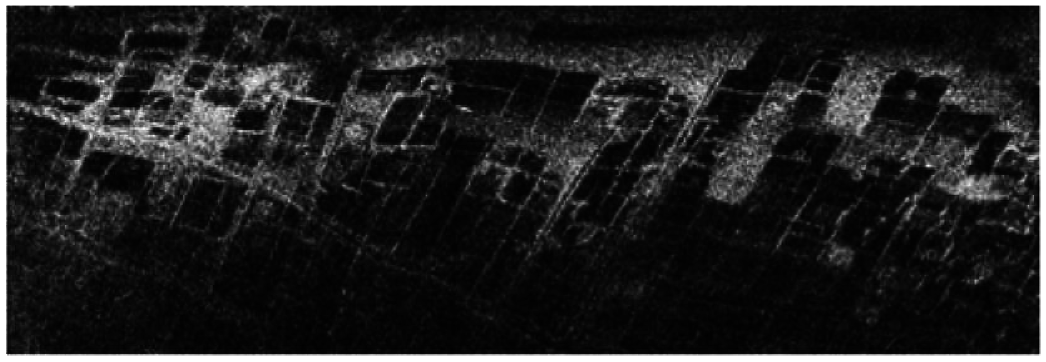
5.2. Real Data Processing Results

In order to further verify the effectiveness of the proposed method, real airborne bistatic SAR data processing results are given in Figure 14, and comparison between the traditional NLCS method of Qiu in Figure 15 et al. [34] is made in this subsection. The bistatic SAR system works in the X band with 75 MHz chirp bandwidth. The pulse repetition frequency is 500 Hz, and the pulse width is 20 $\mathsf{\mu }$s. The velocity is 42 m/s, and the flying height for the transmitter and the receiver are 800 m and 600 m, respectively.

6. Discussion

Based on the results and analysis in Section 5, it can be concluded that the proposed algorithm can achieve accurate focusing for TV-BFSAR data. The main problems for TV-BFSAR imaging are 2-D spatial variant RCM and azimuth variant Doppler parameters (i.e., Doppler centroid and FM rate). For the first problem, the proposed RCMC method using keystone transform and higher-order RCM correction can remove the spatially-variant RCM of all the targets precisely compared with current methods, such as linear range walk correction (LRWC). On the other hand, the extended azimuth NLCS can equalize the azimuth variant Doppler centroid as well as FM rate, which obtains better azimuth focusing performance than the traditional NLCS method.

It should be noted that the ancillary data (such as Tx and Rx position, velocity, and attitude) should be accurate enough for the application of the method. These data can be either obtained by GPS and attitude instrument or by autofocus techniques [35,36,37]. Here we assume that the ancillary data are derived from GPS and attitude instrument onboard the Tx and Rx and are accurate enough for the processing method. Moreover, if motion error exists for the transmitting and receiving platforms, motion compensation should be utilized to obtain satisfactory imaging results. Autofocus techniques can be integrated in the proposed method to estimate the ancillary parameters and further improve the focusing performance, which is our future work.

7. Conclusions

In this paper, an imaging algorithm for translational-variant bistatic forwarding SAR is proposed. The algorithm can be grouped into two parts: the range RCMC and azimuth extended NLCS. The range RCMC mainly deals with the problem of the spatial variation of first-order RCM and the residual higher-order RCM. The extended NLCS equalizes the Doppler centroid as well as FM rate. The range RCMC procedures are as follows. First, Keystone Transform is performed on the echo signal to remove the spatially-variant linear RCM. Second, the echo signal is compressed using a new range FM rate. Third, a correction factor is multiplied to the echo data to compensate for the higher-order RCM. Then, the azimuth dependence of the Doppler characters is calculated based on the relationship of cross-range coordinate x with azimuth position y and slant range R. The azimuth processing can also be divided into three parts. First, a phase factor is multiplied to the echo to move the Doppler spectra of the reference targets to the center of the azimuth frequency with respect to every range gate. Second, a fourth-order filtering is performed, which can introduce two degrees of freedom in the azimuth phase term. Third, an azimuth NLCS operation is carried out to equalize the azimuth-variant Doppler centroid and FM rate. At last, the targets in the same range gate are compressed by the same reference function.

Verified by the simulated and real TV-BFSAR data, this algorithm resolves the problem of the variation of both Doppler centroid and linear RCM, and thus has higher accuracy for all the targets in the scene. The residual RCM after keystone transform and higher-order RCMC is less than one resolution cell, which is accurate enough for TV-BFSAR imaging. The proposed method can achieve accurate focusing of TV-BFSAR data compared with tradition NLCS methods. The PSLR and ISLR of the simulated target are approximately −13 dB and −10 dB. Last but not least, the proposed method is more efficient than the backprojection method.

References

1. Yu, Z.; Wang, S.; Li, Z. An imaging compensation algorithm for spaceborne high-resolution SAR based on a continuous tangent motion model. Remote Sens. 2016, 8, 223. [Google Scholar] [CrossRef]
2. Huang, P.; Xu, W. A new spaceborne burst synthetic aperture radar imaging mode for wide swath coverage. Remote Sens. 2014, 6, 801. [Google Scholar] [CrossRef]
3. Perna, S.; Esposito, C.; Amaral, T.; Berardino, P.; Jackson, G.; Moreira, J.; Pauciullo, A.; Vaz Junior, E.; Wimmer, C.; Lanari, R. The InSAeS4 airborne X-band interferometric SAR system: A first assessment on its imaging and topographic mapping capabilities. Remote Sens. 2016, 8, 40. [Google Scholar] [CrossRef]
4. Raspini, F.; Ciampalini, A.; Del Conte, S.; Lombardi, L.; Nocentini, M.; Gigli, G.; Ferretti, A.; Casagli, N. Exploitation of amplitude and phase of satellite SAR images for landslide mapping: The case of Montescaglioso (South Italy). Remote Sens. 2015, 7, 14576. [Google Scholar] [CrossRef]
5. Curlander, J.C.; McDonough, R.N. Synthetic Aperture Radar: Systems and Signal Processing; Wiley: New York, NY, USA, 1991; Volume 199. [Google Scholar]
6. Walterscheid, I.; Klare, J.; Brenner, A.R.; Ender, J.H.; Loffeld, O. Challenges of a bistatic spaceborne/airborne SAR experiment. In Proceedings of the 6th European Conference on Synthetic Aperture Radar (EUSAR 2006), Dresden, Germany, 16–18 May 2006.
7. Wu, J.; Yang, J.; Huang, Y.; Yang, H.; Wang, H. Bistatic forward-looking SAR: Theory and challenges. In Proceedings of the 2009 IEEE Radar Conference, Pasadena, CA, USA, 4–8 May 2009; pp. 1–4.
8. Li, W.; Huang, Y.; Yang, J.; Wu, J.; Kong, L. An improved Radon-transform-based scheme of doppler centroid estimation for bistatic forward-looking SAR. IEEE Geosci. Remote Sens. Lett. 2011, 8, 379–383. [Google Scholar] [CrossRef]
9. Walterscheid, I.; Espeter, T.; Klare, J.; Brenner, A.R.; Ender, J.H. Potential and limitations of forward-looking bistatic SAR. In Proceedings of the 2010 IEEE International Geoscience and Remote Sensing Symposium (IGARSS), Honolulu, HI, USA, 25–30 July 2010; pp. 216–219.
10. Qiu, X.; Hu, D.; Ding, C. Some reflections on bistatic SAR of forward-looking configuration. IEEE Geosci. Remote Sens. Lett. 2008, 5, 735–739. [Google Scholar] [CrossRef]
11. Wu, J.; Yang, J.; Huang, Y.; Yang, H. A frequency-domain imaging algorithm for translational invariant bistatic forward-looking SAR. IEICE Trans. Commun. 2013, 96, 605–612. [Google Scholar] [CrossRef]
12. Wang, R.; Loffeld, O.; Nies, H.; Peters, V. Image formation algorithm for bistatic forward-looking SAR. In Proceedings of the 2010 IEEE International Geoscience and Remote Sensing Symposium (IGARSS), Honolulu, HI, USA, 25–30 July 2010; pp. 4091–4094.
13. Hu, C.; Long, T.; Zeng, T.; Yang, C. Forward-looking bistatic SAR range migration alogrithm. In Proceedings of the International IEEE Conference on Radar (CIE’06), Shanghai, China, 16–19 October 2006; pp. 1–4.
14. Shin, H.S.; Lim, J.T. Omega-k algorithm for airborne forward-looking bistatic spotlight SAR imaging. IEEE Geosci. Remote Sens. Lett. 2009, 6, 312–316. [Google Scholar] [CrossRef]
15. Zeng, D.; Zeng, T.; Hu, C.; Long, T. Back-projection algorithm characteristic analysis in forward-looking bistatic SAR. In Proceedings of the International IEEE Conference on Radar (CIE’06), Shanghai, China, 16–19 October 2006; pp. 1–4.
16. Qiu, X.; Behner, F.; Reuter, S.; Nies, H.; Loffeld, O.; Huang, L.; Hu, D.; Ding, C. An imaging algorithm based on keystone transform for one-stationary bistatic SAR of spotlight mode. J. Adv. Signal Process. 2012, 2012, 352–356. [Google Scholar] [CrossRef]
17. Walterscheid, I.; Brenner, A.R.; Klare, J. Radar imaging with very low grazing angles in a bistatic forward-looking configuration. In Proceedings of the 2012 IEEE International Geoscience and Remote Sensing Symposium (IGARSS), Munich, Germany, 22–27 July 2012; pp. 327–330.
18. Wu, J.; Huang, Y.; Yang, J.; Li, W.; Yang, H. First result of bistatic forward-looking SAR with stationary transmitter. In Proceedings of the 2011 IEEE International Geoscience and Remote Sensing Symposium (IGARSS), Vancouver, BC, Canada, 24–29 July 2011; pp. 1223–1226.
19. Yang, J.; Huang, Y.; Wu, J.; Li, W.; Li, Z.; Yang, X. A first experiment of airborne bistatic forward-looking SAR-preliminary results. In Proceedings of the 2013 IEEE International Geoscience and Remote Sensing Symposium (IGARSS), Melbourne, Australia, 21–26 July 2013.
20. Shao, Y.F.; Wang, R.; Deng, Y.K.; Liu, Y. Digital elevation model reconstruction in multichannel spaceborne/stationary SAR interferometry. IEEE Geosci. Remote Sens. Lett. 2014, 11, 2080–2084. [Google Scholar] [CrossRef]
21. Anghel, A.; Cacoveanu, R.; Moldovan, A.-S.; Popescu, A.-A.; Datcu, M.; Serban, F. Simplified bistatic SAR imaging with a fixed receiver and TerraSAR-X as transmitter of opportunity—First results. In Proceedings of the 2016 IEEE International Geoscience and Remote Sensing Symposium (IGARSS), Beijing, China, 10–15 July 2016.
22. Wu, J.; Li, Z.; Huang, Y.; Yang, J.; Liu, Q. A generalized omega-k algorithm to process translationally variant bistatic SAR data based on two-dimensional stolt mapping. IEEE Trans. Geosci. Remote Sens. 2014, 52, 6597–6614. [Google Scholar]
23. Wong, F.; Yeo, T.S. New applications of nonlinear chirp scaling in SAR data processing. IEEE Trans. Geosci. Remote Sens. 2001, 39, 946–953. [Google Scholar] [CrossRef]
24. An, D.; Huang, X.; Jin, T.; Zhou, Z. Extended nonlinear chirp scaling algorithm for high-resolution highly squint SAR data focusing. IEEE Trans. Geosci. Remote Sens. 2012, 50, 3595–3609. [Google Scholar] [CrossRef]
25. Sun, G.; Jiang, X.; Xing, M.; Qiao, Z.j.; Wu, Y.; Bao, Z. Focus improvement of highly squinted data based on azimuth nonlinear scaling. IEEE Trans. Geosci. Remote Sens. 2011, 49, 2308–2322. [Google Scholar] [CrossRef]
26. Perry, R.; Dipietro, R.; Fante, R. SAR imaging of moving targets. IEEE Trans. Aerosp. Electron. Syst. 1999, 35, 188–200. [Google Scholar] [CrossRef]
27. Zhou, F.; Wu, R.; Xing, M.; Bao, Z. Approach for single channel SAR ground moving target imaging and motion parameter estimation. IET Radar Sonar Navig. 2007, 1, 59–66. [Google Scholar] [CrossRef]
28. Wu, J.; Li, Z.; Huang, Y.; Yang, J.; Yang, H.; Liu, Q. Focusing bistatic forward-looking SAR with stationary transmitter based on keystone transform and nonlinear chirp scaling. IEEE Geosci. Remote Sens. Lett. 2014, 11, 148–152. [Google Scholar] [CrossRef]
29. Li, Z.; Wu, J.; Li, W.; Huang, Y.; Yang, J. One-stationary bistatic side-looking SAR imaging algorithm based on extended keystone transforms and nonlinear chirp scaling. IEEE Geosci. Remote Sens. Lett. 2013, 10, 211–215. [Google Scholar]
30. Dai, C.; Zhang, X. Bistatic SAR image formation algorithm using keystone transform. In Proceedings of the IEEE Radar Conference (RADAR), Kansas City, MO, USA, 23–27 May 2011; pp. 342–345.
31. Zhong, H.; Liu, X. An extended nonlinear chirp-scaling algorithm for focusing large-baseline azimuth-invariant bistatic SAR data. IEEE Geosci. Remote Sens. Lett. 2009, 6, 548–552. [Google Scholar] [CrossRef]
32. Wong, F.H.; Cumming, I.G.; Neo, Y.L. Focusing bistatic SAR data using the nonlinear chirp scaling algorithm. IEEE Trans. Geosci. Remote Sens. 2008, 46, 2493–2505. [Google Scholar] [CrossRef]
33. Liu, G.G.; Zhang, L.R.; Liu, X. General bistatic SAR data processing based on extended nonlinear chirp scaling. IEEE Trans. Geosci. Remote Sens. 2013, 10, 976–980. [Google Scholar]
34. Qiu, X.; Hu, D.; Ding, C. An improved NLCS algorithm with capability analysis for one-stationary BiSAR. IEEE Trans. Geosci. Remote Sens. 2008, 46, 3179–3186. [Google Scholar] [CrossRef]
35. Zhang, L.; Sheng, J.; Xing, M.; Qiao, Z.; Xiong, T.; Bao, Z. Wavenumber-domain autofocusing for highly squinted UAV SAR imagery. IEEE Sens. J. 2012, 12, 1574–1588. [Google Scholar] [CrossRef]
36. Zhang, L.; Wang, G.; Qiao, Z.; Wang, H. Azimuth motion compensation with improved subaperture algorithm for airborne SAR imaging. IEEE J. Sel. Top. Appl. Earth Observ. Remote Sens. 2016. [Google Scholar] [CrossRef]
37. Zhang, L.; Li, H.; Qiao, Z.; Xing, M.; Bao, Z. Integrating autofocus techniques with fast factorized back-projection for high-resolution spotlight SAR imaging. IEEE Geosci. Remote Sens. Lett. 2013, 10, 1394–1398. [Google Scholar] [CrossRef]
Figure 1. Imaging geometry configuration of translational variant bistatic forward-looking synthetic aperture radar (TV-BFSAR).
Remotesensing 08 00840 g001
Figure 2. The 2-D spectra of simulated SAR data. (a) Original data; (b) Data after Keystone Transform (KT).
Remotesensing 08 00840 g002
Figure 3. Doppler spectra of seven simulated targets before and after extended nonlinear chirp scaling (NLCS). (a) before NLCS; (b) after NLCS.
Remotesensing 08 00840 g003
Figure 4. Flowchart of the proposed algorithm. FFT: fast Fourier transform; RCMC: range cell migration correction.
Remotesensing 08 00840 g004
Figure 5. Target area used in the simulation.
Remotesensing 08 00840 g005
Figure 6. Residual range cell migration (RCM) after KT, and its spatial variance. (a) Diagram of residual RCMs of O, P2, and P5 after KT; (b) Spatial variance of residual RCM between O and P2, O, and P5.
Remotesensing 08 00840 g006
Figure 7. Effect of the higher-order range cell migration correction (RCMC). (a) Seven targets before higher-order RCMC; (b) Seven targets after higher-order RCMC; (c) Detailed figure of the three targets in the 4097 range bin before higher-order RCMC; (d) Detailed figure of the three targets in the 4097 range bin after higher-order RCMC.
Remotesensing 08 00840 g007
Figure 8. Frequency modulation rate deviation. The azimuth spectrum of the reference target is moved to the center of the azimuth frequency, and the x coordinate represents the difference of Doppler centroid between an arbitrary target and the reference target.
Remotesensing 08 00840 g008
Figure 9. Diagrams of the first-order fitting of the Doppler centroid and its approximation error. (a) Doppler centroid and its fitting curve; (b) Doppler centroid approximation error.
Remotesensing 08 00840 g009
Figure 10. Diagram of the second-order fitting of the Doppler FM rate and its approximation error. (a) Doppler FM rate and its fitting curve; (b) Doppler FM rate approximation error.
Remotesensing 08 00840 g010
Figure 11. Imaging results of the seven simulated targets.
Remotesensing 08 00840 g011
Figure 12. Imaging results. (a)–(f) are the imaging results processed by the proposed algorithm; (g)–(l) are the imaging results processed by the traditional NLCS algorithm.
Remotesensing 08 00840 g012aRemotesensing 08 00840 g012b
Figure 13. Imaging results of the fast backprojection (FBP) method.
Remotesensing 08 00840 g013aRemotesensing 08 00840 g013b
Figure 14. Real data processing results by the proposed method.
Remotesensing 08 00840 g014
Figure 15. Real data processing results by traditional NLCS method.
Remotesensing 08 00840 g015