1. Introduction
Various aspects of land use and land cover (LULC) are important in geo-information, environmental, and socioeconomic applications [
1]. Remote sensing is a cost-effective and efficient means to obtain data for LULC monitoring over large land surfaces at a variety of spatial and temporal scales [
2]. The presence of mixed pixels in remote sensing images, however, can cause difficulties in the extraction of accurate LULC information because their spectral characteristics reflect the composite signature of different LULC classes [
3]. Soft classification (or spectral unmixing) methods have been proposed to address this problem by estimating the memberships of LULC classes within a pixel [
4]. Unfortunately, such techniques might be unable to provide any indication of the spatial distribution of such LULC classes within each mixed pixel [
5]. Alternatively, subpixel mapping (SPM) may be used as a post-processing step of soft classification to reduce the uncertainty in the spatial distribution of the subpixels within each mixed pixel. SPM, initially proposed by Atkinson [
5], decomposes each mixed pixel into a fixed number of subpixels based on a zoom factor and it then assigns these subpixels to specific LULC classes [
6,
7]. It can be considered a classifier that transforms fraction images (
i.e., the output of soft classifications) into a hard classification map at the subpixel scales [
8]. In contrast to common classifiers, SPM can produce a LULC map with finer spatial resolution than the original moderate- or low-spatial-resolution input image [
8]. Thus, SPM offers a solution to the tradeoff between the spatial resolution of a sensor and its spectrum. It can process mixed pixels in low-, moderate-, and high-spatial-resolution imagery and thus save on the cost of obtaining images with higher spatial resolution [
9,
10]. In particular, in the analysis of LULC time series data, e.g., for change detection, SPM can be applied to low- or moderate-resolution images acquired in an earlier phase to produce LULC maps with spatial resolution consistent with maps produced from high-spatial-resolution images acquired during the current phase. It is therefore attractive to use SPM to derive finer-resolution LULC maps from coarser-resolution remote sensing images.
Since 1997, a number of techniques related to SPM have been developed. These include Hopfield neural networks [
9,
11], back-propagation neural networks [
12], pixel swapping [
13,
14], spatial attraction models [
15,
16], indicator co-kriging [
17,
18], Markov random fields [
19,
20,
21], advanced artificial intelligence-based algorithms [
22,
23], interpolation-based methods [
24,
25,
26], and geometric methods [
27,
28]. To date, more than 200 articles on SPM methods have been published, a few of which have focused on applications for special classes, such as urban tree identification [
29], urban building extraction [
30], and lake area estimation [
31]. Generally, however, these articles have focused on the development of SPM methods and performed relatively well. Little if any consideration has been given to whether SPM could feasibly provide alternative LULC data in practical applications for large and complex regions where high-resolution LULC maps are lacking. Moreover, no research has examined how landscape heterogeneity [
32], the different spatial distribution patterns (
i.e., areal, linear, or point patterns) of geographical objects [
8,
33], and zoom factors affect the performance of SPM in practical applications over large areas.
The objective of this study was to propose an experimental design to investigate the feasibility of using SPM to obtain LULC data in the absence of high-spatial-resolution LULC maps. Meanwhile, a combined index (CI) of landscape shape index (LSI) and areal pattern proportion (APP) was developed to explore the relationship between land surface complexity and the performance of SPM results. In the experimental design, the impact factors, such as zoom factor and land surface complexity, of SPM were explored to provide indications regarding practical applications. Different to most previous SPM studies that have concentrated on methodological development, this study was intended to provide practical guidelines for users to obtain LULC data using SPM. To assess the effectiveness of the experimental design, a case study of the Jingjinji region of China was implemented.
2. Experimental Design
The experimental design is presented in
Figure 1. First, SPM is implemented to obtain finer-resolution LULC maps. The specific steps include the extraction of fraction images and reference data from remote sensing images or existing datasets, setting more than three zoom factors, and selecting at least two representative SPM algorithms to generate SPM maps. Second, the performance of the SPM is evaluated by analysis of the results, including accuracy assessment indices,
i.e., overall accuracy (OA), Kappa coefficient (KP), producer’s accuracy (PA), and user’s accuracy (UA), spatial distribution patterns of geographical objects and landscape heterogeneity. Third, the impact of the SPM results is analyzed based on the zoom factors, different class levels, and SPM results in different subareas with different LSI, APP and CI.
2.1. Step 1: Implementation of SPM Methods
We first use SPM methods to obtain a classification map with a spatial resolution finer than that of the input data. Input data for SPM are the fraction images that express the proportion of each class within individual pixels. Fraction images can be used to determine the number of subpixels for each class within mixed pixels with a given zoom factor. The zoom factor is set to determine how many subpixels are in a pixel and to determine the spatial resolution of the SPM results.
2.1.1. Extracting Fraction Images and Reference Data
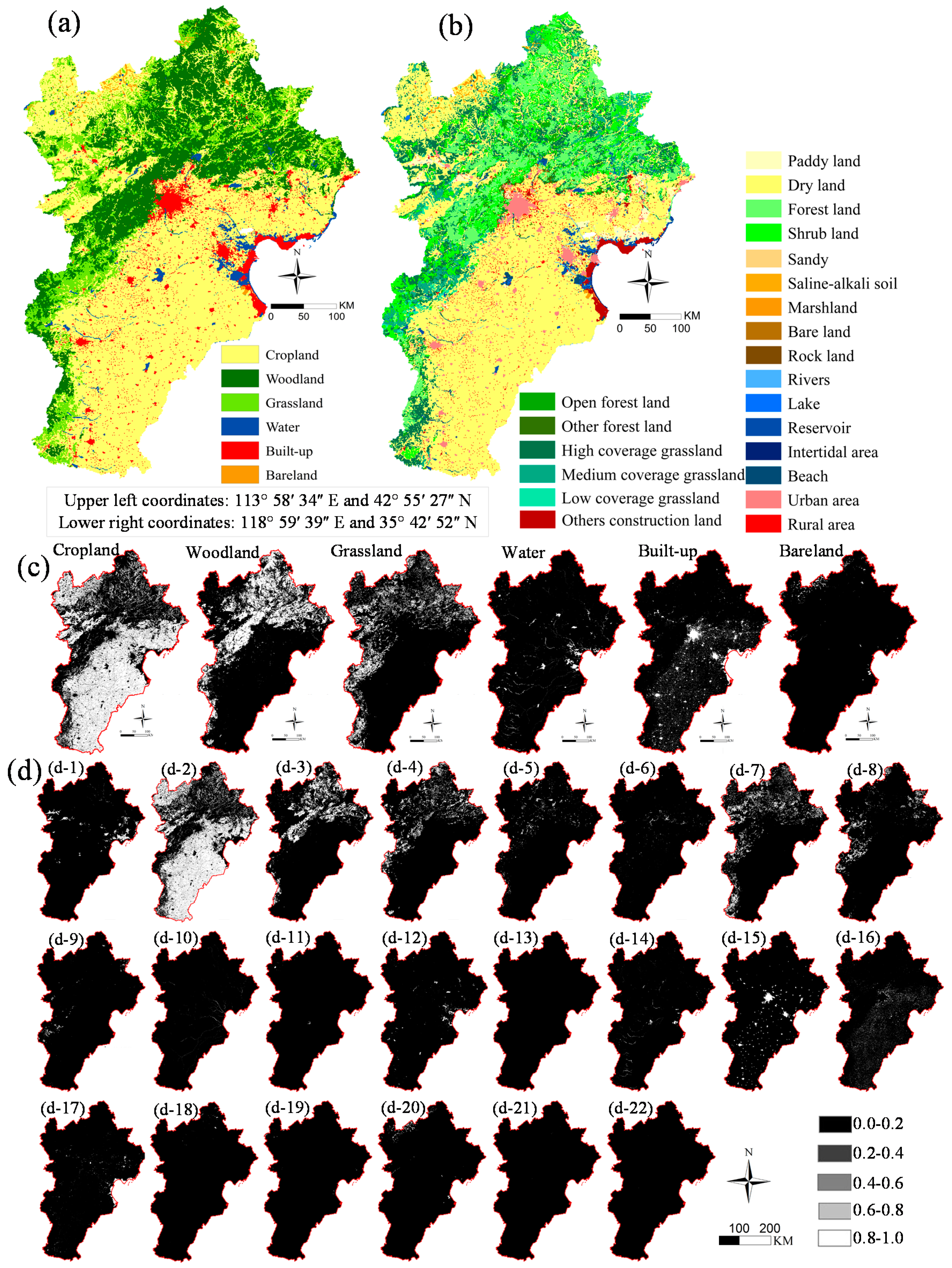
We distinguish two ways to obtain fraction images: soft classification from real remote sensing images and generation from existing LULC datasets such as upscaled data from high spatial-resolution classification data. For real remote sensing images, soft classification uses a classifier, such as a Bayesian or a support vector machine soft classifier, to directly generate fraction images with values ranging from 0 to 1 that indicate the proportion or possibility of pixels belonging to each class. Another way to extract fraction images is to aggregate existing classification data to simulate the output of soft classification, such as the Resources and Environmental Scientific Data Center of the Chinese Academy of Sciences [
34], National Land Cover Data 1992 [
35], and Global Land Cover datasets [
36]. Usually, a mean filter (such as 3 × 3 pixels) or a regular polygon are used to calculate the class proportions within the mean filter or the polygon from the existing classification data to produce fraction images [
7,
13,
17,
18,
33].
Reference data can be obtained in two ways: (1) validation points of ground truth for the SPM of real remote sensing images; and (2) reference maps for the SPM of synthetic fraction images degraded from existing classification data. Note that, for synthetic fraction images, each SPM map should have its corresponding reference map to ensure they have the same spatial resolution and size. The reference map is classified maps, which can be aggregated from existing classification datasets. More details for the generation of the reference maps can be discussed in
Section 3.1.
2.1.2. Setting Zoom Factors
The zoom factor Z is a critical parameter that divides each coarse pixel in the fraction images into Z × Z finer subpixels. With the zoom factor of Z, the number of subpixels for each class within mixed pixels can be calculated by multiplying the class proportion by Z2. Theoretically, it could be any integer value (>1) but an appropriate zoom factor should meet three requirements: (1) express the surface adequately; (2) retain the accuracy within an acceptable range; and (3) provide SPM output at the desired spatial resolution for practical applications, e.g., change detection requires maps with the same spatial resolution pertaining to different times. Therefore, selection of the optimal zoom factor could be considered the search for the optimal scale of SPM and several zoom factors should be tested and compared.
2.1.3. Selecting the SPM Algorithm
Different methods are suited to different situations because each has its own characteristics. Most SPM methods are based on spatial correlation, and therefore they are good at dealing with areal patterns. Some of these, such as pixel swapping [
13] and Hopfield neural networks [
9], involve iteration processes; thus, they require longer processing time. Others, such as geostatistics [
37], are based on pattern prediction, and are more suited to dealing with point features. These methods use training images to predict subpixel distributions, and therefore auxiliary high-spatial-resolution data are essential for the training sample. Selection of any SPM method should meet the requirements of the application according to the specific situation, e.g., different land surfaces or types of LULC classes. To explore the potential of different SPM methods, two or more representative SPM methods should be used.
2.2. Step 2: Assessment of the SPM Output
SPM output is usually assessed using a confusion matrix and its statistical metrics. The reference data for the accuracy assessment are considered the correct classification of the surface; thus, the agreement between the SPM output and the reference data is considered to reflect the effectiveness of the SPM. In SPM, the spatial pattern of LULC is also significant in determining the classification results and to their accuracies. Thus, the SPM output is assessed in terms of accuracy assessments and the values of the landscape pattern index [
38].
2.2.1. Accuracy Assessment
The accuracy of the SPM output is evaluated using a confusion matrix [
2]. This matrix presents the differences between the SPM output and the reference data, where the diagonal elements show correct classifications and the others represent commission and omission errors for each class [
2]. Four accuracy assessment indices (OA, KP, PA, and UA) are extracted from the confusion matrices to provide a quantitative assessment of the SPM results [
2]. Both OA and KP measure the degree of agreement between the classification results and the reference data [
2]. The difference between OA and KP is that KP excludes the possibility that a pixel might be classified correctly by randomness [
2]. PA measures the ratio of pixels within a certain class in the reference map that are classified correctly in the classification map. Similarly, UA measures the ratio of pixels classified as a specific class in the classification map with those that are actually in that class in the reference map. In the experimental design, the accuracy of the SPM results with different zoom factors, at different class levels, and using different SPM methods are assessed and compared. Note, similar to traditional accuracy assessments for classified maps of remote sensing imagery, all subpixels within both pure and mixed pixels of fraction images can be used in the accuracy assessment, because the experimental design aims to investigate the overall performance of SPM for practical applications and because the LSI and the APP are calculated in an area including both pure and mixed pixels.
2.2.2. Landscape Heterogeneity Analysis
The LSI represents the measurement of spatial patterns, which could be the measurement of area/edge, shape, core area, and aggregation. It can be calculated at both the landscape and the class level, reflecting the measurement of the spatial pattern of the classification data over an entire area or for each class, respectively. Of the various indices, the LSI is chosen as a measurement of surface complexity because it has a direct interpretation for landscape heterogeneity [
39]. It is defined as the total length of patch edges within a landscape, divided by the total area, and adjusted by a constant for a square standard. It is represented as
where
E is the edge length and
A is the patch area. The value of LSI begins at one and increases without limit as the landscape shape becomes increasingly irregular. Note that the calculation of LSI needs classified maps and each classified map can produce a LSI value by Equation (1).
2.2.3. Areal Pattern Proportion
The APP is an index with which to evaluate the areal spatial pattern, because most existing SPM methods are suited to areal features [
16,
18,
24,
25,
40]. The APP is equal to the area of features with areal pattern, divided by the total area:
where
Aarea is the area of the areal features,
Alinear is the area of features with linear pattern, and
Apoint is the area of features with point pattern [
33]. The sum of
Aarea,
Alinear and
Apoint is the total area.
Aarea,
Alinear and
Apoint are extracted by a feature pattern recognition method [
33]. First, all features are segmented by the seeded region-growing model from each fraction image. Second, the shape-density index is calculated for each extracted feature. Last, features are divided into the three types according to different values of shape-density index. More details can be found in [
33].
2.2.4. Combined Index
Both the LSI and the APP affect the performance of the SPM output. A CI of LSI and APP is developed next to assess the performance of the SPM results:
where
and
are control parameters that balance the contribution of LSI and APP. To control the range of parameters (−1 to 1) and of
(0 to 1), the LSI is normalized into the range of 0 to 1.
2.2.5. Representative Spatial Pattern Classes
To investigate the performance of SPM in dealing with features with different spatial patterns, some LULC classes are selected as representatives of areal, linear, and point features. In Geographical Information Sciences research, geographical features are usually generalized and classified into three types,
i.e., polygon, polyline, and point, and these three patterns have been considered in many applications [
33]. Areal features refer to high-resolution (H-resolution) cases where pixels are smaller than the features of interest, such as cropland and lakes, while point features refer to low-resolution (L-resolution) cases where pixels are larger than the features of interest [
8], e.g., buildings. Linear features differ from both areal and point features because pixels within this pattern are both shorter and wider than the features of interest and they typically retain connectivity [
33], e.g., roads.
2.3. Step 3: Analysis of SPM Performance
2.3.1. SPM Performance with Different Zoom Factors
Based on the accuracy assessment of all SPM output, the change of accuracy with different zoom factors is analyzed. The accuracy might decrease with increasing zoom factor [
6,
24,
40,
41], and therefore we are interested in establishing at which zoom factor the accuracy stabilizes.
2.3.2. SPM Performance of Different Classification Levels
Accuracies of SPM output at different classification levels are analyzed and compared. In a hierarchical classification system, different classification levels reflect the surface to differing degrees and they have different class amounts that also influence the SPM output.
2.3.3. SPM Performance of Different SPM Methods
The SPM output produced by different SPM methods is compared, and both similarities and differences are explored. The accuracy range and its change over the entire study area and for each class could also be discussed.
2.3.4. SPM Performance in Subareas with Different LSI Values
The spatial distribution of measurements calculated in subareas could be used to analyze SPM performance with different LSI values. The change of accuracy with LSI value can be illustrated using a scatterplot of measurements in subareas, where the LSI value is plotted as the x-axis and the accuracy assessment, such as OA and PA, is plotted as the y-axis. The accuracy assessment for different LSI ranges and the correlations between LSI and the accuracy assessment are calculated to explore the relationship between accuracy and LSI.
2.3.5. SPM Performance of Different Spatial Distribution Patterns
LULC classes with areal, linear, and point features are selected as representative features. Their accuracy assessments are compared to investigate the performance of SPM in dealing with different types of feature. Furthermore, the relationship between the APP values and accuracy assessments is discussed, as are the scatterplots of measurements in subareas for the APP values and accuracy assessments, and the correlation values between the APP and accuracy assessment.
2.3.6. Analysis of SPM Performance with CI Value
To analyze the relationship of SPM performance with both LSI and APP, the LSI and APP values are used as variables in a regression of accuracy assessments to obtain an estimation equation. Thus, when the LSI and APP values of a subarea are known, the equation could be used to estimate the performance of SPM and consequently, to determine whether the use of SPM is appropriate. Note, when exploring the relationship of the SPM results with the LSI, APP, and CI values, the LSI, APP, and CI indices and the accuracy of SPM results are calculated in county subareas.
4. Discussion
4.1. SPM Performance with Change of Zoom Factor
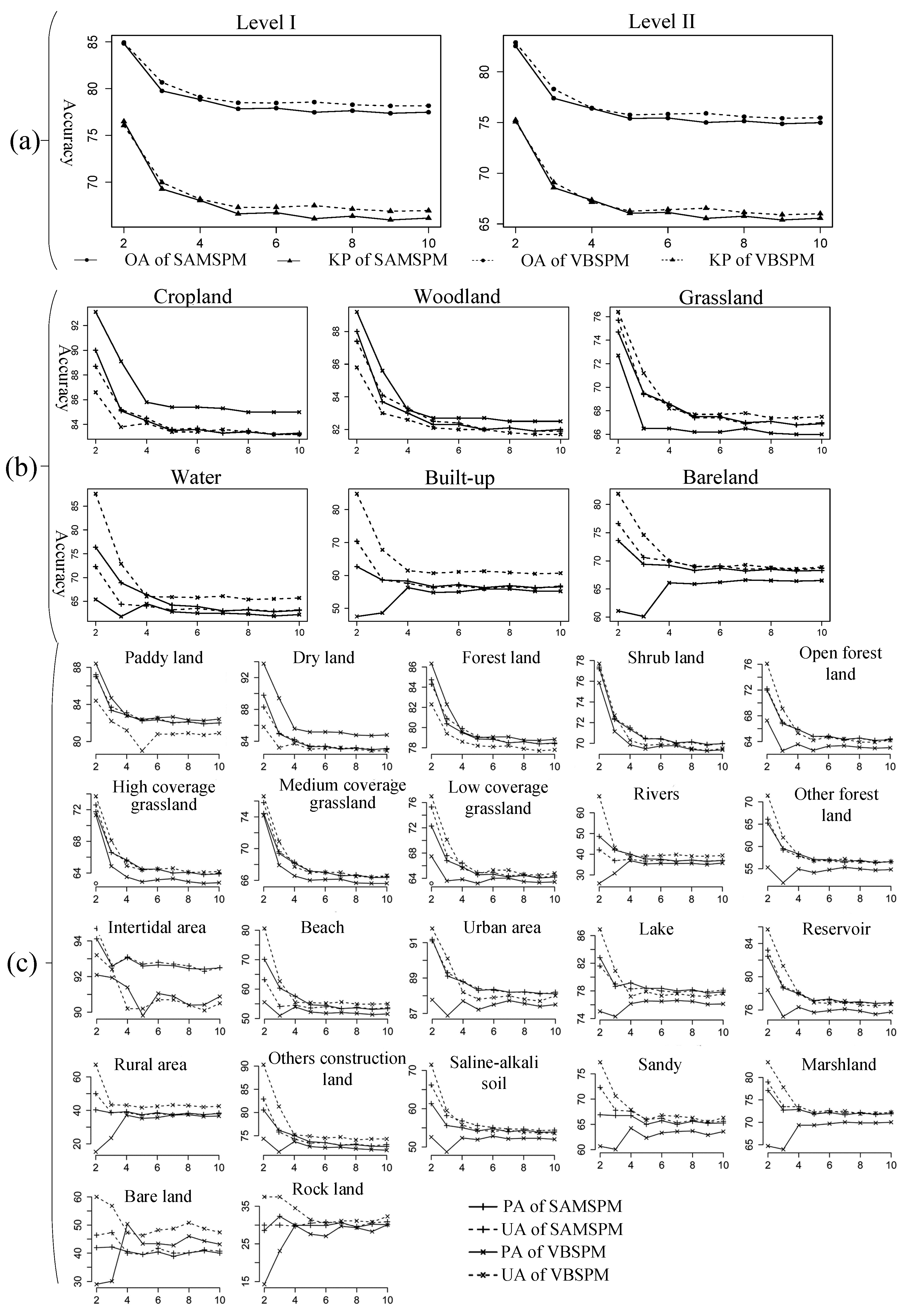
This study shows that OA and KP generally decrease as the spatial resolution of the SPM results becomes finer with the increase of the zoom factor. The reason for this can be attributed to the increase in the number of subpixels within a coarse pixel as the zoom factor increases; thus, greater uncertainty is generated regarding class allocation of the subpixels [
25,
40]. The reason for the stability of the accuracy assessment when the zoom factor is above five is that the proportion of mixed pixels within the 1-km fraction images becomes stable at this zoom factor. This is because the criterion defining mixed or pure pixels depends upon the zoom factor. As an illustration, it can be seen that the spatial resolution changes from 500 to 200 m when the zoom factor increases from 2 to 5, whereas it changes from 200 to 100 m when the zoom factor increases from 5 to 10.
4.2. SPM Performance at the Two Classification Levels
Comparing the accuracy assessments of the SPM results at the two classification levels reveals that classes with areal patterns at Level II, subdivided from Level I, have similar PA and UA values as those at Level I because of the similarities in their distribution patterns. For example, the PA of dry land (83%–94%), subdivided from cropland, is close to cropland (83%–93%). Classes with linear or point patterns, however, are different from classes with areal patterns. For example, the classes of intertidal areas and rivers at Level II, subdivided from water, have different accuracies. Intertidal areas have high accuracy (>90%) and rivers have low accuracy (<68%), whereas the accuracy of water is 62%–88%. Another example is built-up areas (58%–64%) at Level I, which has the subclass of rural areas (<40%) with a point pattern.
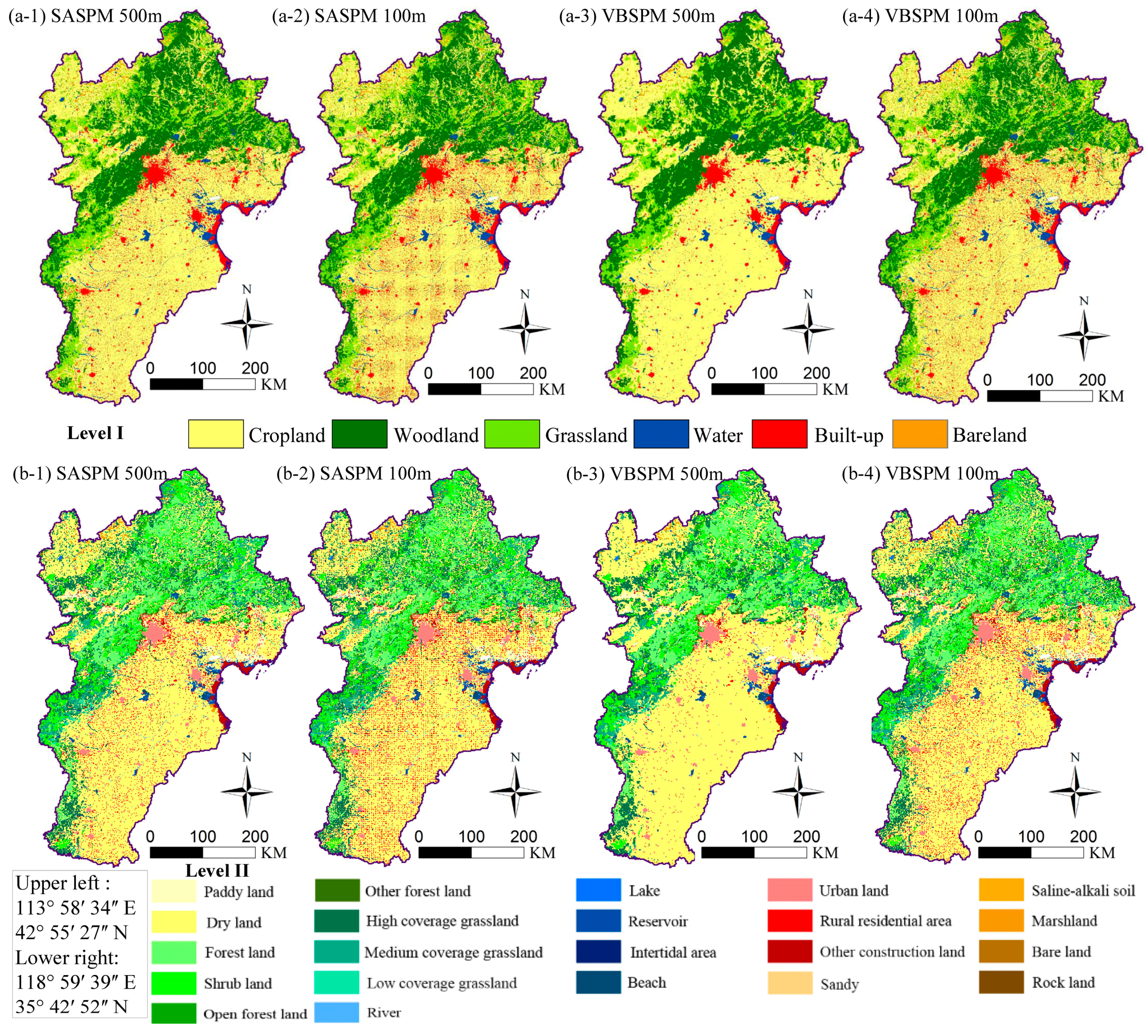
4.3. Performances of SAMSPM and VBSPM
Both SAMSPM and VBSPM perform well in the experiments and produce equivalent accuracies in different areas, but some differences remain in the detail (
Figure 10). VBSPM produces slightly better results with greater OA (range: 0.3%–1.1%) than SAMSPM. VBSPM, however, generates results for built-up areas at Level I and rivers, rural areas, and rock land at Level II that are slightly less accurate (<1%) than SAMSPM with a low zoom factor (<4). This is because these classes do not represent H-resolution cases, for which VBSPM is most applicable [
27]. The different performances between SAMSPM and VBSPM in these classes, however, have only minor influence on the OA.
4.4. SPM Performance in Subareas with Different Landscape Heterogeneity
A scatterplot is used to investigate the relationship between accuracy and LSI values. It shows that the OA and PA both decline with increasing surface complexity, which is measured by LSI. For the entire image, the less complex the surface, the better SPM performs. The complexity of the surface for the entire area and for each class can be measured separately by LSI at both the landscape (all classes) and the class level. For example, the experiment shows that subareas with LSI values in the range 1–4 have OA values of about 85%, subareas with LSI values in the range 4–10 have OA values of about 77%, and subareas with LSI values >10 have average OA values of about 70%. However, at the class level, PA is not always consistent with the LSI value. Usually, classes with H-resolution features (e.g., cropland and woodland) have relatively high PA values. Some classes with point features (e.g., water and built-up areas) have relatively low LSI and low PA values, because SPM does not perform well when dealing with point features. Areal features with lower LSI values have higher PA values than point features with low LSI values.
4.5. SPM Performance of Point, Linear, and Areal Pattern Classes
Among the three spatial patterns, classes with areal pattern have the highest accuracy. One explanation for this is that areal features have strong spatial correlation between pixels and subpixels; thus, those SPM methods based on the assumption of spatial dependence are well able to deal with such correlation, especially VBSPM. A second explanation is that the object size of areal features is generally much larger than the pixel size; thus, it contains a relatively large proportion of pure pixels that can lead to relatively high accuracy in the downscaled classification. Because the SPM methods used in this study are based on the assumption of spatial correlation, land use classes with linear patterns, such as rivers, often do not remain contiguous in the SPM results; thus, their accuracy is not high, especially for linear features with small widths. However, classes with point patterns have the lowest accuracy assessment among the three spatial patterns. This is because greater uncertainty in predicting the spatial locations of point features is generated because of the fewer constraints or lack of complementary information. Atkinson [
8] stated that the goal of SPM for point features is to predict patterns rather than to generate an accurate prediction on a subpixel-by-subpixel basis. Thus, some SPM algorithms based on pattern prediction may be more suited to mapping land use classes with point patterns [
33].
4.6. Analysis of SPM Performance with CI Value
The CI is a linear combination of the LSI and APP, which are the two indices related to SPM performance. The values of the regression parameters reveal that the contributions of the two indices may vary for different areas and different classes. For all classes, CI is similar to LSI, which indicates that the less complex the area, the less impact APP has and the better SPM may perform. At the class level, CI has different combinations of the LSI and APP. The SPM performance is better for smaller values of LSI and larger values of APP. Generally, CI could be used as an indicator to predict the performance of SPM prior to its use in practical applications.
4.7. Uncertainty of SPM Caused by Fraction Images of Soft Classification
The experiment uses the error free fraction images to avoid the impact of the uncertainty in soft classification on the SPM results. Actually, uncertainty or errors in soft classification are inevitable when classifying real remote sensing images [
27]. As a result, uncertainty or errors from the soft classification of real remote sensing images would be propagated into SPM and the accuracy of SPM would be decreased. Ge [
4] proposed a solution using the multiple-point simulation to reduce the uncertainty or errors in soft classification and it can be used in future SPM experiments on real remote sensing images.
4.8. Potential of SPM as an Alternative Method for Generating LULC Maps
Using the 1-km synthetic fraction images, the SPM methods based on the assumption of spatial dependence are able to produce land use maps at subpixel scales, with OA values of 77%–85% and 75%–83% for the six classes at Level I and 22 classes at Level II, respectively, over the large area of Jingjinji region in China. These accuracies decline with the increase of S, and stabilize at an OA of approximately 78% at Level I and 75% at Level II, when the zoom factor reaches five. The two SPM methods produce the highest accuracy for areal pattern classes (e.g., cropland, woodland, and grassland), medium accuracy for linear pattern classes (e.g., water), and the lowest accuracy for point pattern classes (e.g., bare land and built-up areas). In the subareas (i.e., counties), less complex areas exhibit higher accuracy; i.e., subareas with high LSI values have lower accuracy, and subareas with LSI values of <18 generate SPM results with OAs of >80%.
In summary, according to the SPM output, SPM has the potential to generate alternative LULC maps for regions where high-spatial-resolution maps are unavailable, especially in less complex areas with a large proportion of areal features. Thus, when using SPM to obtain finer-resolution LULC maps from real coarse remote sensing images or existing fraction images in future applications, the experimental design can be used. A primary assessment of the LSI and APP can be done to provide an indication of the most suitable method and to determine the appropriate zoom factor and classification system to use.
5. Conclusions
The objective of this study was to investigate the feasibility of using subpixel mapping (SPM) to obtain land use/land cover (LULC) data in the absence of high-spatial-resolution LULC maps. An experimental design was proposed to evaluate its feasibility for providing alternative LULC maps based on accuracy assessments and landscape measurements. In accordance with the experimental design, a case study was implemented in the Jingjinji region of China using 1-km land use fraction imagery as input data, the landscape shape index (LSI) as the measurement of surface complexity, and areal pattern proportion as the measurement of the spatial distribution pattern of geographical features. The results and analysis showed that overall accuracy (OA) was approximately 80% and that the accuracy declined with increasing zoom factor before stabilizing at a zoom factor of five. The accuracy of SPM was apparently associated with both the complexity and spatial pattern of the geographical features. Higher accuracy was obtained in less complex areas and when handling areal features, compared with handling linear and point features. Subareas with LSI values <4 showed OA values of approximately 85%, subareas with LSI values of 4–10 showed OA values of approximately 77%, and subareas with LSI values >10 had OA values of approximately 70%.
This experiment used an existing proportional land use dataset. In the future, soft classification results derived from remote sensing images should also be practicable. Moreover, other newly developed SPM methods, such as pattern-prediction-based SPM, might be worth consideration. Therefore, it would be interesting in the future to repeat this experiment using other SPM algorithms and actual remotely sensed images.


