Article

Estimating Tree Frontal Area in Urban Areas Using Terrestrial LiDAR Data

1
Center for Urban and Environmental Change, Indiana State University, Terre Haute, IN 47809, USA
2
Department of Earth and Environmental Systems, Indiana State University, Terre Haute, IN 47809, USA
3
Department of Mathematics and Computer Science, Indiana State University, Terre Haute, IN 47809, USA
*
Author to whom correspondence should be addressed.
Remote Sens. 2016, 8(5), 401; https://doi.org/10.3390/rs8050401
Submission received: 9 March 2016 / Revised: 16 April 2016 / Accepted: 4 May 2016 / Published: 11 May 2016

Abstract

:
Surface roughness parameters, such as roughness length and displacement height, impact the estimation of surface moisture, and the frontal areas of buildings and trees are two components that contribute to surface roughness in urban areas. Research on tree frontal area has not been conducted in urban areas before, and we hope to fill that gap in the literature with this study by using Terrestrial Light Detection and Ranging (LiDAR) data to estimate tree frontal areas in Warren Township, Indianapolis, IN, USA. We first estimated the frontal areas of individual trees based on their morphology, then calibrated a regression model to estimate the tree frontal area in 30 m pixels using parameters derived from LiDAR data and tree inventory data. The parameters included tree crown base area, height, width, conditions, defects, maintenances, genera, and land use. The validation shows that R2 yielded values ranging from 0.84 to 0.88, and RMSEs varied with tree category. The tree categories were identified based on the height and broadness of the canopy, which indicated the degree of resistance to air flow. This type of model can be used to empirically determine local roughness values at the tree-level for any city with a complete tree inventory. With the strong correlation between trees’ frontal area and crown base area, this model may also be used to determine local roughness value at 30 m resolution with NLCD (National Land Cover Database) tree canopy cover data as a component. A proper tree categorization according to the vertical air resistance, e.g., height and canopy density, was effective to reduce the RMSE in tree frontal area estimation. Geometric parameters, such as height, crown base height, and crown base area extracted from Airborne LiDAR, which demand less storage and computation capacity, may also be sufficient for tree frontal area estimation in the areas where Terrestrial LiDAR is not available.

Graphical Abstract

1. Introduction

A better knowledge of the controls of the urban heat island effect is important for estimating the impact of global climate change on urban areas. The limited number of weather stations in urban areas is often not sufficient to delineate the spatial distribution of air temperature, and the estimation of Land Surface Temperature (LST) from remotely sensed data has attracted more and more attention [1]. Therefore, factors that link air temperature and LST are important in urban heat island studies [2,3]. One of them is surface moisture. The Two Source Energy Balance (TSEB) Model has been used in forest and agricultural areas to estimate evapotranspiration over soil and vegetation surfaces. When applying the TSEB to urban areas to estimate evaporation over impervious surfaces, a great challenge is that the original model did not consider urban morphology [4,5,6]. Urban areas are not flat plains; they include open spaces, roofs, and canyons, which represent volumes [7]. The two major components to surface roughness are buildings and urban trees in urban areas.
Surface roughness refers to aerodynamic properties related to the height of objects. It impacts the wind speed and consequently surface moisture. Usually, surface roughness can be described by roughness length and displacement height. Conventional ways to measure surface roughness have disadvantages and high uncertainty. The disadvantage of micrometeorological wind profile measurement [8] is that it is expensive, site specific, and limited to the source area. Therefore, it cannot be applied at a broader scale. The wind tunnel method [9] relies on lab simulations on simplified geometrics, and thus it sacrifices from actual complex geometries and needs field validation [10]. The aerodynamic properties of urban areas have also been tested by morphometric methods based on analysis of surface forms, and found that the morphometric methods yielded reasonable estimations of displacement height and roughness length [9]. Three approaches for estimating aerodynamic properties (displacement height and roughness length) in urban areas were categorized as: (1) height based approach; (2) height and plan areal fraction approach; and (3) height and frontal area index approach [11,12,13]. However, the statistical agreement between measured roughness data and the morphometric estimates of roughness parameters was poor at 11 sites in seven North American cities. Partly, that was due to uncertainties in observation and analysis of winds over inhomogeneous surfaces and the necessary simplification of geometric descriptions. Therefore, among the three approaches, the best one was the height and frontal area index approach [9]. Heights of objects can be easily estimated from DEM and DSM, but frontal areas are a bit complicated. Burian and his colleagues conducted morphological analyses to several major cities in the U.S. [14,15,16]. However, these studies considered only buildings; tree frontal area estimation has not yet been done in urban areas.
Tree frontal area is the vertical projected area that faces wind or water flow direction [17]. In urban areas, wind direction usually goes along the urban canyons [15]; Terrestrial LiDAR data collected by vehicles along streets provide great potential for capturing the complex vertical structure. Although [17] estimated leafless tree frontal areas using Terrestrial LiDAR data in a riparian forest, it only scanned three poplar trees individually. To estimate tree frontal area in a larger geographical scale, classification of vegetation is the first important step. The concept of object surfaces in point cloud was used to grow planar and smaller surfaces, which differentiate vegetated and non-vegetated objects [18,19,20,21,22]. Rutzinger et al. [23] used this segmentation method on Terrestrial LiDAR to separate trees from non-vegetated surfaces, applied Alpha shapes to reduce the point density and get the outer shape of trees, and then 3D tree models that allows detailed reconstruction of branching structure and leaf texture were created. One of the important steps that were not emphasized in [23] was the individual tree segmentation. The experiments of individual tree segmentation were conducted on airborne LiDAR with the watershed algorithms [24,25] and in forests on a small footprint with similar tree species [26,27]. Li et al. [26] proposed a top–down method for separating the coniferous trees based on their cone shape. Lu et al. [27] used a bottom–up method to separate the deciduous trees. The study area of [23] was on a slope, and the airborne LiDAR data was collected not from the top but the side of the trees. Moreover, the algorithm of [27] detected the trunk and branches first and then added the rest of the points, which is applicable for Terrestrial LiDAR.
Although methods have been developed to extract geometric information from Terrestrial LiDAR, they have not been used to extract roughness related parameters for urban-micrometeorology studies. In addition, the combination of Terrestrial LiDAR estimates and raster data has great potential to fill the gaps in currently available surface moisture models. Therefore this study proposed a method of using Terrestrial LiDAR to estimate the frontal area of individual urban trees, and combined the information from tree inventory, Landsat images, and tree canopy cover data to calculate the tree frontal in 30 m pixels.

2. Data and Methods

2.1. Study Area

The study area, Marion County (Figure 1), is the county seat of Indianapolis, in the State of Indiana. Marion County is part of the Indianapolis-Carmel-Anderson Metropolitan Statistical Area. Located on a flat plain makes it possible for the city to expand in all directions. Indianapolis was the 14th largest city in the United States by population in 2014. The area lies between latitudes 39°55′37.75″N to 39°37′54.28″N and longitudes −86°19′33.65″W to −85°56′10.11″W. According to the 2010 Census, the total area of Marion County is 1044 km2 of which 98.34% is land and 1.66% is water.

2.2. Dataset

Terrestrial LiDAR data were acquired from Indianapolis Mapping and Geographic Infrastructure System (IMAGIS). The data was collected in 2012 and 2013, covering all streets in Marion County. The point density is 1000–2000 points per square meter. The Terrestrial LiDAR data was generated from Lynx MG1 Model Mapper mounted on roof rack, about 3 m above ground. The two sensors produced 1,000,000 points per second. The maximum range is 250 m at 10% reflectivity, the range precision is 5 mm, and absolute accuracy is ±20 cm. The two sensors shot lasers to two sides of the road and collected 3D point cloud of the laser reflectance. Mobile LiDAR saves both cost and time because it can gather all required data point measurements in one setting, eliminating the need for additional mobilization costs, and it gives us the ability to collect up to 1,000,000 points per second, compared to one point every few seconds with conventional survey technologies. The Terrestrial LiDAR data will be used to calculate tree frontal area of individual trees. Tree inventory data and township shapefile were acquired from the Department of Public Works, City of Indianapolis. It includes the location of the trees, tree genera, tree species, DBH, conditions, maintenances, defects and so on. A Landsat 8 image was acquired on 6 September, 2013 from Earth Explorer, and tree canopy cover data from the 2011 National Land Cover Database (NLCD) was used for tree frontal area estimation. Normalized Difference Vegetation Index (NDVI) will be calculated from the Landsat image. NDVI, tree canopy cover, and the highly correlated factors from tree inventory data will be used to estimate the tree frontal area in each 30 m pixel.

2.3. Methodology

To estimate the frontal areas of urban trees, two steps were taken. First, the frontal areas of individual trees were estimated from Terrestrial LiDAR data. Second, regressions were formed for each tree category to estimate the frontal area per 30 m pixel, and thus the tree frontal area for the whole study area was estimated. Figure 2 shows the workflow, and the following sections describe the method in detail.

2.3.1. Estimation of Individual Tree Frontal Area

After removing ground, LiDAR point cloud was segmented into homogeneous planar regions [18,23]. Then large segments such as roofs and walls were removed, and the remaining segments were relabeled by grouping nearby points to connect components. The connect components of trees were detected by the roughness measured by the standard deviation of elevation, and the point density ratio [23]. The point density ratio is calculated between the total number of points and the number of points below a certain height, because tree trunks usually have less laser echoes compared to tree crowns. The height used in the ratio calculation was 0.5 m. The thresholds were set for selecting high standard deviation and low point density ratio.
The algorithm for individual tree segmentation was based on a bottom–up method developed by [27]. In each connect component, the points bounced back by trunk and braches were selected with a threshold in intensity. From the bottom up, the horizontal distance between the points on the trunk and branches were calculated, and the points within a certain distance threshold were segmented into one tree. After building the trunk and branches, the rest of the points were allocated to the existing trees according to the 3D distance from the nearest trunk or branch. To estimate the frontal area for individual tree, the point cloud of each individual tree was projected onto a vertical plain by assigning the mean x value or mean y value to all points. Then grids were formed on the 2D projection area. Points were filled on grids, and the number of grid with points was counted. The grid size was decided according to the point density. The frontal area results were compared with the existing literature [17], and the optimal grid size was decided.

2.3.2. Green Vegetation Abundance Contributed by Trees

NDVI can measure the abundance of green vegetation. Tree canopy cover is the proportion of an area covered by the vertical projection of tree crowns [28]. In urban areas, not all green vegetation abundance was contributed by trees; another major contributor is lawn. The multiplication of NDVI and tree canopy cover resulted in the green vegetation abundance contributed by trees. NDVI was calculated by using surface reflectance of band 4 and band 5 from Landsat 8 images. The raster pixels were then converted to points by using the coordinates of mean x and mean y as the location of the tree, with frontal area, tree crown base area, height, length, and width in the attribute table.

2.3.3. Tree Categories

In the tree inventory dataset, 30 genera of trees were found in the study area (Table 1). For the purpose of estimating the frontal area, the characteristics of vertical shapes described by the height and canopy size were used to categorize the trees into bigger categories.
Understory (U), Intermediate (I), and Dominant (D) were used to describe the height of a tree, while Broad canopy (B) and Sparse canopy (S) were used to describe the density of the canopy. These characteristics were used because it directly related to the resistance to air flow. Coniferous trees were a large category in the study area; they fell in the category of Dominant broad canopy. However, since the vertical shape of coniferous trees was distinct from deciduous trees, and the canopy density was usually higher, we designed a special group for conifer trees (Group 7). The detailed tree category table can be found in the Appendix A.

2.3.4. Tree Frontal Area Estimation in 30 m Pixels

The variables of individual tree were added together in each 30 m pixel. The numeric variables, such as DBH and height, became the sum in each 30 m pixel; the dummy variables, such as trees in poor condition and trees in single-family residential land, became number of trees with under those conditions in 30 m pixels. Pearson Correlation between the variables and tree frontal areas in each 30 m pixel were calculated, and the variables with higher correlation (>0.5) were selected to form stepwise multivariate linear regression models.
The northern half of Warren Township was used as the calibration site, and the southern half as the validation site (Figure 3). NDVI and tree canopy cover were multiplied to obtain green vegetation abundance contributed by trees. The 30 m resolution raster was then converted to points. Each point represented the center of a pixel. Tree inventory with LiDAR extracted crown base area, height, width, and depth of each tree, and the frontal area were associated with values of NDVI and tree canopy cover. The sum of the values of tree frontal areas was calculated for trees within each pixel. There were 250 training samples, and 319 validation samples. Pearson correlation was conducted between frontal area and the factors to estimate frontal areas, such as NDVI, tree canopy cover, geometric parameters of trees, and the records in tree inventory. The following paragraphs in this section describe more details of the parameters from both Terrestrial LiDAR and tree inventory data, and their relationships with tree frontal area.
The variables relevant to tree frontal area were selected from the tree inventory data, including DBH, tree condition, tree damages, land use types, maintenance, and defects. DBH ranged from 1 inch to more than 42 inches. Although it varied from species to species; larger DBH often indicated larger frontal areas. Tree condition was described as dead/dying, poor, fair, and good. The trees in a dead/dying condition may not necessarily possessed less frontal area, however, the amount of new branches and leaves may be reduced on the dying trees. As a result, the frontal area may be smaller compared to trees in the same species and of the same age in healthy conditions. Similarly, good condition trees may grow more leaves and new branches, which may result in bigger frontal areas. The four tree condition categories were described in dummy variables in the regression model. Primary maintenance to trees included large tree cleaning, small tree cleaning, young tree training and planting new trees. These actions were grouped into two categories based on their function to potentially increase or decrease the fontal area, and dummy variables were used for the two categories. Since removal and stump removal would result in no tree present at that location, these trees were taken out of the analysis. Secondary maintenance included raise, reduce, thin, restoration, utility, and the default was none. As primary maintenance, dummy variables were used, and none was the control group.
There is a list of 32 types of tree damages, including adventitious, cavity, completely topped, construction damage, and infested by Emerald Ash and Borer (EAB). The default was no damage, and up to two major damages were recorded. Dummy variables were used to describe this information and no damage was the control group. The sizes of defects were categorized as N/A, less than 4 inches, 4–20 inches, and greater than 20 inches in the tree inventory. The categorical variables were expressed by dummy variables in the regression model.
Fahey et al. [29] found that responses of tree species to drought varied with land use, such as built-up, transportation, park, and semi-natural forest. Their test was conducted on four species: Acer saccharum, Gymnocladus dioicus, Liriodendron tulipifera, and Pinus strobus in suburban Lisle, Illinois, USA. Yearly growth for each tree was calculated by converting ring width to basal area increment (BAI) by back calculating basal area based on current diameter and annual ring widths. Their result showed that for all species, the highest yearly growth was found in parks, followed by built areas, transportation sites, and forests. The most important finding was that urban tree growth and resistance to drought varied as an interaction between species and land uses. In the tree inventory data, there were description of land use and site. Land use included single-family residential, multi-family residential, small commercial, industrial/large commercial, and park/vacant. Site types included front yard, planting strip, cutout/pit, median, other maintained locations, other unmaintained areas, side yard, backyard, row, and wooded edge. These variables were categorized as dummy variables in the regression model.
In addition to tree frontal area, other morphological parameters derived from Terrestrial LiDAR included tree height, tree width, and tree crown area. The estimations of tree heights and crown base area, were inspired by the voxel-based method proposed by [30].

3. Results

3.1. Frontal Area Estimation for Individual Trees

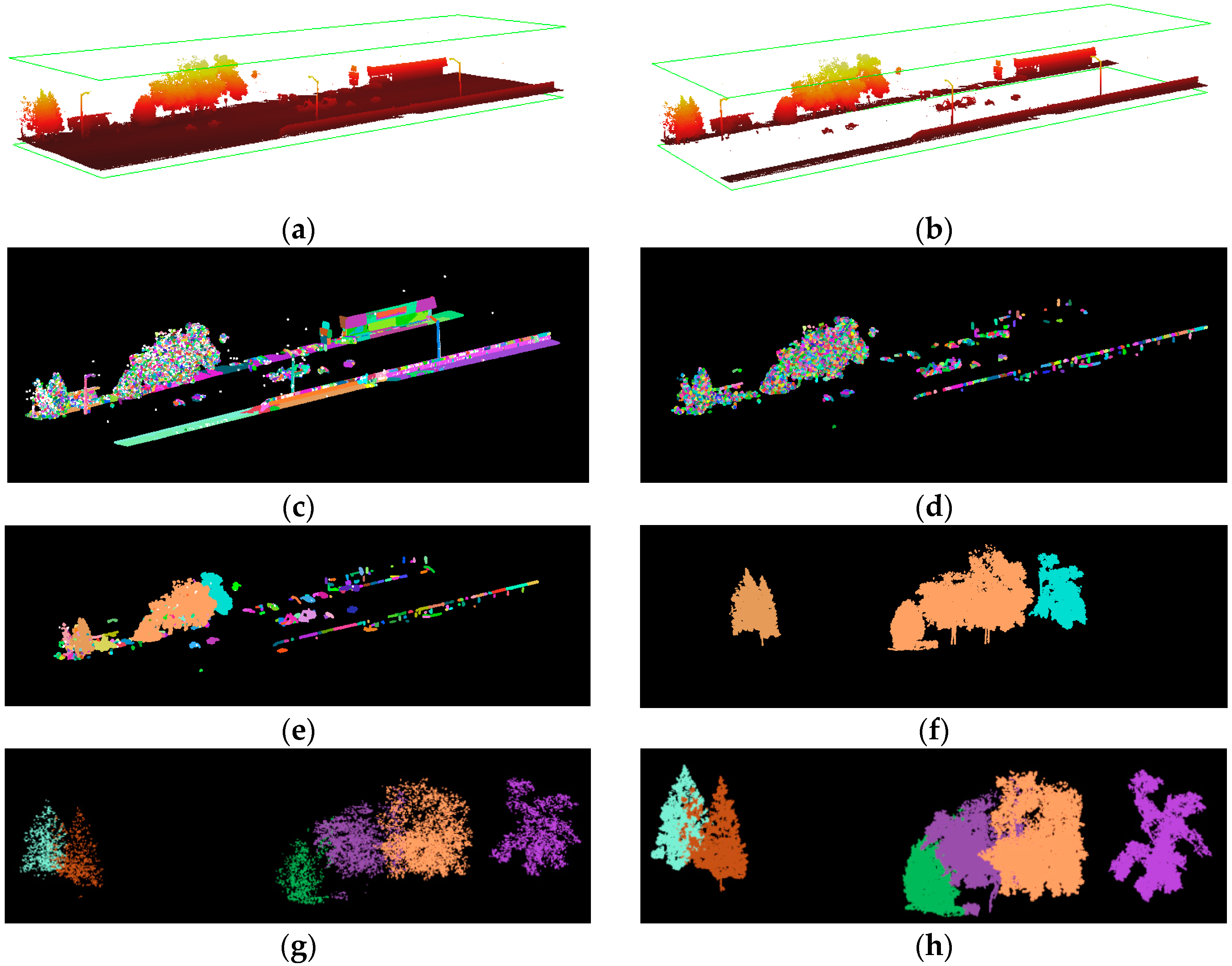
Figure 4a–h shows the process of individual tree segmentation on one Terrestrial LiDAR tile. The major steps included ground removal, surface growing, planar removal, connect components, tree detection, trunk and branch building for individual tree segmentation, and allocating the rest of the points. As shown in Figure 3, the proposed method successfully segmented both deciduous trees and coniferous trees. More specifically, Colorado Blue Spruce and Siberian Elm were the species recorded on the tree inventory data for the leftmost and rightmost ones. This method was suitable for urban areas with diverse tree types. It is worthy to note that the tree inventory only recorded trees on public lands; not every tree in the city was listed.
Five hundred Terrestrial LiDAR data tiles, around 1 TB data, were processed in this study. A total of 12,697 trees were detected: 433 trees were found matching with the 2013 tree inventory, and 711 trees with the 2014 tree inventory. The 2013 tree inventory covered the northern half of Warren Township, while the 2014 inventory covered the southern half of the Township. The number of matched trees was relatively small, because the tree inventory surveyed only trees on the land owned by the City of Indianapolis, but not those on private lands.
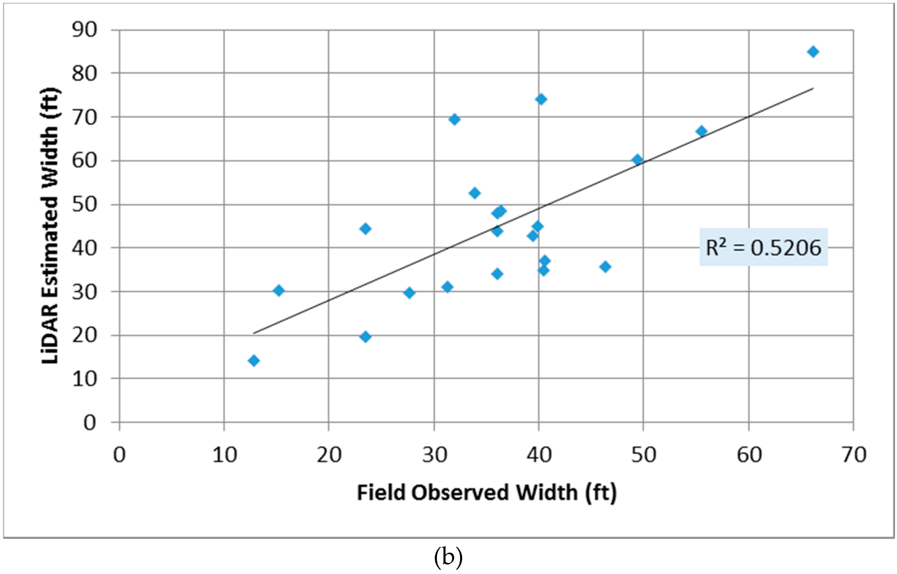
As described in the methodology section, in the individual tree frontal area estimation, a bounding box was formed for each individual tree. The lengths of z axis (height), x axis (along E-W direction), and y axis (along N-S direction) were included in the output. Since it was hard to visualize tree frontal area, we decided to use a proxy to validate our results. Width, height, and crown base area are proxies that related to frontal area. The correlation between the three proxies and frontal area are all greater than 0.9. However, width was the easiest to be measured in the field, and that is why we chose width, which was the side length of a tree along N-S direction for the purpose of validation. Three transects were selected, and the length of y axis of the bounding box of each tree was measured by tape. GPS locations were recorded, photos were taken, and the results were compared with the LiDAR estimates. Figure 5a shows the tree transects. The first transect was located 0.2 mile from New Life Community Church (6407 E 14th St.) to 6401 E 16th St., the second transect 0.4 mile from New Life Community Church (6345 Massachusetts Ave.) to the Marathon Gas Station (3399 N Arlington Ave.), and the third transect 0.3 mile from Marathon Gas Station (3399 N Arlington Ave.) to 6601 E 34th St. The first transect was in a residential area, while the second and third transects were along major roads. The three transects were chosen because they were on public lands, many trees matched the tree inventory data, and tree species and growing stages were diverse. Twenty-one trees were selected for the validation. The R2 was 0.52, and the RMSE was 15 feet (Figure 5b). This indicates that the individual tree segmentation, bounding box, and the choice of the size of the grid is reasonable in this case study.

3.2. Estimating Frontal Area for per 30 m Pixel

The correlation between each factor and the tree frontal area was calculated, and the factors that highly correlated with tree frontal area were selected for the stepwise linear regression model (Table 2).
Stepwise multivariate linear regression model (Model 1) was built between frontal area and the independent variables in Table 2. The R2 of the model yielded 0.99, and the standard error of the estimation was 77.35. It should be mentioned that not every city has complete tree inventory data, and not every tree inventory collects same types of data, and some variables can also be extracted from airborne LiDAR data. To make model more applicable to other areas, another multivariate regression model (Model 2) was built with only geometric variables, including DBH, crown base area, height, and width. The R2 of the model yielded 0.99, and the standard error of 77.48.
Since the crown base area discovered the highest correlation with the frontal area (0.99), the association between frontal area and crown base area was further explored. A linear regression model was built between frontal area and crown base area (Model 3). The R2 of the model yielded 0.98, and the standard error of the estimates was 103.89. The high R2 indicates the strong relationship between tree frontal area and tree crown base area. Therefore, for the areas that only have NLCD tree canopy area data available, this model can be used to estimate tree frontal area based on tree canopy cover data.

3.3. Model Validation

All three models were validated in the southern half of Warren Township, and the R2 and RMSE are shown in Figure 6. Thirty-nine additional tree types and 25 corresponding tree genera were found in the validation site but not in the calibration site. These trees were also categorized according to the same criteria as shown in Table 1. Adding the additional tree types in validation was to test if the models were robust for trees that were not found in the calibration models.
Model 1 is the multivariate regression model with all the independent variables with a correlation greater than 0.5; Model 2 is the multivariate regression model with only the geometric independent variables extracted from Terrestrial LiDAR; Model 3 is the regression model with only the crown base area, which has the highest correlation with frontal area (0.991).
Figure 6a shows that the overall R2 for Models 1 and 2 were similar, 0.87 and 0.88, respectively. The Model 3 yielded a relatively lower R2, 0.84. Similarly, while RMSE for Models 1 and 2 emulated each other, and RMSE of Model 3 was higher. This finding indicates that geometric variables were key to frontal area estimation, and adding more variables from tree inventory data may not significantly increase the robustness of modeling.
Further, R2 varied with tree category. Categories 1–6 had very high R2, greater than 0.94. Category 7 (conifer trees) detected a lower R2, 0.89 for both Models 1 and 2 and 0.74 for Model 3. This lower R2 can be attributable to the diversity of conifer trees. Eleven species were included in training samples, i.e., Arborvitae spp., Black Pine, Burkii Eastern Redcedar, Colorado Blue Spruce, Douglas Fir, Juniper, Northern White Cedar, Norway Spruce, Red Pine, Scotch Pine, and white pine. The relationship between tree frontal area and the independent variables may vary among different species in the big category of conifer trees. The RMSE of Model 3 is also much higher than other categories. Models 1 and 2 are better for this bigger group. If crown base area is the only variable available, finer sub-categories need to be divided for conifer trees.
According to Figure 6b, the individual categories yielded much smaller RMSE compared to blending 7 categories together. This indicates that the method of categorizing trees according to their height and canopy density is effective in tree frontal area estimation. Categories 1 (Understory and Sparse Canopy) and 4 (Intermediate and Broad Canopy) generated relatively high RMSE, both of greater than 200 ft2. Categories 2 (Understory and Broad Canopy) and 3 (Intermediate and Sparse Canopy) produced a lower RMSE, around 70 ft2 for the first two models. For Understory and Broad Canopy and Intermediate and Sparse Canopy trees, the addition of more geometric variables was helpful to increase the accuracy of the frontal area estimation. Category 5 (Dominant and Sparse Canopy) was a small group, including only Birch and Kentucky Coffeetree, whereas Category 6 (Dominant and Broad Canopy) the biggest group. For Category 6, Models 1 and 3 yielded the same RMSE (103.48 ft2), but Model 2 much lower RMSE, 83.75 ft2. Therefore, for Dominant and Broad canopy trees, geometric variables were key to frontal area estimation.
The optimal models for different tree categories were suggested. Model 3 generated high RMSE values for all tree categories, especially for Categories 2, 3, and 7. Therefore, for Categories 2, 3, 7, Models 1 and 2 were better choices. The accuracy of Models 1 and 2 did not show significant difference for all categories, but Model 2 did yield smaller RMSE than Model 1 for Categories 2 and 6. Therefore, for these two categories, variables from tree inventory data were not useful for frontal area estimation. Categories 1, 4, 7 yielded relatively large RMSE values compared to other categories; thus, finer categories and/or better models need to be developed for these trees.
By comparing Akaike Information Criterion (AIC), Model 2 had the minimum AIC value, and the ∆AIC of Model 1 was 5.2 and the ∆AIC of Model 3 was greater than 100. According to [31], the min AIC was the AIC value of the best model. A ∆AIC greater than 10 indicates that the model is very unlikely. Therefore, Model 2 was the best model among the three, and Model 3 seemed unlikely. Akaike weights of the three models are 0.07, 0.93, and 0.00, respectively. Akaike weight indicates the probability of a model being the best model among all models. Therefore, among the three models, Model 2 yielded a 93% chance of being the best.

4. Discussion

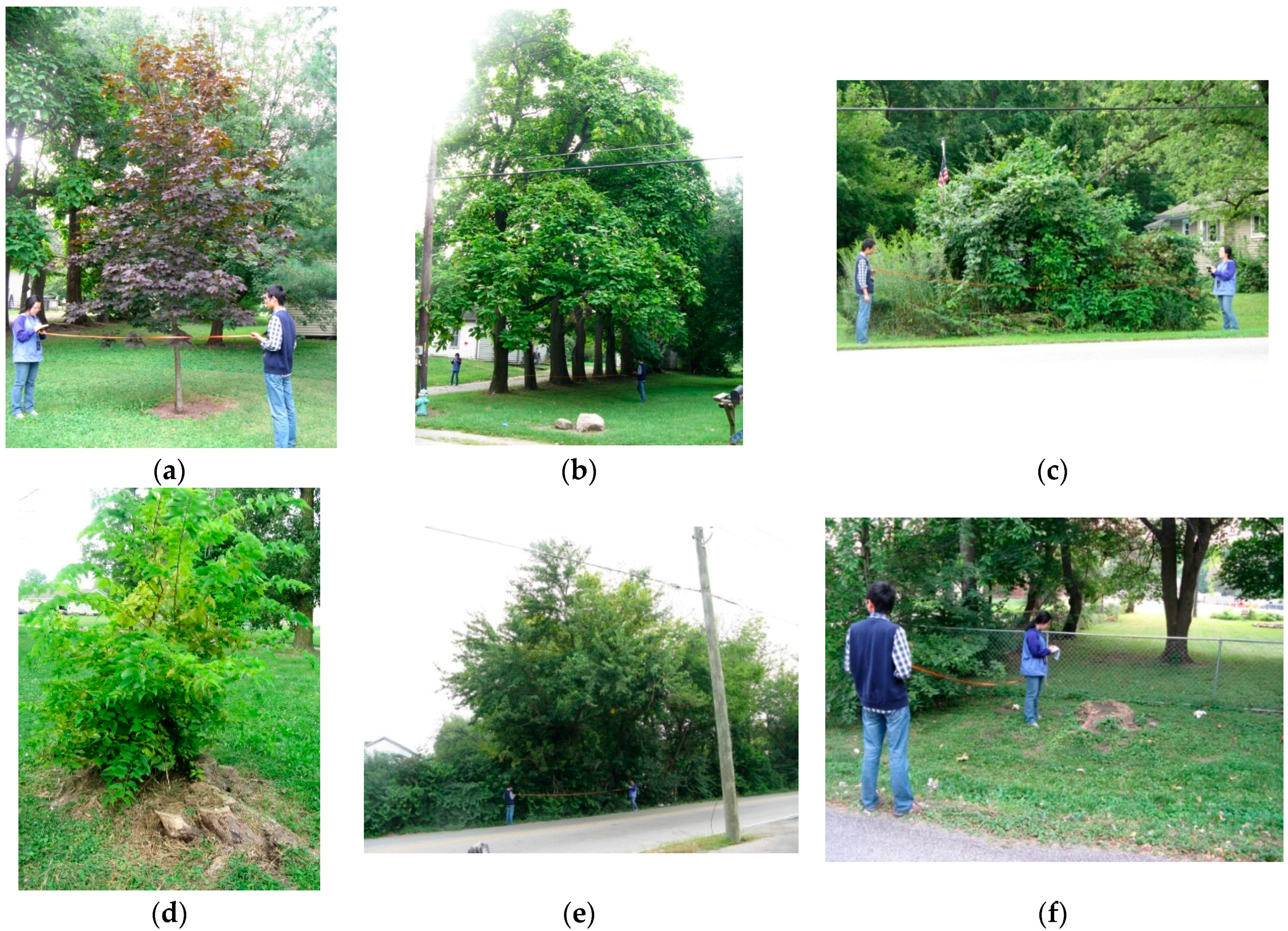
The individual tree segmentation is a key step in the process of estimating tree frontal areas. The currently available methods developed in agriculture and forest areas, such as the bottom–up approach (Lu et al., 2014), top–down method (Li et al., 2012), and watershed algorithm (Chen et al., 2006; Alonzo et al., 2014), are promising for dealing with stand-alone trees (Figure 7a) and segmenting similar species (Figure 7b). However, with the mixture of tree species and shrub (Figure 7c,d), these methods have limitations. Better segmentation techniques and tree inventory with shrub information may be helpful to differentiate trees and shrubs. Further, human intervention and maintenance was another factor that affected tree growth in urban areas. Tree removal (Figure 7e) and new growing after removal (Figure 7f) may not be documented in a tree inventory or not match the LiDAR data. Field work and frequently updated tree inventory data are important for validation.
Intensity value was used to differentiate trunks and branches with leaves because it determined by surface reflectance, which is related to surface texture and roughness [27]. A threshold of greater and equal to 35 was used in [27] to detect the trunks and branches. In our study, we found that a threshold of smaller and equal to 30 yielded better results. The difference in intensity value is due to from various texture and roughness of trunks, branches, and leaves from different tree species. The proper choices of threshold vary by tree species and regions.
The Terrestrial LiDAR data was collected in the fall season, September 2013. Trees were basically leaf-on then. Since most of the trees were deciduous, tree frontal areas decreased in winter, making them less effective as wind blocks than in fall and summer. The conifers’ frontal areas did not change much in winter, and they provided a wind block year round. Therefore, research of the seasonal changes of tree frontal area for deciduous trees is desirable.
The category of dominant, intermediate, and understory of trees were based on the mature size rather than young trees. Therefore, the dominant category may contain younger trees in various growing stages. In addition, some tree types, such as Autumn Olive, were classified as a shrub to small tree, typically 3.5 m in height. As a shrub it would be understory, but as a small tree, 3.5 m would be intermediate. Therefore, field investigation and hard rules would be helpful to improve the categorization of trees.
In this study, frontal area was extracted from Terrestrial LiDAR data, and other geometric variables, except DBH, were also from Terrestrial LiDAR data. This may partly explain the very high R2. Data from other sources, for instance, aerial LiDAR and tree canopy cover from NLCD needs to be tested in future research. In addition, the tree inventory data only included trees on public land, and the LiDAR extracts were joined to the tree inventory. Therefore, the frontal area can only represent the trees public land, and not every tree in a 30 m pixel was represented. This might be the reason that the NDVI and tree canopy cover did not show high correlation (0.27) with tree frontal area. More research is needed to represent all trees in a pixel. Potentially, this technique can now be used and extrapolated to all trees. The LiDAR data could quickly be used to calculate wind resistance for a larger area and to relate to NDVI and tree canopy data.

5. Conclusions

The tree frontal area is one of the most influential factors in urban surface roughness estimation in micrometeorological studies. This study presents the first attempt to estimate the frontal areas of trees in an urban area using Terrestrial LiDAR, tree inventory data, NDVI, and NLCD tree canopy cover. We estimated the frontal area of individual trees as well as per 30 m pixel. Instead of using conventional methods based on LULC types or geometrical models, Terrestrial LiDAR data offered great potentials to extract true and timely individual tree frontal areas in urban settings. Furthermore, this study found the high correlation between tree frontal area and tree crown base area, which indicated that NLCD tree canopy cover data can be useful in tree frontal area estimation. The results of regression modeling indicated that extra information from tree inventory may not be helpful in the calculation of tree frontal area, but it was useful in validation and explanation of the results. A proper tree categorization according to the vertical air resistance, e.g., height and canopy density, was effective to reduce the RMSE in tree frontal area estimation. Geometric parameters, such as height, crown base height, and crown base area extractable from airborne LiDAR, may also be sufficient for tree frontal area estimation in the areas where Terrestrial LiDAR is not available.

Acknowledgments

We acknowledge Jim Stout, the former Program Manager of Indianapolis Mapping and Geographic Infrastructure System for providing Terrestrial LiDAR data, Bill Kincius, Manager of Urban Forestry, Department of Public Works, the City of Indianapolis for providing tree inventory data, Robert Neary, Staff Geographer and Project Manager from Keep Indianapolis Beautiful, Inc. (Indianapolis, IN, USA.) for valuable discussion on urban tree growing, and George Vosselman from University of Twente, The Netherland, for providing Point Cloud Mapper. We acknowledge Peng Fu and Yuanfan Zheng from Center for Urban Environmental Change, Indiana State University, for their help in the field work. We also acknowledge the constructive comments from four anonymous reviewers and efficient correspondence from editors.

Author Contributions

Yitong Jiang and Qihao Weng co-designed the study and methods. Steven Baker contributed in writing scripts for Terrestrial LiDAR data, and James H. Speer contributed in tree crown density classification. Yitong Jiang wrote a draft manuscript, Qihao Weng and James H. Speer revised the manuscript.

Conflicts of Interest

The authors declare no conflict of interest.

Appendix A

Table A1. The detailed suggested tree categories based on the degree of the resistance to air flow based on tree stature (understory, intermediate, or dominant) and crown density (broad or sparse).
Tree NameGenusUnderstory/Intermediate/DominantBroad/Sparse CanopySuggested Category
Honeysuckle, spp.LoniceraUS1
DogwoodCornusUS1
RedbudCercisUS1
Arborvitae spp.ThujaUB2
Autumn OliveElaeagnusUB2
Mulberry, spp.MorusUB2
Red MulberryMorusUB2
Russian-OliveElaeagnusUB2
SmoketreeCotinusUB2
Staghorn SumacRhusUB2
White MulberryMorusUB2
AppleMalusUB2
LilacSyringaUB2
ServiceberryAmelanchierUB2
SumacSumacUB2
ZelkovaZelkovaUB2
American SycamorePlatanusIS3
IronwoodOstryaIS3
GinkgoGinkgoIS3
HawthornCrataegusIS3
LocustRobiniaIS3
PearPyrusIS3
Plane treePlatanusIS3
PoplarPoplarIS3
Black CherryPrunusIB4
Cherry, Japanese floweringPrunusIB4
Cherry, Plum, PeachPrunusIB4
Cherry, sweetPrunusIB4
ChokecherryPrunusIB4
Golden RaintreeKoelreuteriaIB4
Higan CherryPrunusIB4
MimosaAlbiziaIB4
Northern CatalpaCatalpaIB4
Osage-OrangeMacluraIB4
PersimmonDiospyrosIB4
plum, cherryPrunusIB4
YellowwoodPrunusIB4
BuckeyeAesculusIB4
MagnoliaMagnoliaIB4
PrunusPrunusIB4
SweetgumLiquidambarIB4
WillowSalixIB4
Ash, pumpkinFraxinusDB5
Kentucky CoffeetreeGymnocladusDS5
BirchBetulaDS5
American LindenTiliaDB6
Baldcypress ‘Shawnee Brave’TaxodiumDS6
BoxelderAcerDB6
Chancelleor LindenTiliaDB6
Eastern CottonwoodPopulusDS6
HackberryCeltisIB6
HorsechestnutAesculusDB6
PecanCaryaDB6
Silver LindenTiliaDB6
Tree-Of-HeavenAilanthusIB6
AshFraxinusDB6
BeechFagusDB6
ElmUlmusDB6
HickoryCaryaDB6
MapleAcerDB6
OakQuercusDB6
TupeloNyssaDB6
WalnutJuglansDB6
Dawn RedwoodMetasequoiaDB7
Douglas FirPseudotsugaDB7
White FirAbiesDB7
Conifer DB7
Note: the bold tree names were found in validation site, but not in calibration site.

References

  1. Weng, Q. Thermal infrared remote sensing for urban climate and environmental studies: Methods, applications, and trends. ISPRS J. Phtogramm. 2009, 64, 335–344. [Google Scholar] [CrossRef]
  2. Vancutsem, C.; Ceccato, P.; Dinku, T.; Connor, S.J. Evaluation of MODIS land surface temperature data to estimate air temperature in different ecosystems over Africa. Remote. Sens. Environ. 2010, 114, 449–465. [Google Scholar] [CrossRef]
  3. Ho, H.C.; Knudby, A.; Sirovyak, P.; Xu, Y.; Hodul, M.; Henderson, S.B. Mapping maximum urban air temperature on hot summer days. Remote. Sens. Environ. 2014, 154, 38–45. [Google Scholar] [CrossRef]
  4. Norman, J.M.; Kustas, W.P.; Humes, K.S. A two source approach for estimating soil and vegetation energy fluxes in observations of directional radiometric surface temperature. Agric. For. Meteorol. 1995, 77, 263–293. [Google Scholar] [CrossRef]
  5. Kato, S.; Yamaguchi, Y. Estimation of storage heat flux in an urban area using ASTER data. Remote. Sens. Environ. 2007, 110, 1–17. [Google Scholar] [CrossRef]
  6. Weng, Q.; Hu, X.; Quattrochi, D.A.; Liu, H. Assessing intra-urban surface energy fluxes using remotely sensed ASTER imagery and routine meteorological data: A case study in Indianapolis, U.S.A. IEEE J. Sel. Top. Appl. Earth Obs. Remote. Sens. 2013, 7, 4046–4057. [Google Scholar] [CrossRef]
  7. Grimmond, C.S.B.; Cleugh, H.A.; Oke, T.R. An objective urban heat storage model and its comparison with other schemes. Atmos. Environ. 1991, 25B, 311–326. [Google Scholar] [CrossRef]
  8. Stull, R.B. An Introduction to Boundary Layer Meteorology; Kluwer Academic Publisher: Dordrecht, The Netherlands, 1988. [Google Scholar]
  9. Grimmond, C.S.B.; Oke, T.R. Aerodynamic properties of urban areas derived from analysis of surfaces form. J. Appl. Meteorol. 1999, 38, 1262–1292. [Google Scholar] [CrossRef]
  10. Paul-Limoges, E.; Christen, A.; Coops, N.C.; Black, T.A.; Trofymow, J.A. Estimation of aerodynamic roughness of a harvested Douglas-fir forest using airborne LiDAR. Remote. Sens. Environ. 2013, 136, 225–233. [Google Scholar] [CrossRef]
  11. Bottema, M. Urban roughness modelling in relation to pollutant dispersion. Atmos. Environ. 1997, 31, 3059–3075. [Google Scholar] [CrossRef]
  12. Raupach, M.R. Simplified expressions for vegetation roughness length and zero-plane displacement as functions of canopy height and area index. Bound.-Layer Meteorol. 1994, 71, 211–216. [Google Scholar] [CrossRef]
  13. Macdonald, R.W.; Griffiths, R.F.; Hall, D.J. An improved method for estimation of surface roughness of obstacle arrays. Atmos. Environ. 1998, 32, 1857–1864. [Google Scholar] [CrossRef]
  14. Burian, S.J.; Brown, M.J.; Linger, S.P. Morphological Analyses Using 3D Building Database: Los Angeles, California; Los Alamos National Laboratory: Los Angeles, CA, USA, 2002.
  15. Burian, S.J.; Han, W.S.; Brown, M.J. Morphological Analyses Using 3D Building Databases: Houston, Texas; Los Alamos National Laboratory: Los Angeles, CA, USA, 2003.
  16. Burian, S.J.; Han, W.S.; Brown, M.J. Morphological Analyses Using 3D Building Databases: Oklahoma City, Oklahoma; Los Alamos National Laboratory: Los Angeles, CA, USA, 2003.
  17. Antonarakis, A.S.; Richards, K.S.; Brasington, J.; Bithell, M. Leafless roughness of complex tree morphology using terrestrial LiDAR. Water Resour. Res. 2009, 45. [Google Scholar] [CrossRef]
  18. Vosselman, G.; Gorte, B.; Sithole, G.; Rabbani, T. Recognizing structure in laser scanner point clouds. Int. Arch. Photogramm. Remote. Sens. Spat. Inf. Sci. 2004, 46, 33–38. [Google Scholar]
  19. Lafarge, F.; Descombes, X.; Zerubia, J.; Pierrot-Deseilligny, M. Automatic building extraction from DEMs using an object approach and application to the 3D-city modeling. ISPRS J. Photogramm. 2008, 63, 365–381. [Google Scholar] [CrossRef] [Green Version]
  20. Zhou, Q. 3D Urban Modeling from City-Scale Aerial LiDAR Data; Doctoral Dissertation, University of South California: Los Angeles, CA, USA, 2012. [Google Scholar]
  21. Sun, S. Automatic 3D Building Detection and Modeling from Airborne LiDAR Point Clouds; Rochester Institute of Technology: Rochester, NY, USA, 2013. [Google Scholar]
  22. Sun, S.; Salvaggio, C. Aerial 3D building detection and modeling from Airborne LiDAR point clouds. IEEE J. Sel. Top. Appl. 2013, 6, 1440–1449. [Google Scholar] [CrossRef]
  23. Rutzinger, M.; Pratihast, A.K.; Oude Elberink, S.; Vosselman, G. Detection and modeling of 3D trees from mobile laser scanning data. Int. Arch. Photogramm. Remote. Sens. Spat. Inf. Sci. 2010, XXXVIII, 520–525. [Google Scholar]
  24. Chen, Q.; Baldocchi, D.; Gong, P.; Kelly, M. Isolating individual trees in a Savanna woodland using small footprint LiDAR data. Photogramm. Eng. Remote. Sens. 2006, 72, 923–932. [Google Scholar] [CrossRef]
  25. Alonzo, M.; Bookhagen, B.; Roberts, D.A. Urban tree species mapping using hyperspectral and LiDAR data fusion. Remote. Sens. Environ. 2014, 148, 70–83. [Google Scholar] [CrossRef]
  26. Li, W.; Guo, Q.; Jakubowski, M.K.; Kelly, M. A new method for segmenting individual trees from the LiDAR point cloud. Photogramm. Eng. Remote. Sens. 2012, 78, 75–84. [Google Scholar] [CrossRef]
  27. Lu, X.; Guo, Q.; Li, W.; Flanagan, J. A bottom-up approach to segment individual deciduous trees using leaf-off LiDAR point cloud data. ISPRS J. Phtogramm. 2014, 94, 1–12. [Google Scholar] [CrossRef]
  28. Jennings, S.B.; Brown, N.D.; Sheil, D. Assessing forest canopies and understorey illumination: Canopy closure, canopy cover and other measures. Forestry 1999, 71, 59–73. [Google Scholar] [CrossRef]
  29. Fahey, R.T.; Bialecki, M.B.; Carter, D.R. Tree growth and resilience to extreme drought across an urban land-use gradient. Arboric. Urban For. 2013, 39, 279–285. [Google Scholar]
  30. Wu, B.; Yu, B.; Yue, W.; Shu, S.; Tan, W.; Hu, C.; Huang, Y.; Wu, J.; Liu, H.A. Voxel-based method for automated identification and morphological parameters estimation of individual street trees from mobile laser scanning data. Remote. Sens. 2013, 5, 584–611. [Google Scholar] [CrossRef]
  31. Burnham, K.P.; Anderson, D.R. Model Selection and Multimodel Inference: A practical Information-Theoretic Approach, 2nd ed.; Springer-Verlag: New York, NY, USA, 2002. [Google Scholar]
Figure 1. The location of the study area, Marion County, Indiana, USA, and the nine townships in Marion County.
Remotesensing 08 00401 g001
Figure 2. The flowchart of estimating tree frontal areas in urban areas.
Remotesensing 08 00401 g002
Figure 3. The calibration and validation sites.
Remotesensing 08 00401 g003
Figure 4. Demonstrating the process of individual tree segmentation: (a) the original Terrestrial LiDAR tile; (b) ground removal; (c) surface growing; (d) planar removal; (e) connect components; (f) tree detection; (g) trunk and branch building for individual tree segmentation; and (h) allocating the rest of the points.
Remotesensing 08 00401 g004
Figure 5. (a) Three transects for validation and (b) validation of field observed tree width (along N-S direction) versus LiDAR Estimates.
Remotesensing 08 00401 g005aRemotesensing 08 00401 g005b
Figure 6. R2 (a) and RMSE (b) of three models on seven tree categories.
Remotesensing 08 00401 g006
Figure 7. Stand-alone trees (a) and stands with similar species (b) segment easily; trees with vine and shrub (c,d) are hard to be segmented; Trees may have changed form from previous data collecting because of removal (e) and growing after removal (f).
Remotesensing 08 00401 g007
Table 1. The suggested tree categories based on the degree of the resistance to air flow based on tree stature (understory, intermediate, or dominant) and crown density (broad or sparse).
Suggested CategoryUnderstory/Intermediate /DominantBroad/Sparse CanopyExamples of Trees
1USHoneysuckle, Dogwood, Redbud
2UBArborvitae, Autumn Olive, Mulberry
3ISAmerican Sycamore, Poplar, Ginkgo
4IBBlack Cherry, Buckeye, Willow
5DBBirch, Kentucky Coffeetree
6DSAsh, Beech, Elm, Maple, Walnut
7DBDawn Redwood, Conifer, Douglas Fir
Table 2. Correlation between frontal area from TLiDAR and the independent variables.
Independent VariablesPearson CorrelationData Source
Sum DBH0.519Tree Inventory
# of trees with two abnormal diagnoses0.624Tree Inventory
# of trees in poor condition0.609Tree Inventory
# of trees performed large tree clean0.518Tree Inventory
# of trees with utility maintenance 0.608Tree Inventory
# of tree with sidewalk heaved <3/4 inch0.661Tree Inventory
# of trees in Single-family residential land0.568Tree Inventory
# of trees with <4 in defect0.569Tree Inventory
Sum Crown Base Area0.991Terrestrial LiDAR
Sum Height0.853Terrestrial LiDAR
Sum width (EW length)0.922Terrestrial LiDAR
Sum width (NS length)0.901Terrestrial LiDAR
Note: the independent variables in this table are the ones with a correlation greater than 0.5. # = number.