Abstract
Near surface air temperature (Ta) is one of the most critical variables in climatology, hydrology, epidemiology, and environmental health. In situ measurements are not efficient for characterizing spatially heterogeneous Ta, while remote sensing is a powerful tool to break this limitation. This study proposes a mapping framework for daily mean Ta using an enhanced empirical regression method based on remote sensing data. It differs from previous studies in three aspects. First, nighttime light data is introduced as a predictor (besides land surface temperature, normalized difference vegetation index, impervious surface area, black sky albedo, normalized difference water index, elevation, and duration of daylight) considering the urbanization-induced Ta increase over a large area. Second, independent components are extracted using principal component analysis considering the correlations among the above predictors. Third, a composite sinusoidal coefficient regression is developed considering the dynamic Ta-predictor relationship. This method was performed at 333 weather stations in China during 2001–2012. Evaluation shows overall mean error of −0.01 K, root mean square error (RMSE) of 2.53 K, correlation coefficient (R2) of 0.96, and average uncertainty of 0.21 K. Model inter-comparison shows that this method outperforms six additional empirical regressions that have not incorporated nighttime light data or considered predictor independence or coefficient dynamics (by 0.18–2.60 K in RMSE and 0.00–0.15 in R2).
1. Introduction
Near-surface air temperature (Ta), defined as the air temperature 2 m above the land surface [1], is one of the most critical variables in climatology [2], hydrology [3], epidemiology [4], and environmental health [2]. Ta is traditionally measured at weather stations. They provide highly frequent measurements with long-term records but are not efficient for characterizing spatial heterogeneities due to their low sampling densities [5,6], particularly over urban and mountainous areas, where climatic effects can be fairly strong.
Remote sensing, alternatively, provides a greatly important and valuable source of information that can be used to estimate spatially continuous Ta. The previous studies can be grouped into two categories: atmosphere-based and land-based. The former retrieves air temperature profiles over a wide coverage from atmospheric infrared radiation obtained by GOES [7], AIRS [8], MODIS [9], etc. The spatial resolution of the retrieved Ta is rather coarse (typically several to tens or hundreds of kilometers), and the accuracy is sometimes lower than 10 K [10].
The land-based studies commonly employ physical or statistical methods. The physical method is based on the energy balance dynamics, i.e., the sum of incoming net radiation and anthropogenic heat fluxes equals the sum of sensible, latent, and soil heat fluxes. The sensible and latent heat fluxes are transformed into a function of surface-air temperature differences and Ta is then derived by solving the energy balance equation [11]. The accuracy is generally 1–3 K [12]. This method has a solid physical background and is useful for exploring the essence of Ta formation and variation from an energy balance perspective. Nonetheless, it is not frequently used due to the complexity of the model [13].
The statistical method, on the other hand, is much simpler in practical use, including the geostatistical method, the temperature/vegetation index (TVX) method, and the empirical regression method. The geostatistical method often integrates remotely sensed land surface temperature (LST) with spatial interpolators, typically elevation, to estimate Ta from discrete sites using techniques such as kriging/co-kriging [14,15], spatial regression kriging [16], and geographically weighted regression [17]. The accuracy ranges from about 1 to 6 K. The remote sensing-based geostatistical method shows better estimates than the conventional regression method [14,17]. However, it is largely dependent on the arbitrary locations of weather stations [18,19].
The TVX method assumes that the bulk temperature of a fully vegetated canopy approximates the air temperature within the canopy, and Ta is thus predicted based on the TVX correlation and the estimated vegetation response of indefinitely thick canopy [20]. The accuracy is around 2–5 K [12]. This method requires no external data source beyond remotely sensed surface temperature and vegetation responses. However, it greatly relies on the negative TVX correlation built within a sample window [1,20], suggesting probable unstableness with varying soil moisture and window size and unsuitableness in winter, at night, and over urban, snow, ice, and water surfaces [20,21]. Moreover, the estimated Ta may have a strong spatial autocorrelation due to the moving window calculation [22].
The empirical regression method establishes a relationship of Ta with predictors, and then extends the relationship to surfaces with known predictors but unobserved Ta. It has two major parts: predictors and regression tools. Previous studies have adopted biophysical, geometrical, geographical and meteorological predictors, such as LST [6], normalized difference vegetation index (NDVI) [23], albedo [13], impervious surface area (ISA) [24], sky view factor (SVF) [1], normalized difference water index (NDWI) [1], elevation [25], and solar radiation [26]. Among them, LST and elevation are the most powerful ones [13]. The regression tools include linear regression [6,23,27], neural network [28], support vector machine [1], regression tree [26], etc. The regression method generally performs well (an accuracy of around 1–4 K) when training samples are appropriate [29]. The empirical regression method has simpler operability compared to the physical method, better robustness against weather station locations compared to the geostatistical method, and wider applicability on different covers compared to the TVX method.
However, the remote sensing-based regression method has typically focused on Ta mapping over non-urban areas [6,30,31]. With rapid urban expansion, an increasing number of weather stations have been newly installed in urban areas [32,33] and many previously rural weather stations have now been surrounded by urban surfaces [34]. Therefore, to better estimate Ta over a large area with urban, suburban and rural weather stations all together, it is necessary to take into account the urbanization impact. A few studies [1,35,36] have recently attempted to estimate Ta incorporating urban features such as ISA and SVF, and yet the considerable difference in anthropogenic heat caused by human activities (in sectors such as transportation, buildings, and human metabolism [37]) has not been accounted for over large regions. Previous studies using climate or meteorological models [38,39] have shown that anthropogenic heat is an important heating source to warm Ta [40] by 2 K or more [41]. Nevertheless, it is challenging to explicitly quantify spatio-temporal anthropogenic heat release across a wide area considering that it usually requires accessible and appropriate data from local agencies and institutions [42]. Also, energy balance-based quantification with remote sensing data is inapplicable and instable due to the spatio-temporal Ta that is to be estimated [43]. Alternatively, nighttime light data from DMSP/OLS were used by Chen et al. (2012) to approximate anthropogenic heat flux over entire China from 1992 to 2009 based on their strong linear correlation (correlation coefficient R2 > 0.9) [44]. Therefore, nighttime light data is possibly a supplement to the current predictor pool for accounting for the impact of anthropogenic heat to some extent.
Moreover, many previous regressions have adopted multiple predictors while neglecting their correlations [23,24], which leads to inflated parameter variances, instable coefficient estimates, and consequently biased Ta predictions [45]. Finally, the relationship between Ta and most predictors varies with time [35], and yet the regression coefficients have commonly been regarded as temporally stationary and uniformly determined through the whole period of time. One notable study to derive dynamic coefficients is provided by Good (2015) using temporally moving window regression [35].
This study presents a mapping framework for daily mean Ta using an enhanced empirical regression method based on remote sensing data. It differs from previous studies in that satellite-derived nighttime light data is introduced for the first time as one of the predictors to account for anthropogenic heat, and independent components are extracted from the multiple predictors before a time-varying coefficient regression modeled by composite sinusoidal functions is performed. Ta was estimated at 333 weather stations in China during 2001–2012 and then evaluated according to cross-validation, uncertainty analysis, and model inter-comparison.
The primary objectives of this study are three-fold. First, this study aims to develop a simple and practical method that improves the accuracy of Ta estimation and can be easily followed for other applications. Second, this study attempts to introduce the idea of using nighttime light data for Ta estimation and inspire others to further explore the relationship between the nighttime light data and Ta. Finally, this study provides a framework of using times series of multiple variables to estimate spatio-temporal Ta so that other meteorological variables can also be estimated under the similar framework.
2. Study Area and Data
2.1. Study Area and Meteorological Data
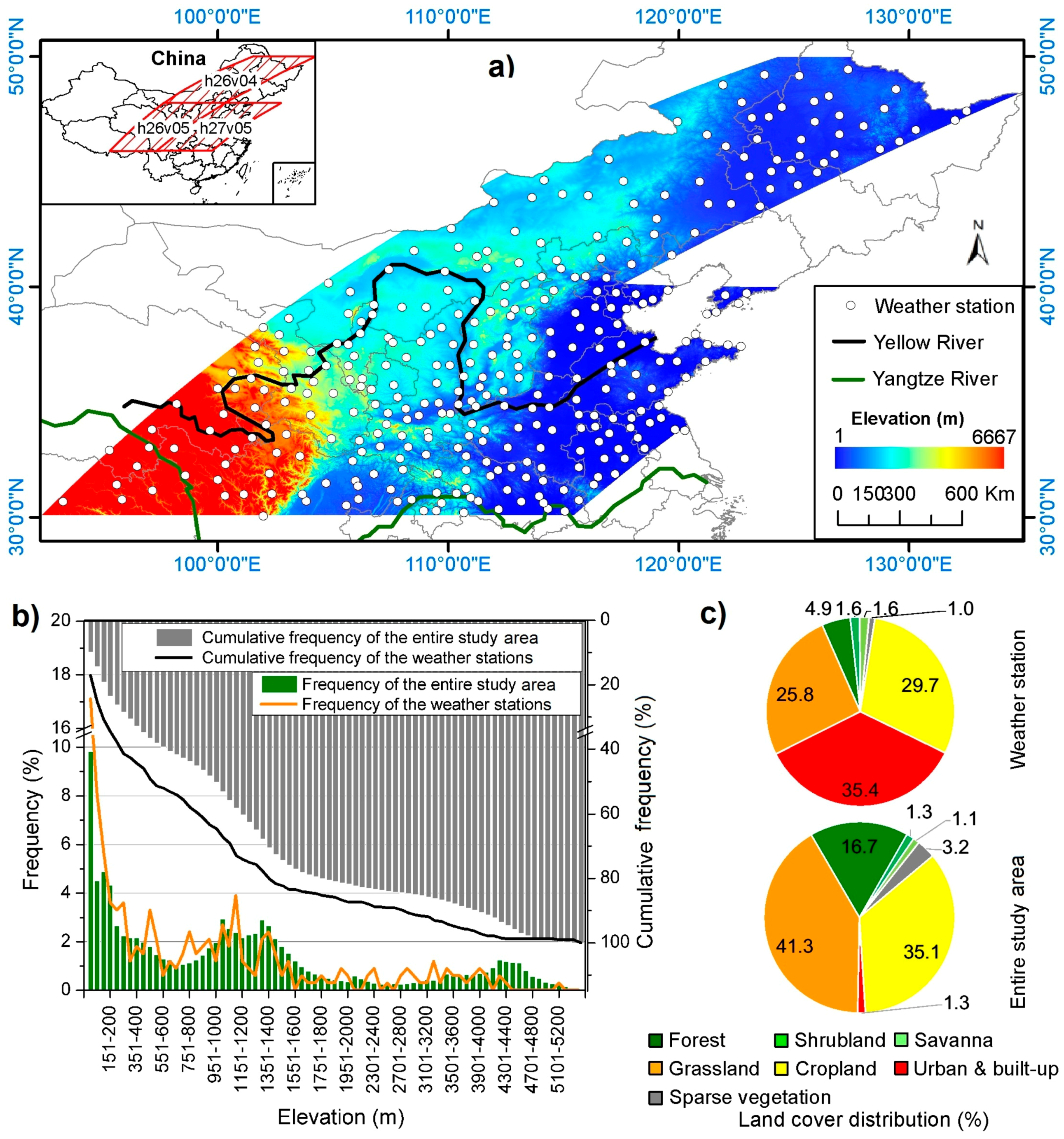
The study area (Figure 1a) corresponds to three MODIS sinusoidal tiles (i.e., h26v04, h26v05 and h27v05), covering an area of approximately 4.32 million km2 (30–50° N, 93–136° E) in China. The elevation (Figure 1a,b), ranging from 1 to 6667 m, forms a high western but low eastern terrain (also called the three-step ladder topography) [46]: the highest step is the Qinghai–Tibet Plateau with an average elevation of more than 4000 m and alpine highland climate; the medium step includes basins (e.g., Sichuan Basin) and plateaus (e.g., Loess Plateau) at 1000–2000 m elevations; and the lowest step is mainly plain (e.g., North China Plain) at elevations of 500 m or less. The medium and lowest levels exhibit temperate monsoon climate in the north and subtropical monsoon climate in the south. The main land covers are grasslands (41.3%), croplands (35.1%), and forest (16.7%); sparse vegetation, urban and built-up land, shrubland, and savanna cover the rest (6.9%) of the area (Figure 1c according to the yearly MODIS land cover product in 2012). The study area crosses 13 provinces in China (Figure 1a), with population ranging from 3 to 96 million in each province (according to the tabulation on the 2010 population census of China).

Figure 1.
General view of the study area and weather stations: (a) spatial view; (b) statistics of elevation; (c) statistics of land cover. The elevation and land cover data were obtained from GTOPO30 digital elevation model (DEM) and yearly MODIS land cover product (MCD13Q1) in 2012, respectively.
A total of 333 discrete weather stations are distributed across the study area (Figure 1a). More weather stations (~50%) are in the lower elevation regions (<500 m) and fewer (~3%) are in the higher elevation regions (>4000 m), as shown in Figure 1b, highlighting the necessity of providing Ta estimates in the regions with sparsely-distributed stations. The weather stations are primarily located over urban and built-up lands (35.4%), croplands (29.7%), and grasslands (25.8%), which together are rather representative (60%) of the study area considering their similar distributions over grasslands and croplands (Figure 1c). On the other hand, weather stations “over”-represent the urban and built-up lands, suggesting the importance of incorporating urbanization impacts for Ta estimation. Daily mean Ta values measured at these stations between 2001 and 2012 were collected from the China Meteorological Data Sharing Service System (http://cdc.nmic.cn), where Ta values with a quality flag of “fault,” “unobserved,” or “uncontrolled” were eliminated.
2.2. Spatio-Temporal Predictors
Eight variables (seven commonly used plus one never used) over the study area during the 2001–2012 period were used as predictors for Ta estimation (Table 1): LST, NDVI, ISA, black-sky albedo (BSA), NDWI, nighttime stable light (NSL), elevation (ELV), and duration of daylight (DDL). LST, NDVI, and BSA were directly collected from MODIS products (NASA’s EOSDIS, https://earthdata.nasa.gov/), while ISA and NDWI were further derived from the NDVI and BSA products. MODIS data were chosen mainly because they provided large coverage, high temporal resolution, a series of land surface products, and easy public access. NSL was obtained from DMSP/OLS (NOAA NCEI, http://www.ngdc.noaa.gov) considering its close correlation with anthropogenic heat release [47], ELV was obtained from GTOPO30 (USGS, https://lta.cr.usgs.gov/), and DDL, a substitute for solar radiation considering their significant relationship [48], was calculated according to the latitude of a given location and the day of a year.

Table 1.
Predictors used for Ta estimation.
2.2.1. LST
Daily LST product acquired by Terra at ~22:30 with a spatial resolution of 1 km (MOD11A1 in version 5) was obtained. It is retrieved using a generalized split-window algorithm [49], resulting in an accuracy of 2 K in most cases [50]. However, the error can be markedly increased due to systematic anomalies (e.g., due to the MODIS optical leak correction error inducing anomalously high values at the end of scan lines) [29], large emissivity uncertainties (e.g., in arid and semi-arid areas) [51], and complex atmospheric conditions (e.g., clouds and heavy aerosols) [52].
Therefore, the following procedures were performed to eliminate low quality data. First, LSTs with sensor zenith angles of <11° or >130° were considered to suffer from a significant error from the optical leak correction and thus excluded. Then, LSTs flagged with “average emissivity error ≤0.04 (or >0.04)” or “average LST error >3 K” were eliminated. Finally, abnormally low LSTs, determined by histogram-based quartile statistics [53], were probably caused by undetected clouds and thus filtered out. In this study, Terra nighttime LST, instead of Aqua and/or daytime LST, was chosen because it is more stable and accurate [54,55] and has a weaker angular effect [56] and a larger number of valid pixels [57].
2.2.2. NDVI and ISA
A 16-day composite NDVI product acquired by Terra at ~10:30 with a spatial resolution of 250 m (MOD13Q1) was collected. It adopts the maximum/averaged NDVI value in the case of clouds/cloud-free to represent the entire 16-day period, where the daily NDVI is determined by atmospherically corrected red and near-infrared reflectance at a 250-m resolution (MOD09GQ). Pixels flagged with “lowest quality,” “quality so low that it is not useful,” “L1B data faulty,” or “not useful for any other reason/not processed” were eliminated.
ISA was derived year by year using a temporal mixture analysis of the annual NDVI time series (proposed by Yang et al. (2012) [58]), resulting in a temporal resolution of one year and a spatial resolution of 250 m. The fundamental assumption of this process is that the NDVI series can be regarded as linear mixtures of temporal profiles of endmember NDVI series. In detail, the NDVI series of each pixel were rearranged from high to low values and six maximums were extracted; then principal component analysis (PCA) was conducted on the six maximum NDVI series and three endmembers (i.e., forest, crops, and impervious surface) were determined; and finally, the NDVI series of each pixel were linearly unmixed according to the endmember NDVI series and the endmember fractions (including ISA) were obtained.
2.2.3. BSA and NDWI
Terra/Aqua combined 16-day composite albedo product with a spatial resolution of 500 m (MCD43A3) was collected. It is generated from Terra and Aqua daily reflectance (MOD09GA and MYD09GA) during a 16-day period using the 16-day anisotropy model (MCD43A1). MCD43A3 contains BSA (i.e., directional hemispherical reflectance) and white-sky albedo (i.e., bi-hemispherical reflectance) for seven narrowbands and visible, near-infrared, and shortwave broadbands. Given that BSA and white-sky albedo are almost linearly correlated [47] and total solar energy reflected by the surface is commonly characterized by the shortwave broadband [59], BSA-shortwave was extracted and the pixels flagged with “processed, good quality” or “magnitude inversion [numobs ≥ 7]” were used.
NDWI, an indicator of water content [60], was calculated from BSA for near- and mid- infrared bands (i.e., ), generating spatial and temporal resolutions of 16-day and 500 m, respectively.
2.2.4. NSL
DMSP/OLS stable light data (NSL), an annual composite of cloud-free nighttime lights with a grid cell of 30 arc seconds, was used. NSL covers nighttime lights from urban, suburban, and rural areas with persistent lighting and discards ephemeral events, such as fires [61]. Pixels outside the valid data range 1–63 were eliminated. Lacking on-board calibration and setting a constant gain, NSL time series obtained from different sensors (e.g., F15: 2000–2007, F16: 2004–2009, and F18: 2010–2012) are not directly comparable.
Therefore, an inter-calibration was performed following Elvidge et al. (2009) [62]. First, the city of Jixi in Heilongjiang Province was selected as the calibration area due to its stable socio-economic development, and NSL from satellite F16 in 2007 of the calibration area was chosen as the reference considering the highest cumulative value [61]. Then, a second-order regression was conducted between the reference data and the other dataset of the calibration area to eliminate inter-annual discrepancies [63], and the derived regression coefficients were further used to calibrate the NSL time series over the entire study area [63]. Finally, NSL from different satellites in the same year was averaged to keep continuity during the period.
2.2.5. ELV
GTOPO30, a digital elevation model (DEM) with a horizontal grid spacing of 30 arc seconds, was used. Eight sources of topographic information are used to derive GTOPO30 and the estimated accuracy is considered suitable for regional climate applications (http://webgis.wr.usgs.gov/globalgis/gtopo30/gtopo30.htm).
2.2.6. DDL
DDL was calculated by Equation (1) over the study area with the same spatial and temporal resolutions as LST [64]:
where is the latitude, and DOY is the day of year.
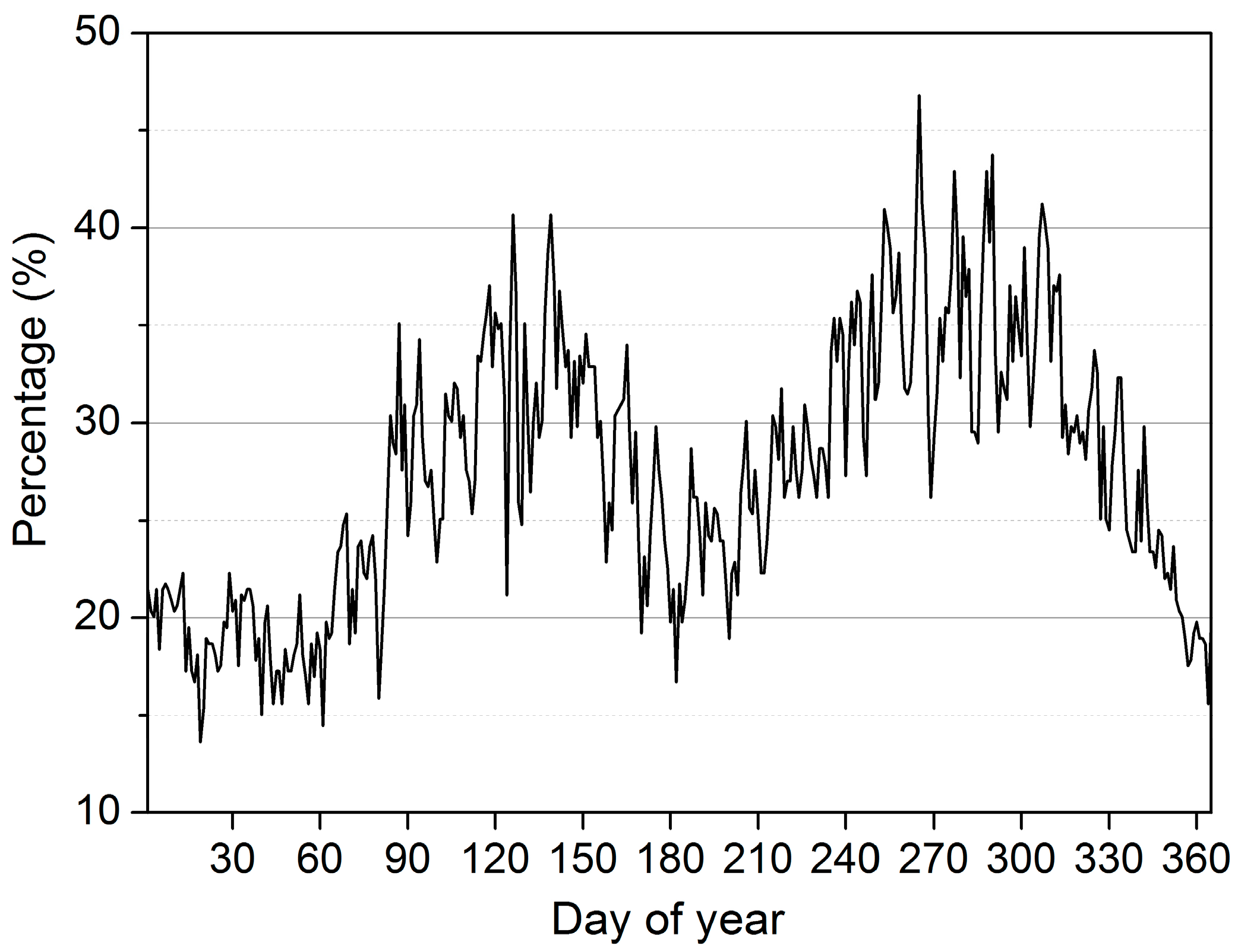
All of the above predictors were re-projected, co-registered, and then extracted for the weather station coordinates using the nearest neighbor method [29]. Any Ta-predictor correspondence with one or more invalid/unqualified values was excluded. Finally, a total of 433,108 Ta-predictor “pairs” were available for the following method over this study area between 2001 and 2012. They had a significant seasonality (Figure 2) that was mainly determined by the distribution of qualified MODIS/LSTs due to the clouds [57].

Figure 2.
Twelve-year and 333-station averaged daily distribution (as percentage) of qualified Ta-predictor “pairs.”
3. Methods
The overall modeling framework (Figure 3) contained three steps. Step 1: z-score standardization and PCA were used to extract independent components from the eight predictors (Section 3.1); Step 2: the obtained independent components were regressed against Ta collocated in both space and time following a time-varying coefficient scheme (Section 3.2); and Step 3: the derived regression coefficients were applied to available predictors for Ta estimation over the surfaces where weather stations were absent (Section 3.3). Three different experiments were conducted for model evaluation (Section 3.4): cross-validation, uncertainty analysis, and model inter-comparison. More detailed descriptions follow below.
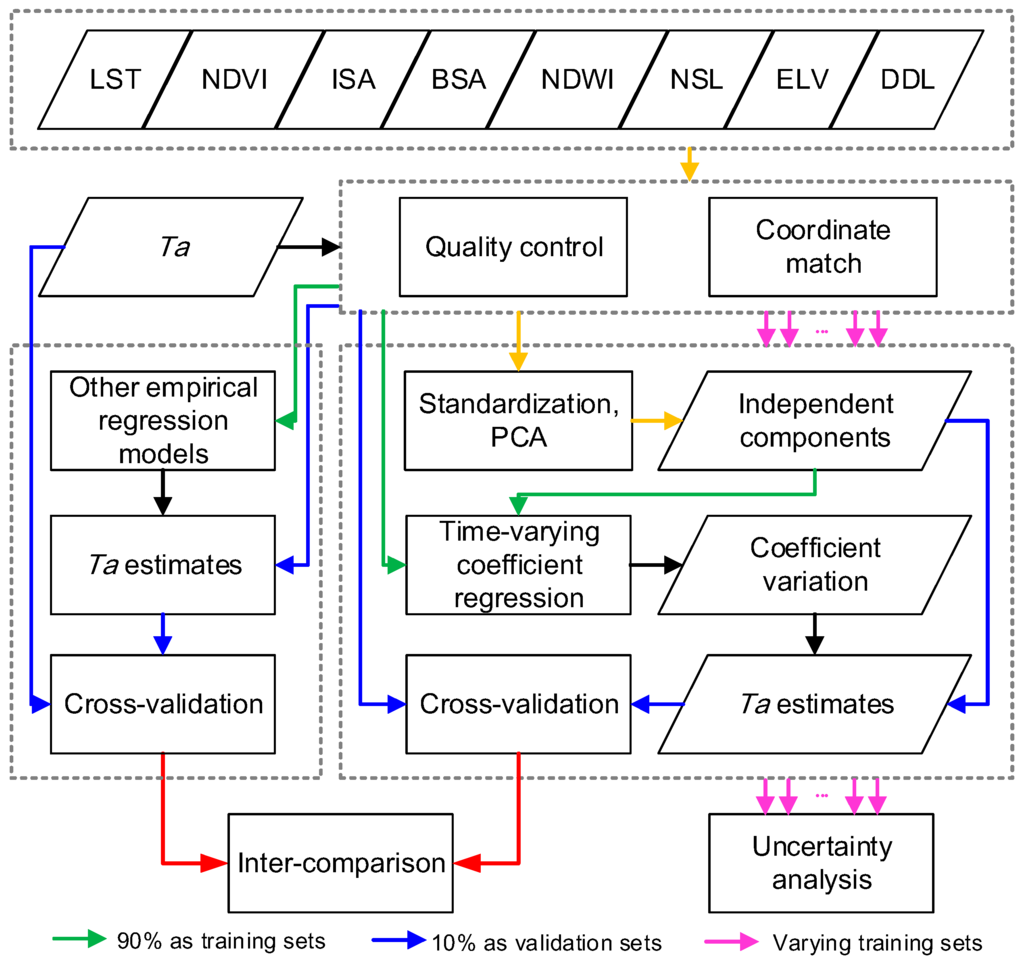
Figure 3.
Flowchart of methods.
3.1. Independent Component Extraction
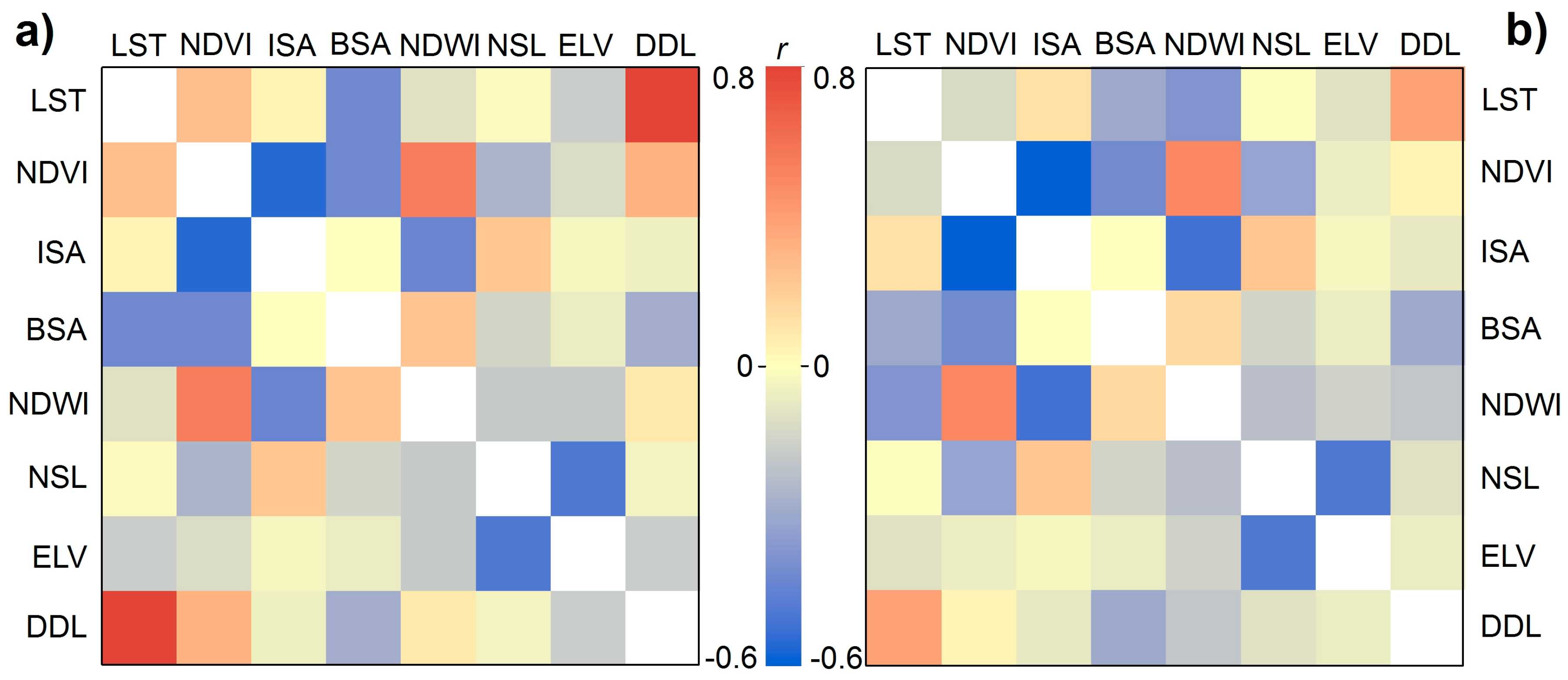
Collinearity among explanatory variables leads to series of problems in regression-based predictions, such as unreliable coefficients and predictions [45] as well as aggravated data redundancy and computational complexity. Therefore, the collinearity was first diagnosed using a pairwise Pearson’s linear correlation coefficient r, a major indicator of collinearity [45]. Considering that LST, NDVI, NDWI, and DDL annually vary in bell-shaped curves, their direct correlations are inflated and tend to be positive (e.g., r = 0.34 between LST and NDVI, Figure 4a). To reduce the influence of seasonality in time series, deseasonalization was separately conducted on LST, NDVI, NDWI and DDL by subtracting the monthly mean and then dividing by the monthly standard deviation [65] (Each year was divided into 12 months, and the mean value and standard deviation were calculated for each variable for each month during the 2001–2012 period.) Deseasonalization was not performed on the other four predictors because the BSA time series do not show a regular shaped seasonal pattern over different land covers and the ISA, NSL and ELV values are constant in a year for a given location. As a result (Figure 4b), r ranges from −0.6 to 0.5 after deseasonalization: that between NDVI and ISA is the highest (r = −0.6), and the positive/negative NDVI–NDWI, LST–DDL, NDWI–ISA, and NSL–ELV relationships are also remarkable (|r| > 0.4).

Figure 4.
Pairwise Pearson’s linear correlation coefficient r among the eight predictors (a) before and (b) after deseasonalization of the LST, NDVI, NDWI, and DDL time series.
Regarding this issue, z-score standardization and PCA were performed on the eight predictors. z-score standardization was used given the notably different dimensions and magnitudes of the eight predictors which cause the variance to be dominated by the predictor with a large scale during PCA [66]. Specifically, the time series of each predictor were separately standardized by subtracting the daily mean and then dividing by the daily standard deviation to achieve fair comparability [67] (The daily mean and standard deviation were calculated day by day from all observations of each variable during the 2001–2012 period.) PCA was chosen because it is a simple and commonly used orthogonal transformation that requires no parameter, removes variable correlations and thus reduces the collinearity [45]. Specifically, the eight standardized predictors were transformed into an orthogonal space, yielding a set of linearly uncorrelated components and their weights/coefficients [68]. Figure 5 shows that 86% of the variance was accounted for by the first four principal components (PC1–PC4), which were used as independents in the following regression. More components significantly increase the number of unknown parameters and thus the difficulty of solving the regression equations (Equation (5)), while fewer components include less spatio-temporal information, which may yield a lower accuracy.
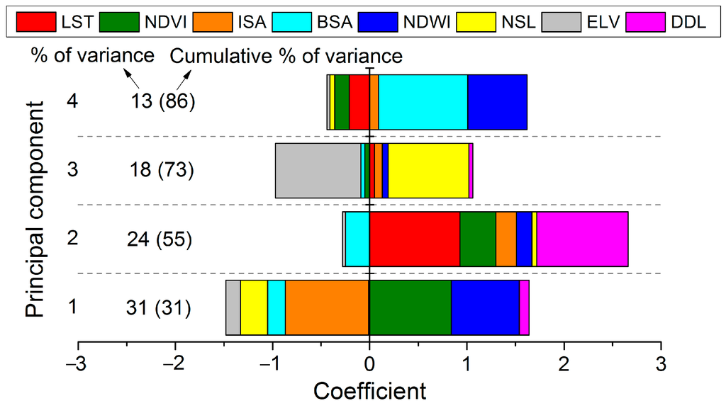
Figure 5.
PCA of the eight standardized predictors including the variance explained and the coefficient matrix (only the first four components are shown).
3.2. Time-Varying Coefficient Regression
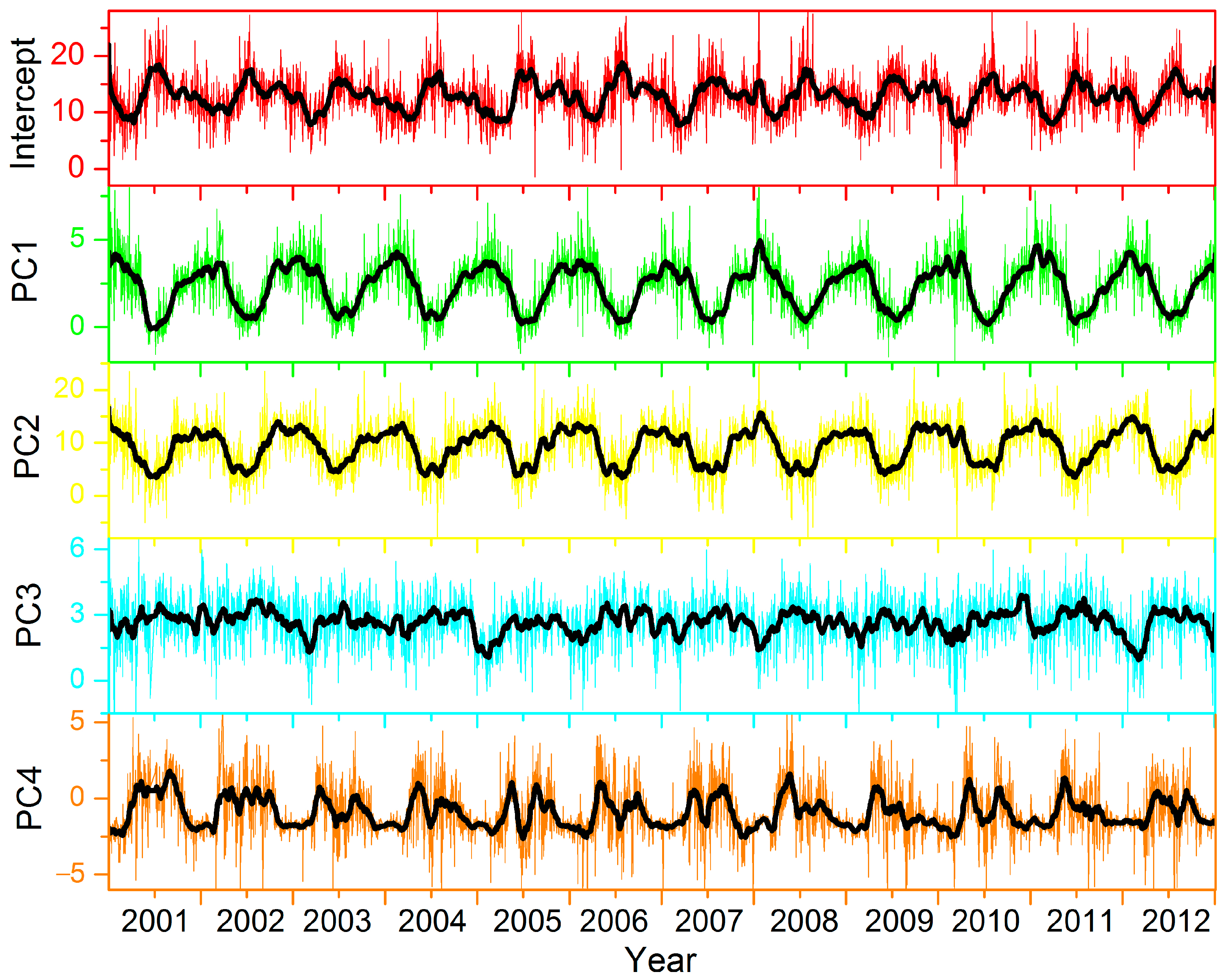
Linear regression between Ta and PC1-PC4 was performed day by day (Figure 6), showing significant temporal variations in the intercept and each of the regression coefficients, generally on seasonal and local timescales. Therefore, Ta was regressed against temporally and spatially collocated PCs using time-varying coefficients (Equation (2)) that were assumed to be smooth and modeled here as composite sinusoidal functions (Equations (3) and (4)):
with
where is Ta at site m on day n, is the time-varying intercept, is the time-varying slope of PC , is the PC value, L is the total number of PCs (i.e., 4 in this study), is the random error; is the mean value of , , and are the amplitude, frequency, and phase shift of the ith sine function of , respectively, and is the total number of the sine functions; similarly, , , , , and are the parameters of sine functions for .
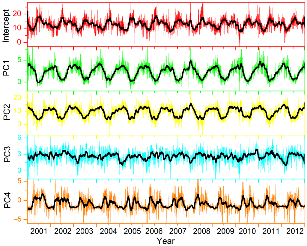
Figure 6.
Coefficients and intercept of the linear regression day by day between Ta and PC1–PC4. The thin lines are the daily results and the thick lines are the smoothed results by a 30-day moving window.
By including multiple sites and days, a set of equations was formulated as follows:
with
where M and N are the total numbers of weather stations and days included, respectively.
3.3. Spatio-Temporal Ta Estimation
The number of known Ta observations is . The number of unknown parameters (i.e., , , , , , , , , , and ) is . A Levenberg–Marquardt algorithm with a universal optimization scheme was applied to solve Equation (5). The derived coefficients were then applied back to the spatially collocated predictors across the entire study area and period to reconstruct spatio-temporal Ta according to Equations (2)–(4). The estimated Ta has a spatial resolution of 250 m and a temporal resolution of one day, while Ta is absent in the case of missing PCs/predictors due to the quality control.
3.4. Model Evaluation
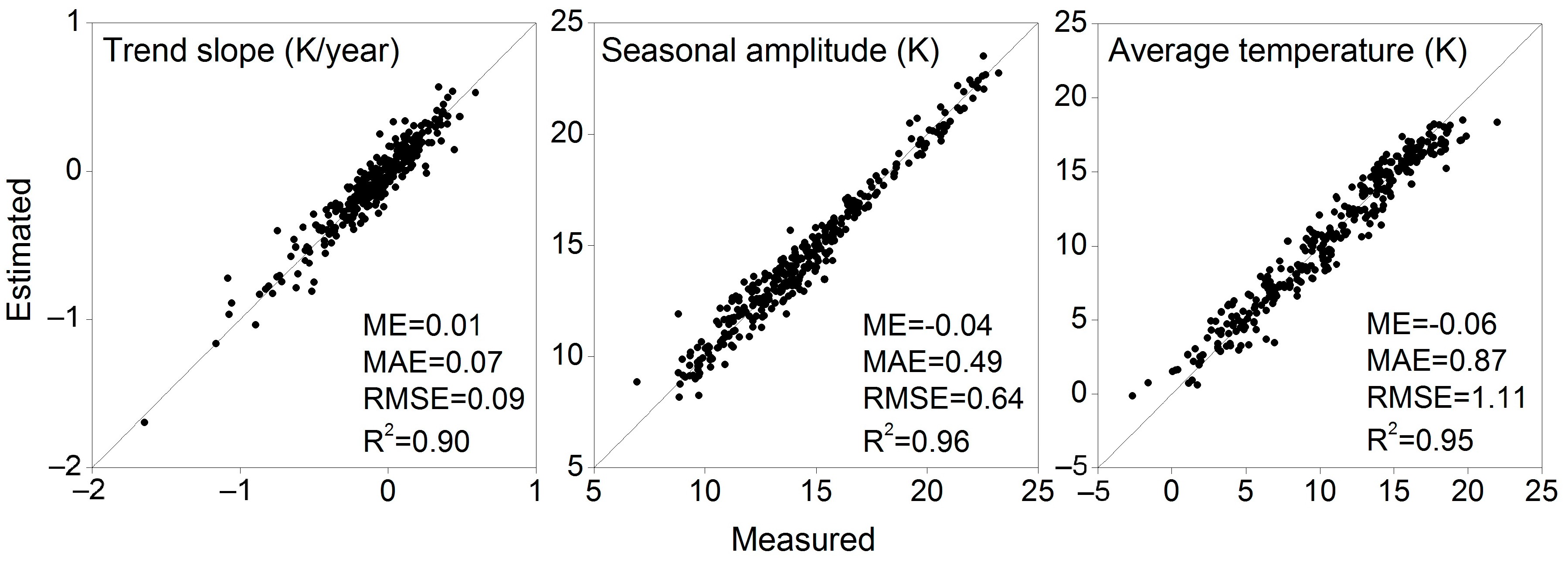
First, cross-validation was conducted by a leave-10%-out procedure. Specifically, we divided the study area into 12 subsets and randomly, in each subset, selected 90% of the collocated data as training sets, and then estimated Ta of the remaining 10% with the regression model parameterized by the selected 90%. This procedure was repeated 10 times in each subset (i.e., a total of 120 times in the study area). The root mean square error (RMSE), mean absolute error (MAE), mean error (ME), and correlation coefficient (R2) of the predicted Ta versus the measured Ta for each withheld weather station were calculated and then summarized across space (by land cover and site) and time (by year, season and month). To further evaluate the representation of temporal patterns by the predicted Ta, trend and seasonal decomposition [69] was performed on both the predicted and the measured Ta time series during the study period. The derived inter- and intra-annual variation parameters (mainly trend slope, seasonal amplitude and annual average temperature) were compared over each weather station.
Second, uncertainty analysis was performed using a jackknife-bootstrap procedure [29]. Specifically, a total of 120 different training sets were randomly selected to obtain regression parameters which were then used to estimate Ta at the same weather station on the same day. The standard deviation of all Ta estimates for a given station at a given time was defined as the absolute uncertainty. The spatio-temporal average uncertainty and the uncertainty statistics by land cover and weather station were calculated.
Finally, model inter-comparison was conducted to show the relative improvements of the proposed model ((6) in Figure 7). Specifically, six additional empirical regressions were used ((1)–(6) in Figure 7): (1) temporally stationary, linear regression with LST, (2) temporally stationary, multi-linear regression with the seven predictors (without NSL), (3) temporally stationary, multi-linear regression with the eight predictors, (4) time-varying coefficient regression with PC1–PC4 of the eight predictors using a 30-day moving window [35], (5) time-varying coefficient regression with the eight predictors using composite sinusoidal functions, and (6) time-varying coefficient regression with PC1–PC4 of the seven predictors (without NSL) using composite sinusoidal functions. The above cross-validation procedure was also conducted for each of these models and the average RMSE and R2 were calculated and compared with those from our proposed model.

Figure 7.
Models as comparisons ((1)–(6)) to the proposed one (7). PRE7: LST, NDVI, ISA, BSA, NDWI, ELV, and DDL.
4. Results
4.1. Spatial Patterns of Errors
Figure 8a shows the scatter plot between the measured and the estimated Ta. Overall, a good agreement was found between them given the mean slope of 0.95, intercept of 0.48 and ME of −0.01 K (R2 = 0.96, p < 0.05, Figure 8b). The overall RMSE is 2.53 K with the 2.5th/97.5th percentiles (Figure 8b).
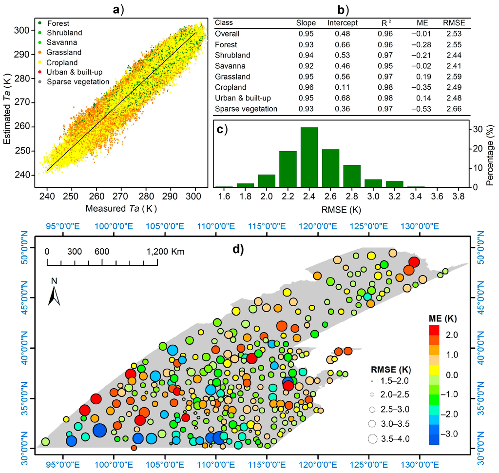
Figure 8.
Error between the estimated and the measured Ta: (a) scatter plot; (b) statistics of error by land cover; (c) histogram of average RMSE for weather stations; and (d) spatial distribution of RMSE and ME at weather stations.
Figure 8b shows the statistics of error by land cover. The biases between the estimated and the measured Ta are different among land covers (at a significance level of 0.05 according to t-test and F-test on their averages and variances). Yet the differences are not large in magnitude (0.03 in R2, 0.34 K in ME, and 0.25 K in RMSE), suggesting an independence of model performance against weather stations’ land covers.
Figure 8d displays the ME of each weather station; 2% show significant underestimation (−3.5 < ME < −2.5), 8% show slight underestimation (−2.5 < ME < −1.5), 81% are unbiased (−1.5 < ME < 1.5), and 9% are slightly overestimated (1.5 < ME < 2.5). In other words, 98% of the stations fall within ±2.5 K limits. As for RMSE, for all the weather stations validated (Figure 8c,d), about 32% range from 2.3 to 2.5 K, and 60% (80%) are smaller than 2.5 K (2.7 K).
The absolute bias between the estimated and the measured Ta does not have a strong dependence on Ta, LST, NDVI, ISA, BSA, NDWI, NSL, ELV, and DDL (Figure 9). This illustrates that the regression model has not only fully discovered the relationship between Ta and the predictors but also presented no clear preference for air temperatures, surface properties, or nighttime light in global terms.
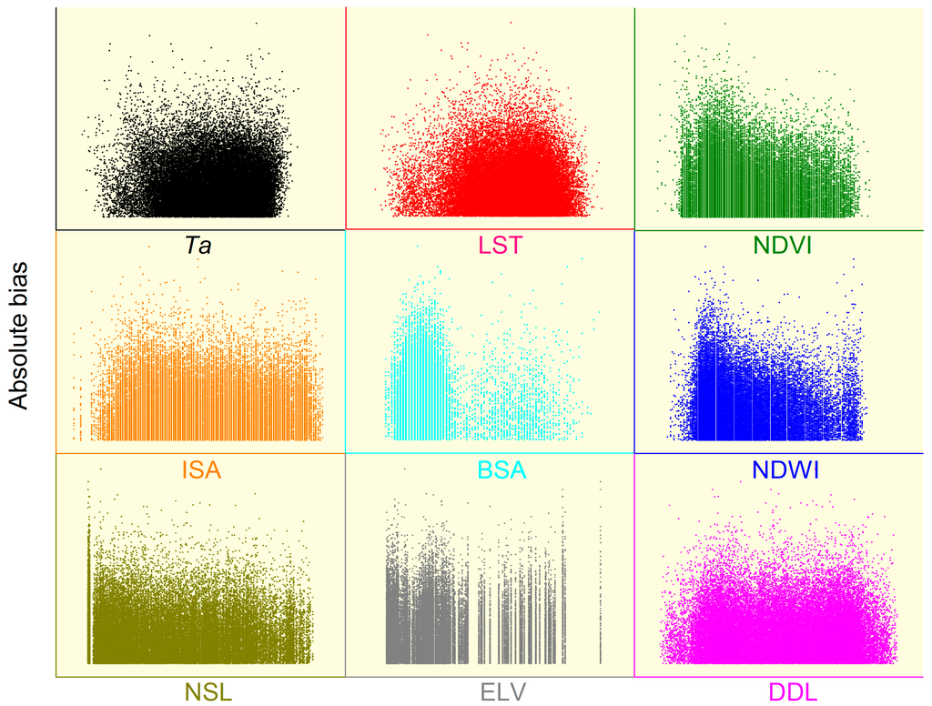
Figure 9.
Scatter plots between the absolute bias and the nine variables (i.e., Ta, LST, NDVI, ISA, BSA, NDWI, NSL, ELV, and DDL).
4.2. Temporal Patterns of Errors
Table 2 shows the statistics of RMSE and R2 by year (2.44–2.64 K and 0.97–0.98, respectively), season (2.47–2.62 K and 0.90–0.98, respectively) and month (2.40–2.63 K and 0.85–0.93, respectively). No apparent difference (<0.23 K in RMSE and 0.08 in R2) or patterns were found during years or seasons. It suggests the robustness of this model against data availability, which has shown evident seasonality in Figure 2. This was to be expected given that the time-varying coefficient modeling in the regression does not require consistently available data over time [35].

Table 2.
Error between the estimated and the measured Ta sorted by year, season, and month.
Furthermore, the trend slope, seasonal amplitude, and annual average temperature derived from the estimated Ta well agrees with those from the measured Ta (Figure 10), revealing that the inter- and intra- annual variations of Ta are well represented by this model.
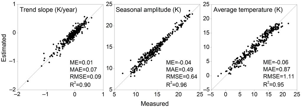
Figure 10.
Scatter plots of the trend slope, seasonal amplitude, and annual average temperature respectively, derived from the measured and the estimated Ta over the collocated weather stations.
4.3. Uncertainty Analysis
Figure 11 shows that the average uncertainty across the entire study area and period is 0.21 K, with different weather stations having uncertainties of 0.07–0.63 K and 85% of them falling in the range of 0.10–0.30 K; only three of them (i.e., less than 1%) have an uncertainty larger than 0.50 K. The largest average uncertainty was found over the forest class (0.26 K), which, however, is not greatly different in magnitude from the other classes (0.20–0.25 K, Figure 11).
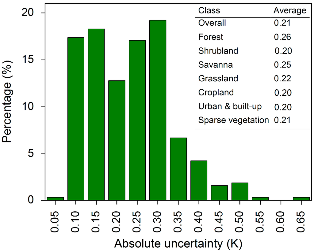
Figure 11.
Frequency of the absolute uncertainty over weather stations and the statistics of the absolute uncertainty by land cover.
4.4. Model Inter-comparison
Table 3 lists the RMSE and R2 of different empirical regressions, showing that the proposed model (i.e., composite sinusoidal coefficient regression with PC1–PC4 of the eight predictors) outperforms the other models with the lowest RMSE (2.53 K). In detail, the multi-variable regressions (models (2)–(3): RMSE = 3.33–3.35 K, R2 = 0.94–0.96) yield much improved accuracies compared to the uni-variable regression with LST (model (1): RMSE = 5.13 K, R2 = 0.89) because of the increased information added for Ta estimation; and the time-varying coefficient regressions (models (4)–(7): RMSE = 2.53–3.11 K, R2 = 0.81–0.96) are more accurate than the globally constant coefficient-scheme (models (1)–(3)). The composite sinusoidal coefficient regression directly with the eight predictors without PCA (model (5)) is unsolvable due to large amounts of unknown regression parameters. Hence, PCA is necessary from the perspectives of both variable independence and model solution. Moreover, the composite sinusoidal coefficient regression after PCA of the seven predictors excluding NSL (model (6)) presents a larger RMSE by 0.58 K than that after PCA of the eight predictors including NSL (model (7)), revealing that the use of NSL has improved the model performance. Finally, both with PC1–PC4 of the eight predictors, our proposed model using composite sinusoidal functions to describe the dynamic coefficients (model (7)) performs better than the temporally moving-window regression strategy (model (4)).

Table 3.
Averaged error of different regression models according to cross-validation.
5. Discussion
5.1. Nighttime Light, Predictor Independence, and Coefficient Dynamics
Various forms of energy use by human activities eventually turn into anthropogenic heat released into the atmosphere [44], increasing the air temperature. Considering the close relationship between NSL and urbanization [63], population [70], economy [71], energy consumption [72], etc., NSL is further found to correlate well with the anthropogenic heat flux density [44,47]. This study does not try to calculate the anthropogenic heat with NSL, but attempts to use NSL to provide relevant information on the anthropogenic heat for better Ta estimation over a large area. Results (Table 3) show that the incorporation of NSL improves the accuracy of the multi-variable linear regression (by 0.02 K in RMSE and 0.02 in R2, Table 3) and of the composite sinusoidal coefficient regression (by 0.58 K in RMSE, Table 3). With more precise spatio-temporal anthropogenic heat data or higher-resolution nighttime light data (e.g., VIIRS), the Ta estimates may be further improved.
Collinearity-induced problems [45] are well recognized in multi-variable statistical routines. Large numbers of variables accounting for different sources of influence on Ta usually mean (high) correlations among them [68,73]. Yet, previous regression-based Ta studies have not considered the collinearity among predictors an important issue primarily because the Ta estimation has mainly been conducted within the range of sampled data, i.e., when the influence of collinearity is limited [45]. This study confirms that the accuracies of linear regressions before and after PCA (with all PCs) are similar (0.02 K in difference). However, PCA is essential for the proposed method considering the increasing amount of unknown parameters with redundant datasets (Section 3.3).
Dynamic regression coefficients result in better Ta estimates than the temporally stationary coefficients (by 0.62 K or more in RMSE, Table 3) because the association of Ta and the set of predictors varies significantly by time (Figure 6). The moving window algorithm [35] is a simple and effective approach to account for this matter, while the composite sinusoidal regression we proposed yields a higher accuracy (by 0.18 K in RMSE, Table 3) probably due to the better robustness against noise and data availability (Section 4.2). It is worth noting that the coefficient functions are modeled globally, thus it is unable to capture the inter-annual change in Ta-predictor relationship.
5.2. The Seven Predictors and Complementary Predictors
Except for NSL discussed above, the seven predictors (i.e., LST, NDVI, ISA, BSA, NDWI, ELV, and DDL) selected in this study have been used in many other Ta mapping literatures due to their close correlations with Ta. Specifically, LST is the most powerful predictor because of the heat transfer between the land and the atmosphere primarily through convection [13]. NDVI and NDWI represent greenness and wetness, respectively [74], both of which strongly influence evapotranspiration and surface cooling [75], and thus a decrease in NDVI/NDWI is usually followed by a Ta rise. Similarly, ISA contributes to enhancing sensible heat flux while reducing latent heat flux [40,69] and consequently heating up the atmosphere. BSA (or albedo) indicates a reflective proportion of incoming solar radiation, and therefore a low albedo increases solar heat absorption as well as heat release to the atmosphere [13,57]. As for ELV, numerous studies have demonstrated that Ta decreases as ELV increases [68]. ELV is particularly useful for characterizing the spatial variation of Ta over a wide range of elevation.
Solar radiation is a dominant heating source for the surface, which then transfers heat to the immediate atmosphere [59]. A number of methods have been proposed to model spatio-temporal solar radiation, such as retrieval from satellite data [76], interpolation from surrounding weather stations [77,78], empirical estimation from other meteorological observations (e.g., diurnal air temperature range) [79,80], generation from weather models [81], and geometrical simulation accounting for shadows and clouds [82]. However, satellite-retrieved solar radiation has a coarse spatial resolution [76] and we lack appropriate data to calculate precise solar radiation (specifically, we lack solar radiation observations from weather stations, spatio-temporal meteorological data such as air temperature, water vapor, clouds, total optical length, and atmospheric transmittance [1], and 3D urban structures for shadow determination [82]). Alternatively, DDL was used as a substitute for daily solar radiation in calm and clear days considering their significant correlation [48], the simplicity of DDL calculation, and the spatio-temporal variance in DDL. Even though DDL is unable to reflect the effects of clouds and aerosols on the solar radiation reaching the surface, the biases can be limited because we only focused on estimating Ta under clear skies (Section 3.3).
To quantify the contributions of the seven predictors in improving the Ta estimation, we carried out statistical regressions excluding each one of the seven predictors. Results (Table 4) show that the inclusion of LST reduces RMSE by 1.59 K and increases R2 by 0.06, which illustrates the most significant role played by LST. Following it, ELV, NDWI, BSA, and DDL increase the accuracy by 0.20–0.30 K in RMSE and 0.02 in R2 (Table 4), which makes their inclusion indispensable. Also, they are readily available. On the other hand, ISA makes only a modest improvement (0.14 K in RMSE and 0.00 in R2, Table 4), which is possibly attributed to its low temporal variance (one-year resolution). Considering that the calculation of ISA is not as easy as the others, it may be removed from the predictor pool to save preprocessing time. Finally, NDVI slightly affects the predictive power (by 0.04 K in RMSE and 0.00 in R2, Table 4) and may be excluded without inducing large errors. This has been explained by the fact that NDWI, accounting for water content, has a more direct relationship to evapotranspiration and NDVI does not provide more valuable information beyond NDWI for Ta estimation [1].

Table 4.
Averaged error increase by excluding each one of the seven predictors from the regression.
Apart from the eight predictors used in this study, several additional factors are well known to impact Ta. Surface heterogeneity is one of them by affecting local surface–air interactions [83,84]. Heterogeneity can be characterized by a moving window-based semi-variogram model [85], spatial scale-based entropy spectrum [86], or landscape structure-based indices [87] and may help improve the local Ta estimation considering neighborhood interactions involved in the pixel-station pair correlation. In other words, it alters the representativeness of the station-measured observation at a pixel scale, and thus could be appropriate as a modulator to adjust the spatial distribution of the estimated Ta, as an additional weight to adjust the contributions of spatial predictors [5], or as a reference to limit the regression to the less heterogeneous areas. It should not be used as an independent variable in the regression because its relationship with Ta is not straightforward.
Sky view factor (SVF) is also known as an important predictor because it indicates the topography and building structures that affect the amount of radiation received or emitted by the ground [1]. SVF was not included in this study because we lacked fish-eye images and 3D urban structures that are commonly required for SVF calculation [88]. An alternative method was proposed by Ho et al. (2014), who used an empirically calibrated relationship of SVF with the shadow proportion derived from remote sensing images [1], which may provide an easier approach to map SVF over large areas.
5.3. Spatio-Temporal Resolutions and Extensions
First, the spatial and temporal resolutions of the eight predictors used in the regression are different, varying from 250 m to ~1 km in space and one day to one year (or multiple years) in time (Table 1). Spatially, the predictors do not have the same field of view, leading to a false collocation and correspondence. Temporally, the predictors (except for LST) have larger gaps than in situ measured daily Ta, thus incapable of characterizing intermediate Ta variations. Particularly, the yearly NSL data, the only dataset that we had access to for accounting for the anthropogenic heat impact, cannot represent intra-annual variations of anthropogenic heat discharge flux [42,89], and it consequently cannot accurately express its dynamic relationship with Ta.
Second, the spatial and temporal resolutions of the estimated Ta are the same as the finest ones of the predictors, i.e., 250 m and one day in this study. Spatially, the actual Ta can be more heterogeneous [5], especially over urban and mountainous areas (e.g., at a scale of 10–30 m [90]). Use of predictors with enhanced spatial resolutions, a spatial heterogeneity index as a modulator or weight (Section 5.2), or downscaling technologies (e.g., [90]) may help characterize local details of Ta. Temporally, Ta varies within a day, which cannot be represented by a daily average. Use of diurnally varying predictors, such as geostationary satellite-derived LST [91], is promising. Integration of the composite sinusoidal coefficient regression with a predictor-related diurnal parametric model of Ta may also be a possible solution.
Third, the proposed method can be used to generate Ta for a larger space and time domain. Spatially, the method adopts a global-window regression scheme for this study area. Nevertheless, a larger area may require not only a moving and varying regression window but also climatic and environmental factors other than surface predictors. Temporally, the method assumes periodic changes of regression coefficients. This raises a challenge of determining the breakpoint of such stationarity in time, i.e., the time domain during which the resulted empirical relationship between Ta and predictors can be applied.
5.4. Ta Estimation under Cloudy Skies
The influence of clouds on Ta estimation is three-fold. First, thick clouds induce information loss of surface predictors observed by the infrared and visible imagers on board satellites. This not only limits the spatial Ta estimation under cloudy skies [92] but also reduces the accuracy of Ta estimation under clear skies due to the decreasing amount of available data with strong seasonality [29]. Second, thin or sub-pixel clouds and cloud shadows undetected in remote sensing images degrade the pixel quality, especially for LST by presenting fairly low values. This brings in anomalies and may further distort the Ta–predictor correlations during the regression. Third, clouds influence the energy balance of the surface–air system [93,94], which is a complex process. One of the examples is the limitation of daytime warming and thus the reduction of LST–Ta lapse rate [29]. In such cases, the Ta-predictor relationship built by cloud-free data cannot handle the change in physical mechanisms under cloudy skies.
The method proposed in this study can reduce the impacts of missing or abnormal data on Ta estimation under clear skies due to the composite sinusoidal modeling of regression coefficient dynamics [29,35] (Section 4.2). However, it cannot predict Ta under cloudy skies. Kloog et al. (2014) have associated the predicted Ta under clear skies with the Ta in neighboring grid cells and then applied their relationship back to the Ta across buffers around weather stations to fill the Ta where satellite data is missing [92]. Yet, their methods have not considered the physical change in surface–air interactions. There are some studies using microwave signals (e.g., AMSR) for their advantage of penetrating clouds [95,96]. However, the resulted spatial resolution is extremely low (several to tens of kilometers). Future studies should put more effort into model development, accounting for the environmental process with cloud presence, and integrating microwave and infrared data is considered a promising solution. In addition, smog has similar effects on Ta estimation [90,97,98], which requires further focus as well.
6. Conclusions
This study proposed a method to estimate daily mean Ta based on a time-varying coefficient regression of independent components against collocated weather station Ta. The components were derived from PCA of seven commonly used predictors (i.e., LST, NDVI, ISA, BSA, NDWI, ELV, and DDL), and one never used predictor (NSL), and the regression coefficients were modeled in a dynamic fashion using composite sinusoidal functions.
The method was tested for a 12-year period over 4.32 million km2 in China. Cross-validation shows overall ME, RMSE, and R2 of −0.01 K, 2.53 K, and 0.96, respectively. Around 98% of the stations have Ta estimates within ±2.50 K limits of the observed Ta, and 60% (80%) have RMSEs smaller than 2.50 K (2.70 K). The bias of the estimated Ta shows that the method has no clear preference for air temperatures, land covers, surface properties, or nighttime light in global terms, and is robust against data availability. Moreover, the inter- and intra- annual patterns of Ta are well represented by the estimation. The average uncertainty is 0.21 K, where 85% of stations have uncertainties of 0.10–0.30 K. The model inter-comparison further reveals that the proposed method provides enhancements over six additional regressions by 0.18–2.60 K in RMSE and 0.00–0.15 in R2 because NSL was used as one of the predictors, PCA was implemented to reduce the correlations among predictors, and the regression coefficients were modeled dynamically by composite sinusoidal functions.
This method was not proposed to replace previous models, but to highlight the three remaining issues (Section 1) and to supplement the Ta mapping system. Further enhancements may consider (1) including more auxiliary data such as adding SVF as one of the predictors or using the spatial heterogeneity index as a modulator or weight to adjust the spatial distribution of Ta estimates; (2) incorporating an anthropogenic heat-related predictor with a higher spatio-temporal resolution; (3) designing a different combination of variables and selecting different amounts of principle components or using a de-collinearity process other than PCA; (4) integrating the time-varying coefficient regression with the predictor-related diurnal Ta parameters to estimate sub-daily Ta; and (5) mapping Ta in the case of clouds or smog.
Acknowledgments
This study was supported by grants from the National Natural Science Foundation of China (grants 41471348 and 41421001), the National Key Basic Research Program of China (grant 2015CB954101), the Science and Technology Program of the Institute of Geographic Sciences and Natural Resources Research, CAS (grant Y5V5001MYE), and the Fundamental Research Funds for the Central Universities (2014KJJCA16).
Author Contributions
Jinling Quan conceived, designed, and performed the experiments; Yunhao Chen analyzed the results and wrote the manuscript; Wenfeng Zhan provided constructive comments on the whole manuscript; and Zheng Guo contributed major materials and analysis tools.
Conflicts of Interest
The authors declare no conflicts of interest.
References
- Ho, H.C.; Knudby, A.; Sirovyak, P.; Xu, Y.; Hodul, M.; Henderson, S.B. Mapping maximum urban air temperature on hot summer days. Remote Sens. Environ. 2014, 154, 38–45. [Google Scholar] [CrossRef]
- Watson, R.T.; Albritton, D.L. Climate Change 2001: Synthesis Report: Third Assessment Report of the Intergovernmental Panel on Climate Change; Cambridge University Press: New York, NY, USA, 2001. [Google Scholar]
- Wang, L.; Koike, T.; Yang, K.; Yeh, P.J.F. Assessment of a distributed biosphere hydrological model against streamflow and MODIS land surface temperature in the upper tone river basin. J. Hydrol. 2009, 377, 21–34. [Google Scholar] [CrossRef]
- Garske, T.; Ferguson, N.M.; Ghani, A.C. Estimating air temperature and its influence on malaria transmission across Africa. PLoS ONE 2013, 8, e56487. [Google Scholar] [CrossRef] [PubMed]
- Nichol, J.E.; Wong, M.S. Spatial variability of air temperature and appropriate resolution for satellite-derived air temperature estimation. Int. J. Remote Sens. 2008, 29, 7213–7223. [Google Scholar] [CrossRef]
- Vancutsem, C.; Ceccato, P.; Dinku, T.; Connor, S.J. Evaluation of MODIS land surface temperature data to estimate air temperature in different ecosystems over Africa. Remote Sens. Environ. 2010, 114, 449–465. [Google Scholar] [CrossRef]
- Menzel, W.P.; Purdom, J.F.W. Introducing GOES-I: The first of a new generation of geostationary operational environmental satellites. Bull. Am. Meteorol. Soc. 1994, 75, 757–781. [Google Scholar] [CrossRef]
- Aumann, H.H.; Chahine, M.T.; Gautier, C.; Goldberg, M.D.; Kalnay, E.; McMillin, L.M.; Revercomb, H.; Rosenkranz, P.W.; Smith, W.L.; Staelin, D.H.; et al. AIRS/AMSU/HSB on the aqua mission: Design, science objectives, data products, and processing systems. IEEE Trans. Geosci. Remote Sens. 2003, 41, 253–264. [Google Scholar] [CrossRef]
- Borbas, E.E.; Seemann, S.W.; Aniko, K.; Moy, L.; Li, J.; Liam, G.; Menzel, W.P. MODIS Atmospheric Profile Retrieval Algorithm Theoretical Basis Document (collection 6); University of Wisconsin-Madison: Madison, WI, USA, 2011. [Google Scholar]
- Gao, W.; Zhao, F.; Xu, Y.; Feng, X. Validation of the surface air temperature products retrieved from the atmospheric infrared sounder over China. IEEE Trans. Geosci. Remote Sens. 2008, 46, 1783–1789. [Google Scholar]
- Sun, Y.J.; Wang, J.F.; Zhang, R.H.; Gillies, R.R.; Xue, Y.; Bo, Y.C. Air temperature retrieval from remote sensing data based on thermodynamics. Theor. Appl. Climatol. 2005, 80, 37–48. [Google Scholar] [CrossRef]
- Xu, Y.; Qin, Z.H.; Wan, H. Advances in the study of near surface air temperature retrieval from thermal infrared remote sensing. Remote Sens. Land. Resour. 2011, 9–14. [Google Scholar]
- Cristóbal, J.; Ninyerola, M.; Pons, X. Modeling air temperature through a combination of remote sensing and GIS data. J. Geophys. Res. Atmos. 2008, 113, D13106. [Google Scholar] [CrossRef]
- Florio, E.N.; Lele, S.R.; Chi Chang, Y.; Sterner, R.; Glass, G.E. Integrating AVHRR satellite data and NOAA ground observations to predict surface air temperature: A statistical approach. Int. J. Remote Sens. 2004, 25, 2979–2994. [Google Scholar] [CrossRef]
- Park, S. Integration of satellite-measured LST data into cokriging for temperature estimation on tropical and temperate islands. Int. J. Climatol. 2011, 31, 1653–1664. [Google Scholar] [CrossRef]
- Kilibarda, M.; Hengl, T.; Heuvelink, G.B.M.; Gräler, B.; Pebesma, E.; Perčec Tadić, M.; Bajat, B. Spatio-temporal interpolation of daily temperatures for global land areas at 1 km resolution. J. Geophys. Res. Atmos. 2014, 119, 2294–2313. [Google Scholar] [CrossRef]
- Chen, F.; Liu, Y.; Liu, Q.; Qin, F. A statistical method based on remote sensing for the estimation of air temperature in China. Int. J. Climatol. 2015, 35, 2131–2143. [Google Scholar] [CrossRef]
- Lennon, J.J.; Turner, J.R.G. Predicting the spatial distribution of climate: Temperature in great Britain. J. Anim. Ecol. 1995, 64, 370–392. [Google Scholar] [CrossRef]
- Stahl, K.; Moore, R.D.; Floyer, J.A.; Asplin, M.G.; McKendry, I.G. Comparison of approaches for spatial interpolation of daily air temperature in a large region with complex topography and highly variable station density. Agric. For. Meteorol. 2006, 139, 224–236. [Google Scholar] [CrossRef]
- Sun, H.; Chen, Y.; Gong, A.; Zhao, X.; Zhan, W.; Wang, M. Estimating mean air temperature using MODIS day and night land surface temperatures. Theor. Appl. Climatol. 2014, 118, 81–92. [Google Scholar] [CrossRef]
- Sandholt, I.; Rasmussen, K.; Andersen, J. A simple interpretation of the surface temperature/vegetation index space for assessment of surface moisture status. Remote Sens. Environ. 2002, 79, 213–224. [Google Scholar] [CrossRef]
- Stisen, S.; Sandholt, I.; Nørgaard, A.; Fensholt, R.; Eklundh, L. Estimation of diurnal air temperature using MSG SEVIRI data in West Africa. Remote Sens. Environ. 2007, 110, 262–274. [Google Scholar] [CrossRef]
- Xu, Y.; Qin, Z.; Shen, Y. Study on the estimation of near-surface air temperature from MODIS data by statistical methods. Int. J. Remote Sens. 2012, 33, 7629–7643. [Google Scholar] [CrossRef]
- Kloog, I.; Chudnovsky, A.; Koutrakis, P.; Schwartz, J. Temporal and spatial assessments of minimum air temperature using satellite surface temperature measurements in Massachusetts, USA. Sci. Total Environ. 2012, 432, 85–92. [Google Scholar] [CrossRef] [PubMed]
- Blennow, K. Modelling minimum air temperature in partially and clear felled forests. Agric. For. Meteorol. 1998, 91, 223–235. [Google Scholar] [CrossRef]
- Emamifar, S.; Rahimikhoob, A.; Noroozi, A.A. Daily mean air temperature estimation from MODIS land surface temperature products based on M5 model tree. Int. J. Climatol. 2013, 33, 3174–3181. [Google Scholar] [CrossRef]
- Shen, S.; Leptoukh, G.G. Estimation of surface air temperature over central and eastern Eurasia from MODIS land surface temperature. Environ. Res. Lett. 2011, 6, 045206. [Google Scholar] [CrossRef]
- Jang, J.D.; Viau, A.A.; Anctil, F. Neural network estimation of air temperatures from AVHRR data. Int. J. Remote Sens. 2004, 25, 4541–4554. [Google Scholar] [CrossRef]
- Benali, A.; Carvalho, A.C.; Nunes, J.P.; Carvalhais, N.; Santos, A. Estimating air surface temperature in Portugal using MODIS LST data. Remote Sens. Environ. 2012, 124, 108–121. [Google Scholar] [CrossRef]
- Fu, G.; Shen, Z.; Zhang, X.; Shi, P.; Zhang, Y.; Wu, J. Estimating air temperature of an alpine meadow on the northern Tibetan Plateau using MODIS land surface temperature. Acta Ecol. Sinica 2011, 31, 8–13. [Google Scholar] [CrossRef]
- Vogt, J.V.; Viau, A.A.; Paquet, F. Mapping regional air temperature fields using satellite-derived surface skin temperatures. Int. J. Climatol. 1997, 17, 1559–1579. [Google Scholar] [CrossRef]
- Muller, C.L.; Chapman, L.; Grimmond, C.S.B.; Young, D.T.; Cai, X. Sensors and the city: A review of urban meteorological networks. Int. J. Climatol. 2013, 33, 1585–1600. [Google Scholar] [CrossRef]
- Muller, C.L.; Chapman, L.; Grimmond, C.S.B.; Young, D.T.; Cai, X.-M. Toward a standardized metadata protocol for urban meteorological networks. Bull. Am. Meteorol. Soc. 2013, 94, 1161–1185. [Google Scholar] [CrossRef]
- Shao, Q.; Sun, C.; Liu, J.; He, J.; Kuang, W.; Tao, F. Impact of urban expansion on meteorological observation data and overestimation to regional air temperature in China. J. Geogr. Sci. 2011, 21, 994–1006. [Google Scholar] [CrossRef]
- Good, E. Daily minimum and maximum surface air temperatures from geostationary satellite data. J. Geophys. Res. Atmos. 2015, 120, 2306–2324. [Google Scholar] [CrossRef]
- Nichol, J.E.; To, P.H. Temporal characteristics of thermal satellite images for urban heat stress and heat island mapping. ISPRS J. Photogramm. Remote Sens. 2012, 74, 153–162. [Google Scholar] [CrossRef]
- Sailor, D.J.; Lu, L. A top down methodology for developing diurnal and seasonal anthropogenic heating profiles for urban areas. Atmos. Environ. 2004, 38, 2737–2748. [Google Scholar] [CrossRef]
- Fan, H.; Sailor, D.J. Modeling the impacts of anthropogenic heating on the urban climate of Philadelphia: A comparison of implementations in two PBL schemes. Atmos. Environ. 2005, 39, 73–84. [Google Scholar] [CrossRef]
- Salamanca, F.; Georgescu, M.; Mahalov, A.; Moustaoui, M.; Wang, M. Anthropogenic heating of the urban environment due to air conditioning. J. Geophys. Res. Atmos. 2014, 119, 5949–5965. [Google Scholar] [CrossRef]
- Oke, T.R. The urban energy balance. Progr. Phys. Geogr. 1988, 12, 471–508. [Google Scholar] [CrossRef]
- Taha, H.; Akbari, H.; Sailor, D.; Ritschard, R. Causes and Effects of Heat Islands: Sensitivity to Surface Parameters and Anthropogenic Heating; Lawrence Berkeley Lab: Berkeley, CA, USA, 1992.
- Sailor, D.J.; Georgescu, M.; Milne, J.M.; Hart, M.A. Development of a national anthropogenic heating database with an extrapolation for international cities. Atmos. Environ. 2015, 118, 7–18. [Google Scholar] [CrossRef]
- Kato, S.; Yamaguchi, Y. Analysis of urban heat-island effect using ASTER and ETM+ data: Separation of anthropogenic heat discharge and natural heat radiation from sensible heat flux. Remote Sens. Environ. 2005, 99, 44–54. [Google Scholar] [CrossRef]
- Chen, B.; Shi, G.; Wang, B.; Zhao, J.; Tan, S. Estimation of the anthropogenic heat release distribution in China from 1992 to 2009. Acta Meteorol. Sinica 2012, 26, 507–515. [Google Scholar] [CrossRef]
- Dormann, C.F.; Elith, J.; Bacher, S.; Buchmann, C.; Carl, G.; Carré, G.; Marquéz, J.R.G.; Gruber, B.; Lafourcade, B.; Leitão, P.J.; et al. Collinearity: A review of methods to deal with it and a simulation study evaluating their performance. Ecography 2013, 36, 27–46. [Google Scholar] [CrossRef]
- Lee, J.S. The Geology of China; Thomas Murky & Co.: London, UK, 1939; p. 31. [Google Scholar]
- Zhou, D.C.; Zhao, S.Q.; Liu, S.G.; Zhang, L.X.; Zhu, C. Surface urban heat island in China's 32 major cities: Spatial patterns and drivers. Remote Sens. Environ. 2014, 152, 51–61. [Google Scholar] [CrossRef]
- Angstrom, A. Solar and terrestrial radiation. Report to the international commission for solar research on actinometric investigations of solar and atmospheric radiation. Q. J. R. Meteorol. Soc. 1924, 50, 121–126. [Google Scholar] [CrossRef]
- Wan, Z.M.; Dozier, J. A generalized split-window algorithm for retrieving land-surface temperature from space. IEEE Trans. Geosci. Remote Sens. 1996, 34, 892–905. [Google Scholar]
- Wan, Z.M. New refinements and validation of the collection-6 MODIS land-surface temperature/emissivity product. Remote Sens. Environ. 2014, 140, 36–45. [Google Scholar] [CrossRef]
- Hulley, G.C.; Hughes, C.G.; Hook, S.J. Quantifying uncertainties in land surface temperature and emissivity retrievals from aster and MODIS thermal infrared data. J. Geophys. Res. 2012, 117, D23113. [Google Scholar] [CrossRef]
- Wan, Z.M. New refinements and validation of the MODIS land-surface temperature/emissivity products. Remote Sens. Environ. 2008, 112, 59–74. [Google Scholar] [CrossRef]
- Neteler, M. Estimating daily land surface temperatures in mountainous environments by reconstructed MODIS LST data. Remote Sens. 2010, 2, 333–351. [Google Scholar] [CrossRef]
- Wang, K.; Liang, S. Evaluation of aster and MODIS land surface temperature and emissivity products using long-term surface longwave radiation observations at SURFRAD sites. Remote Sens. Environ. 2009, 113, 1556–1565. [Google Scholar] [CrossRef]
- Wang, W.; Liang, S.; Meyers, T. Validating MODIS land surface temperature products using long-term nighttime ground measurements. Remote Sens. Environ. 2008, 112, 623–635. [Google Scholar] [CrossRef]
- Lagouarde, J.P.; Hénon, A.; Irvine, M.; Voogt, J.; Pigeon, G.; Moreau, P.; Masson, V.; Mestayer, P. Experimental characterization and modelling of the nighttime directional anisotropy of thermal infrared measurements over an urban area: Case study of Toulouse (France). Remote Sens. Environ. 2012, 117, 19–33. [Google Scholar] [CrossRef]
- Quan, J.L.; Chen, Y.H.; Zhan, W.F.; Wang, J.F.; Voogt, J.; Wang, M.J. Multi-temporal trajectory of the urban heat island centroid in Beijing, China based on a Gaussian volume model. Remote Sens. Environ. 2014, 149, 33–46. [Google Scholar] [CrossRef]
- Yang, F.; Matsushita, B.; Fukushima, T.; Yang, W. Temporal mixture analysis for estimating impervious surface area from multi-temporal MODIS NDVI data in Japan. ISPRS J. Photogramm. Remote Sens. 2012, 72, 90–98. [Google Scholar] [CrossRef]
- Abraha, M.G.; Savage, M.J. Comparison of estimates of daily solar radiation from air temperature range for application in crop simulations. Agric. For. Meteorol. 2008, 148, 401–416. [Google Scholar] [CrossRef]
- Gao, B.C. NDWI A normalized difference water index for remote sensing of vegetation liquid water from space. Remote Sens. Environ. 1996, 58, 257–266. [Google Scholar] [CrossRef]
- Liu, Z.; He, C.; Zhang, Q.; Huang, Q.; Yang, Y. Extracting the dynamics of urban expansion in China using DMSP-OLS nighttime light data from 1992 to 2008. Landsc. Urban Plan. 2012, 106, 62–72. [Google Scholar] [CrossRef]
- Elvidge, C.D.; Ziskin, D.; Baugh, K.E.; Tuttle, B.T.; Ghosh, T.; Pack, D.W.; Erwin, E.H.; Zhizhin, M. A fifteen year record of global natural gas flaring derived from satellite data. Energies 2009, 2, 595–622. [Google Scholar] [CrossRef]
- Ma, T.; Zhou, Y.; Zhou, C.; Haynie, S.; Pei, T.; Xu, T. Night-time light derived estimation of spatio-temporal characteristics of urbanization dynamics using DMSP/OLS satellite data. Remote Sens. Environ. 2015, 158, 453–464. [Google Scholar] [CrossRef]
- Göttsche, F.M.; Olesen, F.S. Modelling of diurnal cycles of brightness temperature extracted from Meteosat data. Remote Sens. Environ. 2001, 76, 337–348. [Google Scholar] [CrossRef]
- Rajagopalan, B.; Lall, U. A k-nearest-neighbor simulator for daily precipitation and other weather variables. Water Resour. Res. 1999, 10, 3089–3101. [Google Scholar] [CrossRef]
- Singh, A.; Harrison, A. Standardized principal components. Int. J. Remote Sens. 1985, 6, 883–896. [Google Scholar] [CrossRef]
- Jain, A.; Nandakumar, K.; Ross, A. Score normalization in multimodal biometric systems. Pattern Recognit. 2005, 38, 2270–2285. [Google Scholar] [CrossRef]
- Zakšek, K.; Oštir, K. Downscaling land surface temperature for urban heat island diurnal cycle analysis. Remote Sens. Environ. 2012, 117, 114–124. [Google Scholar] [CrossRef]
- Quan, J.L.; Zhan, W.F.; Chen, Y.H.; Wang, M.; Wang, J.F. Time series decomposition of remotely sensed land surface temperature and investigation of trends and seasonal variations in surface urban heat islands. J. Geophys. Res. Atmos. 2016, 121, 2638–2657. [Google Scholar] [CrossRef]
- Amaral, S.; Monteiro, A.M.V.; Camara, G.; Quintanilha, J.A. DMSP/OLS nighttime light imagery for urban population estimates in the Brazilian Amazon. Int. J. Remote Sens. 2006, 27, 855–870. [Google Scholar] [CrossRef]
- Ghosh, T.; Anderson, S.; Powell, L.R.; Sutton, C.P.; Elvidge, D.C. Estimation of Mexico's informal economy and remittances using nighttime imagery. Remote Sens. 2009, 1, 418–444. [Google Scholar] [CrossRef]
- Letu, H.; Hara, M.; Yagi, H.; Naoki, K.; Tana, G.; Nishio, F.; Shuhei, O. Estimating energy consumption from night-time DMPS/OLS imagery after correcting for saturation effects. Int. J. Remote Sens. 2010, 31, 4443–4458. [Google Scholar] [CrossRef]
- Bechtel, B.; Zakšek, K.; Hoshyaripour, G. Downscaling land surface temperature in an urban area: A case study for Hamburg, Germany. Remote Sens. 2012, 4, 3184–3200. [Google Scholar] [CrossRef]
- Gu, Y.; Hunt, E.; Wardlow, B.; Basara, J.B.; Brown, J.F.; Verdin, J.P. Evaluation of MODIS NDVI and NDWI for vegetation drought monitoring using Oklahoma Mesonet soil moisture data. Geophys. Res. Lett. 2008, 35, L22401. [Google Scholar] [CrossRef]
- Rizwan, A.M.; Dennis, L.Y.C.; Liu, C. A review on the generation, determination and mitigation of urban heat island. J. Environ. Sci. 2008, 20, 120–128. [Google Scholar] [CrossRef]
- Janjai, S.; Pankaew, P.; Laksanaboonsong, J.; Kitichantaropas, P. Estimation of solar radiation over cambodia from long-term satellite data. Renew. Energy 2011, 36, 1214–1220. [Google Scholar] [CrossRef]
- Reddy, K.S.; Ranjan, M. Solar resource estimation using artificial neural networks and comparison with other correlation models. Energy Conv. Manag. 2003, 44, 2519–2530. [Google Scholar] [CrossRef]
- Soltani, A.; Meinke, H.; de Voil, P. Assessing linear interpolation to generate daily radiation and temperature data for use in crop simulations. Eur. J. Agron. 2004, 21, 133–148. [Google Scholar] [CrossRef]
- Bristow, K.L.; Campbell, G.S. On the relationship between incoming solar radiation and daily maximum and minimum temperature. Agric. For. Meteorol. 1984, 31, 159–166. [Google Scholar] [CrossRef]
- Mahmood, R.; Hubbard, K.G. Effect of time of temperature observation and estimation of daily solar radiation for the Northern Great Plains, USA. Agron. J. 2002, 94, 723–733. [Google Scholar] [CrossRef]
- Hansen, J.W. Stochastic daily solar irradiance for biological modeling applications. Agric. For. Meteorol. 1999, 94, 53–63. [Google Scholar] [CrossRef]
- Zakšek, K.; Podobnikar, T.; Oštir, K. Solar radiation modelling. Comput. Geosci. 2005, 31, 233–240. [Google Scholar] [CrossRef]
- Avissar, R.; Pielke, R.A. A parameterization of heterogeneous land surfaces for atmospheric numerical models and its impact on regional meteorology. Mon. Weather Rev. 1989, 117, 2113–2136. [Google Scholar] [CrossRef]
- Huang, H.-Y.; Margulis, S.A. On the impact of surface heterogeneity on a realistic convective boundary layer. Water Resour. Res. 2009, 45, W04425. [Google Scholar] [CrossRef]
- Garrigues, S.; Allard, D.; Baret, F.; Weiss, M. Quantifying spatial heterogeneity at the landscape scale using variogram models. Remote Sens. Environ. 2006, 103, 81–96. [Google Scholar] [CrossRef]
- Hintz, M.; Lennartz-Sassinek, S.; Liu, S.; Shao, Y. Quantification of land surface heterogeneity via entropy spectrum method. J. Geophys. Res. Atmos. 2014, 119, 8764–8777. [Google Scholar] [CrossRef]
- Chen, Y.H.; Shi, P.J.; Li, X.B. Research on spatial thermal environment in Shanghai city based on remote sensing and GIS. Acta Geod. Cartogr. Sinica 2002, 31, 139–144. [Google Scholar]
- Unger, J. Intra-urban relationship between surface geometry and urban heat island: Review and new approach. Clim. Res. 2004, 27, 253–264. [Google Scholar] [CrossRef]
- Hu, D.; Yang, L.M.; Zhou, J.; Deng, L. Estimation of urban energy heat flux and anthropogenic heat discharge using ASTER image and meteorological data: Case study in Beijing metropolitan area. J. Appl. Remote Sens. 2012, 6, 063559. [Google Scholar] [CrossRef]
- Holden, Z.A.; Abatzoglou, J.T.; Luce, C.H.; Baggett, S.L. Empirical downscaling of daily minimum air temperature at very fine resolutions in complex terrain. Agric. For. Meteorol. 2011, 151, 1066–1073. [Google Scholar] [CrossRef]
- Bechtel, B.; Wiesner, S.; Zakšek, K. Estimation of dense time series of urban air temperatures from multitemporal geostationary satellite data. IEEE J. Sel. Top. Appl. Earth Obs. Remote Sens. 2014, 7, 4129–4137. [Google Scholar] [CrossRef]
- Kloog, I.; Nordio, F.; Coull, B.A.; Schwartz, J. Predicting spatiotemporal mean air temperature using MODIS satellite surface temperature measurements across the northeastern USA. Remote Sens. Environ. 2014, 150, 132–139. [Google Scholar] [CrossRef]
- Jin, M.; Dickinson, R.E. Land surface skin temperature climatology: Benefitting from the strengths of satellite observations. Environ. Res. Lett. 2010, 5, 044004. [Google Scholar] [CrossRef]
- Pepin, N.C.; Norris, J.R. An examination of the differences between surface and free-air temperature trend at high-elevation sites: Relationships with cloud cover, snow cover, and wind. J. Geophys. Res. Atmos. 2005, 110, D24112. [Google Scholar] [CrossRef]
- Jang, K.; Kang, S.; Kimball, S.J.; Hong, Y.S. Retrievals of all-weather daily air temperature using MODIS and AMSR-E data. Remote Sens. 2014, 6, 8387–8404. [Google Scholar] [CrossRef]
- Jones, L.A.; Ferguson, C.R.; Kimball, J.S.; Zhang, K.; Chan, S.T.K.; McDonald, K.C.; Njoku, E.G.; Wood, E.F. Satellite microwave remote sensing of daily land surface air temperature minima and maxima from amsr-e. IEEE J. Sel. Top. Appl. Earth Obs. Remote Sens. 2010, 3, 111–123. [Google Scholar] [CrossRef]
- Köhn, J.; Royer, A. Microwave brightness temperature as an indicator of near-surface air temperature over snow in Canadian northern regions. Int. J. Remote Sens. 2012, 33, 1126–1138. [Google Scholar] [CrossRef]
- Zhan, W.; Zhou, J.; Ju, W.; Li, M.; Sandholt, I.; Voogt, J.; Yu, C. Remotely sensed soil temperatures beneath snow-free skin-surface using thermal observations from tandem polar-orbiting satellites: An analytical three-time-scale model. Remote Sens. Environ. 2014, 143, 1–14. [Google Scholar] [CrossRef]
© 2016 by the authors; licensee MDPI, Basel, Switzerland. This article is an open access article distributed under the terms and conditions of the Creative Commons Attribution (CC-BY) license (http://creativecommons.org/licenses/by/4.0/).

