1. Introduction
The Arctic has emerged as an important focal point for the study of climate change, with rates of recent climate warming approximately twice the global average [
1]. Climate warming is projected to continue in this region with broad implications for sensitive tundra ecosystems and globally important climate feedbacks [
2]. Observations also suggest that permafrost thaw is common in high-latitude ecosystems and is expected to drive changes in climate forcing through biogeochemical and biophysical feedbacks [
3]. These interacting feedbacks will take place in an environment expected to undergo dramatic geomorphic change and landscape reorganization [
4]. Increases in active-layer thickness at some locations have driven ecosystem responses, including changes in vegetation cover [
5]. Changes in vegetation community composition and distribution can affect albedo and energy partitioning in the Arctic [
5,
6]. Furthermore, recent studies indicate that the phenology of vegetation (the timing of processes throughout the growing season) is a primary indicator of the dynamic responses of terrestrial ecosystems to climate change [
7].
Terrestrial vegetation plays an important role in the dynamics of the Earth system through water and energy exchange and is one of the largest sources of uncertainty in climate change predictions [
8]. In the Accelerated Climate Model for Energy (ACME) land model (ALM), as with most other models [
8], vegetation is not represented as biomes, but rather as plant functional types (PFTs) [
9]. Each PFT groups plant species that share similar responses to environmental factors and effects on ecosystems [
10,
11]. Most climate models currently use only two PFTs (one grass and one shrub type) to represent Arctic vegetation, greatly limiting the representation of plant functions and feedbacks in simulating Arctic responses to a warming climate [
9]. Chapin et al. [
12,
13] recommended the use of Arctic- and boreal-specific PFTs in vegetation models, including deciduous shrubs, evergreen shrubs, sedges, grasses, forbs,
Sphagnum moss, non-
Sphagnum moss and lichens, to capture Arctic vegetation processes.
Poulter et al. [
14] showed that accurate PFT datasets are important for reducing the uncertainty of terrestrial biogeochemical processes to climate variability in Earth system models. Satellite datasets have been used to extract PFT information from the landscape and can contribute to improved predictive capabilities of land-atmosphere interactions [
15]. Different remote sensing-based PFT products are available for Earth system models [
11,
14,
16]. However, these products for parameterizing PFTs are at a coarse resolution (hundreds of meters to kilometers). New high resolution products are needed to capture the fine-scale heterogeneity of PFTs observed in the field.
There is a growing interest in understanding and resolving the subgrid scale processes in heterogeneous Arctic ecosystem. The U.S. Department of Energy’s Office of Science Next Generation Ecosystem Experiments (NGEE) Arctic project seeks to couple high-resolution models to Earth system models to represent Arctic land surface and subsurface processes and their interactions in a warming climate, such as high-resolution hydrologic (e.g., Arctic Terrestrial Simulator, PFLOTRAN) [
17,
18], biogeochemical (PFLOTRAN) [
19] and biosphere models (CLM-PFLOTRAN) [
19], can run at fine spatial and temporal resolutions and require high-resolution datasets. This need for parameterizing high-resolution land surface models require new approaches for developing such high-resolution products.
Most optical remote sensing studies of Arctic vegetation consist of coarse resolution datasets from 30 m–250 m [
15,
20,
21], and few studies have been performed at the WorldView-2 resolution (∼0.5–∼2 m) [
22]. Medium resolution satellite datasets are useful for characterizing PFT coverage at regional to global scales, but there are challenges to integrating such datasets with sparse small-scale point measurements for upscaling. WorldView-2 multispectral satellite imagery has a much higher spatial resolution and can help capture the fine-scale variation in PFTs.
There has been considerable recent progress in the development of methods for handling and analyzing high-resolution remote sensing data. Dalmayne et al. [
23] used WorldView-2 satellite spectral dissimilarity to infer environmental heterogeneity in dry semi-natural grasslands, which revealed a significant positive association between spectral dissimilarity and fine-scale plant species beta diversity. Ramoelo et al. [
24] monitored leaf N and above-ground biomass as an indicator of rangeland quality and quantity using WorldView-2 satellite images and the random forest technique. Karna et al. [
25] integrated WorldView-2 satellite images with small footprint airborne LiDAR data for estimation of tree carbon at the species level. Mutanga et al. [
26] demonstrated the utility of WorldView-2 imagery and random forest regression in estimating and mapping vegetation biomass at high density. Gangodagamage et al. [
27] used LiDAR and WorldView-2 data to show variability in active layer thickness and the controls of local microtopography in Barrow, AK. These studies suggest that high spatial resolution data, such as WorldView-2 and LiDAR data, may potentially contribute to the development of improved methods for the mapping and monitoring of vegetation at fine scales and use for high-resolution land surface models.
Phenology, seasonal changes in plants from year to year, can be a useful proxy for monitoring vegetation [
28]. Remote sensing phenology studies use data gathered by satellite sensors that measure wavelengths of light absorbed and reflected by green plants. Several remote sensing studies of phenology use satellites to track seasonal changes in vegetation on regional, continental and global scales [
29,
30]. However, very few studies have used high-resolution (e.g., WorldView-2/3) image time series for understanding seasonal patterns in reflectance that can enable the detection and change of vegetation at fine spatial scales. It is important to develop analysis techniques to capitalize on rich time series of imagery from high-resolution sensors as they become more available. In this study, we hypothesize that capturing the vegetation phenology using repeat imagery from high-resolution satellite data will help improve the characterization of the PFT distributions at our study site.
In situ field measurements are made at relatively few and specific geographic points and are representative samples of regions of similar characteristics. To upscale the in situ field measurements at larger scales for estimating landscape-scale characteristics, the representativeness of those measurements must be quantified. A representativeness metric provides insight into coverage provides by the field samples, the selection of optimal sampling locations and offer a quantitative approach for down-scaling of remote sensing data and extrapolation of measurements to unsampled domains [
31]. Sampling in under-represented sites, guided by the representativeness metric, can lead to improved accuracy in the upscaling of the measured quantity (PFTs in current study).
The objectives of this study are to: (1) characterize the landscape using high-resolution multi-spectral WorldView-2 satellite imagery and LiDAR-derived DEM; (2) use an interpolation algorithm for upscaling vegetation surveys and creating gridded PFT datasets based on remote sensing imagery; (3) use salient differences in growing season phenology (timing and magnitude of greenness) to help discriminate among various PFTs; (4) quantify the uncertainty in gridded estimates of PFT distributions upscaled from point observations using a representativeness metric; (5) devise optimal sampling strategies for ground-truthing and to improve PFT estimates and reduce uncertainty.
Interpolation is a process of using measurements about a process at a limited number of point locations to make estimates about the process at other, unmeasured locations. In this study, the term upscaling is defined as an interpolation process to employ point measurements to develop gridded estimates. An important objective was to develop a new data analytic approach to mine high resolution spectral remote sensing datasets for signatures of surface vegetation to develop estimates of PFT distributions at high spatial resolution (0.25 m × 0.25 m) across a fragmented Arctic landscape.
2. Methodology
The Methodology section follows the structure shown in
Figure 1.
Section 2.1 describes the study sites (
Section 2.1.1), field vegetation surveys (
Section 2.1.2) and the remote sensing datasets used in this study (
Section 2.1.3). The
k-means algorithm for stratifying the heterogeneous landscape using remote sensing datasets is described in
Section 2.2.
Section 2.3 describes the methodology to quantify the representativeness of the field vegetation surveys in the context of the larger study region.
Section 2.4 presents the approach for statistically upscaling the PFT distribution on the landscape using the clusters from
Section 2.2.
Section 2.5 describes the approach for the validation of the upscaled PFT distributions using a bootstrapping approach (
Section 2.5.1) and on the ground via additional field surveys (
Section 2.5.2).
2.1. Study Area and Datasets
2.1.1. Study Area
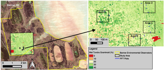
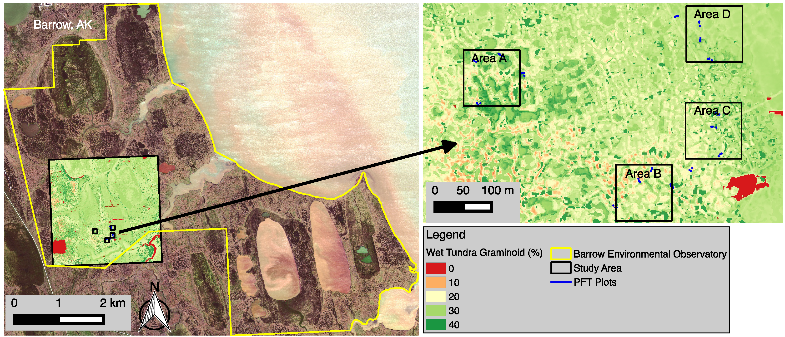
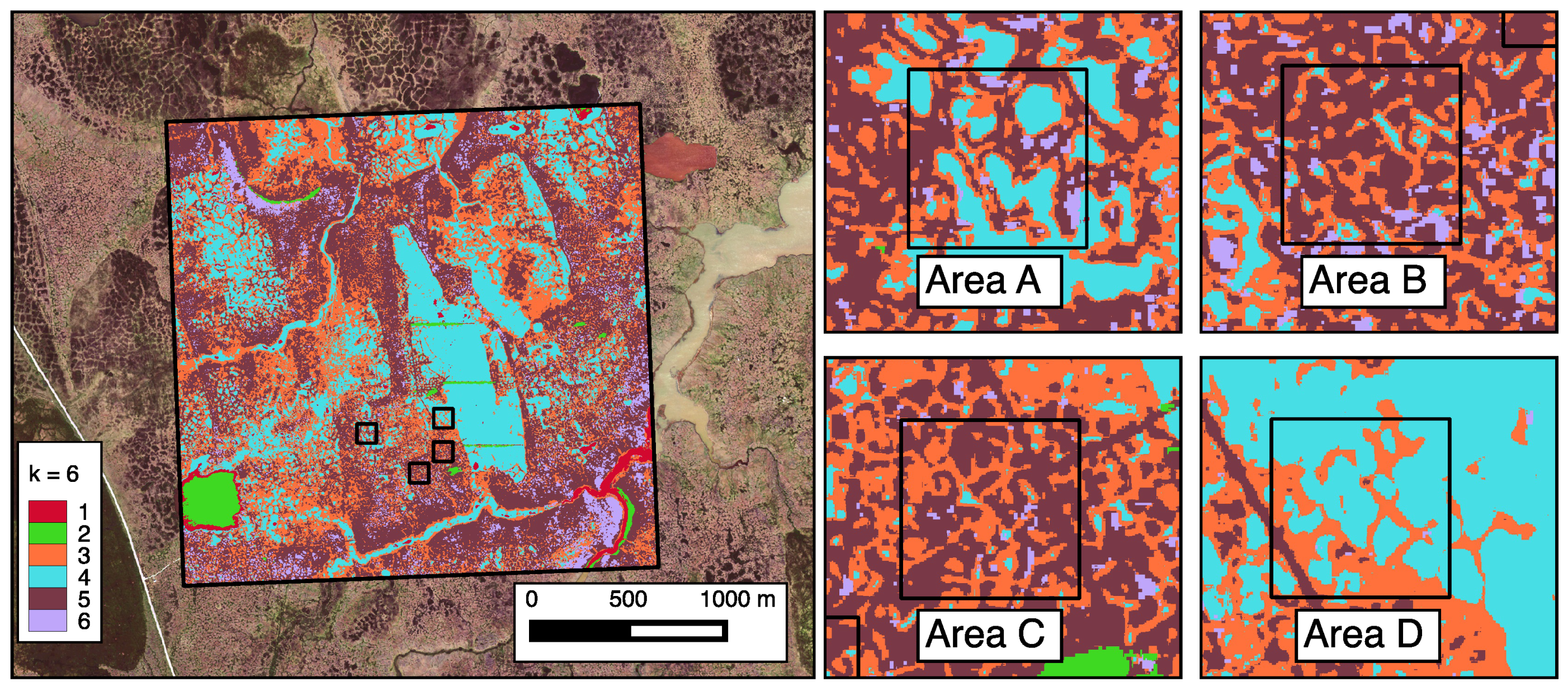
The study area is located within the Barrow Environmental Observatory (BEO) located 6 km east of Barrow, Alaska (71.3°N, 156.5°W), as part of the U.S. Department of Energy’s Office of Science Next Generation Ecosystem Experiments (NGEE) Arctic project (
Figure 2). The NGEE Arctic project seeks to reduce uncertainty in climate prediction by better understanding critical land–atmosphere feedbacks in terrestrial ecosystems of Alaska. NGEE Arctic has established four 100 m × 100 m intensively-sampled areas (
Figure 2A–D;
Table 1) within the BEO. The mean annual air temperature is −12 °C, and the mean temperature from June–August is 3.2 °C [
32]. The annual adjusted precipitation is 173 mm·year
[
32], with the majority of precipitation falling during the summer months. Soils on the BEO are generally classified as Gelisols, which are characterized by an organic-rich surface layer underlain by a horizon of silty clay to silt-loam textured mineral material and a frozen organic-rich mineral layer. The seasonally-active-layer thickness ranges between 30 and 90 cm at the BEO [
33,
34].
The BEO is a low relief landscape, with <7-m differences in topography (
Figure 2) and a low hydraulic gradient region characterized by thaw lakes and drained basins [
35]. Seasonal freeze and thaw processes have produced a polygonal network of high centered polygons, low centered polygons and transitional polygons [
36].
Table 1 lists the polygonal characteristics for Areas A–D.
2.1.2. Field Vegetation Surveys
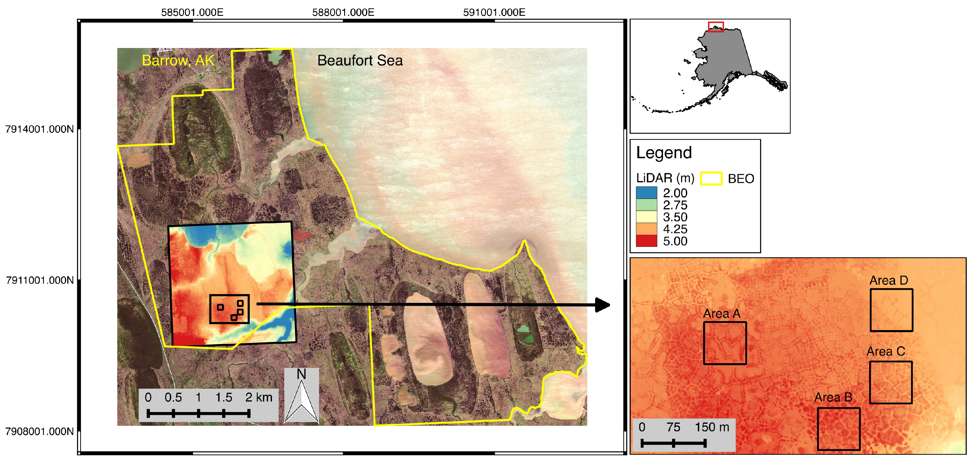
Plant community surveys were undertaken at 48 permanently marked 1 m × 1 m plots in and around the four NGEE Arctic sites (12 plots for Areas A, B, C and D) dominated by differing polygon types (
Table 1;
Figure 2). Plots were located in homogeneous vegetation communities in the centers, edges and troughs of four polygons per area and the locations of the plot corners surveyed using dGPS. Aerial fractional coverages of all vascular, bryophyte and lichen species or genera and bare ground were visually estimated by a single surveyor between 17 July and 29 July 2012. Rare species were assigned nominal values of 0.1% (single individual), 1% (multiple individuals) and 3% (few individuals forming <5% coverage) and all remaining species recorded to the nearest 5%. Canopies were considered to have two layers, with taller vascular plant coverage of up to 100% and a ground layer including some or all of mosses, lichens, prostrate vascular plants and bare ground with coverage of up to 100%. Standing water was not present in any plots at the time of the survey, although in polygon troughs, moss and sedge vegetation was “floating” on saturated soil. Recorded species were assigned to PFTs using the descriptions of Chapin et al. [
13], with the “grass” category modified here to “wet tundra graminoids” (to include true grasses, such as
Dupontia fisheri) and the “sedge” category to “dry tundra graminoids” (to include
Luzula spp.). Fractional coverage of any PFT was the sum of all species in that category. Shrubs (deciduous and evergreen) were a very small component (mean of 1.27% for Areas A, B, C and D) of the plant community composition across the study region and were thus omitted in this analysis.
2.1.3. Remote Sensing Datasets
We used cloud-free WorldView-2 satellite (DigitalGlobe) multispectral imagery (∼2 m resolution) provided by the Polar Geospatial Center (PGC). The imagery was radiometrically corrected by DigitalGlobe and orthorectified by the PGC. We assume the geolocational error to be minimal, but some errors may be possible. We analyzed the blue (450–510 nm), green (510–581 nm), red (630–690 nm) and near-infrared (NIR) (770–895 nm) bands. Images from 6 different days during the 2010 growing season (10 June, 24 June, 21 July, 26 July, 3 August and 4 August) were acquired to capture the vegetation phenology.
The 0.25-m spatial resolution LiDAR digital elevation model (DEM) used in this study was developed by AeroMetric, now known as Quantum Spatial, Inc., and flown on 4 October 2005. The DEM pixel values represent the ground elevation above sea level, with elevation values ranging from 0.00–7.06 m (mean 3.82 m). The DEM pixels show a mean difference of 0.003 meters (median = 0.004,
= 0.043 m) compared to survey data (
n = 286 points) collected in August 2006. More information on the LiDAR dataset can be found at
http://dx.doi.org/10.5065/D6KS6PQ3. We assumed that the spatial variability of PFTs during WorldView-2 and LiDAR image collection in 2010 and 2005, respectively, was similar to the field surveys conducted during 2012 for the comparison of remotely-sensed data with field observations.
We converted all WorldView-2 imagery to top-of-atmosphere (TOA) reflectance. TOA reflectance is the reflectance measured by the space-based sensor flying higher than the Earth’s atmosphere. TOA reflectance does not account for topographic, atmospheric or bidirectional reflectance distribution function (BRDF) differences. The pixel digital numbers (DNs) were converted to top-of-atmosphere band-averaged reflectance according to Updike and Comp [
37].
A commonly-used index for the estimation of vegetation properties using satellite remote sensing is the normalized difference vegetation index (NDVI). NDVI is based on the contrast between absorption in the red band by chlorophyll pigments and reflectance in the NIR band caused by internal scattering within leaves [
38]. NDVI calculated from different WorldView-2 satellite bands has been used for the estimation of fine-scale species diversity in semi-natural grasslands [
23]. NDVI was calculated as:
where
and
stand for the TOA reflectance measurements acquired in the red and NIR regions, respectively. TOA reflectance values vary between 0.0 and 1.0; thus, NDVI varies between
(no vegetation) and
(green vegetation).
The WorldView-2 datasets were resampled to the LiDAR resolution of 0.25 m × 0.25 m, using the nearest-neighbor resampling algorithm. The spectral and topographic characteristics were extracted from the remote sensing datasets at the corners of the 48 field plots (192 plot corners) using Global Positioning System (GPS) coordinates. The spectral (WorldView-2) and topographic (LiDAR) characteristics varied on scales as small as 0.25 m × 0.25 m, and thus, each of the 48 field vegetation plots can encompass multiple fine-scale topographic properties (
Figure 3c). To preserve and capture this heterogeneity, the PFT% values were extracted at the 192 plot corners. The PFT fraction used in the upscaling model consisted of percent averages for the 1 m × 1 m plot (
Figure 3d). The resampling of WorldView-2 and extraction of remote sensing data at the plot corners allowed for evaluating the topographic controls on the PFT upscaling.
2.2. Characterizing the Heterogeneous Landscape
Complex geomorphology, hydrology and biogeochemistry in the Arctic landscape leads to a highly heterogeneous distribution of vegetation on the landscape. These heterogeneities are captured by remote sensing as spectral responses of the vegetation. We characterize the landscape using remote sensing datasets to identify regions of similar characteristics. The classification of landscape would in turn allow the development of accurate and specialized statistical models for the upscaling of PFT distributions.
We used a
k-means algorithm for stratification of the landscape using WorldView-2 and LiDAR datasets. Landscape classes determined by the algorithm, not directly used in upscaling process (
Section 2.4), were only used as subregions for developing customized statistical upscaling model. The
k-means algorithm clusters a dataset (
,
, ...,
) with
n records into a desired number of clusters,
k, equalizing the full multi-dimensional variance across clusters [
39]. The number of clusters,
k, is supplied as an input and remains fixed. The
k-means algorithm starts with initial centroid vectors (
,
, ...,
) and calculates the Euclidean distance of each pixel (
,
) to every centroid (
,
), classifying it to the closest existing centroid. The centroid vector is recalculated as the vector mean of all dimensions of each pixel assigned to that centroid. This classification and re-calculation process is iteratively repeated until fewer than some fixed proportion of observations changes their cluster assignment between iterations. For this study, convergence was assumed once fewer than 0.05% of the observations change cluster assignments between two iterations.
Hoffman et al. [
40] developed a parallel version of the
k-means algorithm to accelerate convergence, handle empty cluster cases and obtain initial centroids through a scalable implementation of the Bradley and Fayyad [
41] method. Kumar et al. [
42] extended this to a fully-distributed and highly scalable parallel version of the
k-means algorithm for analysis of very large datasets, which was used in this study.
One of the key hypotheses in this study was that phenology would help discriminate among various PFTs through salient differences in timing and magnitude of greenness (NDVI) during the growing season. To test this hypothesis, two sets of analyses were conducted, with and without phenology. The with phenology case used a set of 31 characteristics at 0.25 m × 0.25 m resolution (
Table 2). The characteristics included the blue, green, red, near-infrared bands and NDVI for the six snapshots from WorldView-2 during the growing season and the LiDAR elevation values. We found the LiDAR elevation values to be sufficient enough for capturing the microtopography effects on PFT patterns, and thus, we do not include other LiDAR metrics (e.g., slope and aspect) in the analysis.
For the without phenology case, a single WorldView-2 snapshot image from 21 July 2010 (middle of the growing season) that consisted of 6 characteristics (blue, green, red, near-infrared bands, NDVI and LiDAR) was used. Both datasets were standardized, such that each variable had a mean of zero and a standard deviation of one prior to clustering to equalize the contribution from each predictor variable. The remainder of the paper will refer to the multi-image analysis as “with phenology” and the analysis from a single image as “without phenology”. The k-means clustering was performed on both sets of data to stratify the landscape at various levels of divisions (3–10). This was done for evaluating the uncertainty associated with clusters and the upscaling algorithm.
2.3. Quantifying the Representativeness of Field Vegetation Observations
To statistically quantify the representativeness of field vegetation observations collected at the permanent plots at our site, we employ a representativeness metric described by Hargrove et al. [
43] and Hoffman et al. [
31] that provides a unit-less, relative measure of the dissimilarity and similarity in the multi-variate data space between any two locations of interest. The representativeness metric was calculated for both the with phenology and the without phenology analysis (
Table 2). This representativeness metric captures the full range of heterogeneity in the combinations of spectral and topographic conditions, providing a continuously-varying measure of dissimilarity for every map cell with respect to any other map cell of interest. The representativeness metric is calculated as the Euclidean distance between field sampling location and any map cell/location of interest in the standardized
n-dimensional state space. Areas with similar combinations of spectral and elevation characteristics will have a small Euclidean distance, representing a low dissimilarity value. Areas with very different combinations of characteristics will have a large Euclidean distance between them and will have high dissimilarity values. The resulting map of representativeness quantifies, in multi-variate data space (
Table 2), how well the set of field samples capture the heterogeneous landscape.
2.4. Statistical Upscaling of PFT Distribution on the Landscape
Establishing relationships between remotely-sensed data and in situ observations can help extrapolate process understanding. Kriging-based extrapolation techniques have been widely used; however, Arctic landscapes are often spatially fragmented due to geomorphological properties, rendering such methods not applicable. We were interested in an interpolation algorithm that used sparse, irregularly-scattered data over a multidimensional domain, such as inverse distance weighting (IDW). In IDW, the interpolating function is expressed as a weighted average of the data values, where the weights are inverse functions of the distances from the PFT sites in multi-dimensional data space. In an inverse interpolation scheme, an interpolated value is calculated as:
where
represents the predicted PFT value,
represent weights,
is the input PFT percentages and variables listed in
Table 2 and
represents the neighborhood around
u.
can encompass the entire space, so that all input samples contribute to the interpolated value. In IDW, the weights are set to:
where
γ is a normalization value chosen such that
and
is the Euclidean distance between
u and
. The inverse interpolation scheme guarantees that each point in the output grid is assigned a predicted value [
44].
We assumed that the
k-means clustering can accurately stratify the fragmented landscape. In the IDW algorithm,
was defined as the members of a given cluster,
k, which uses input samples within the cluster (
Table 3). That is, if
represents the mean state of cluster k, then
is the set of all points
included in cluster
k. We believe that the landscape characterization performed by
k-means clustering will lead to a better upscaling product when using the sampling points within each cluster. For example, using only the samples in the cluster that were associated with centers can lead to a better classification of PFTs associated with this polygonal type (
Figure 3d).
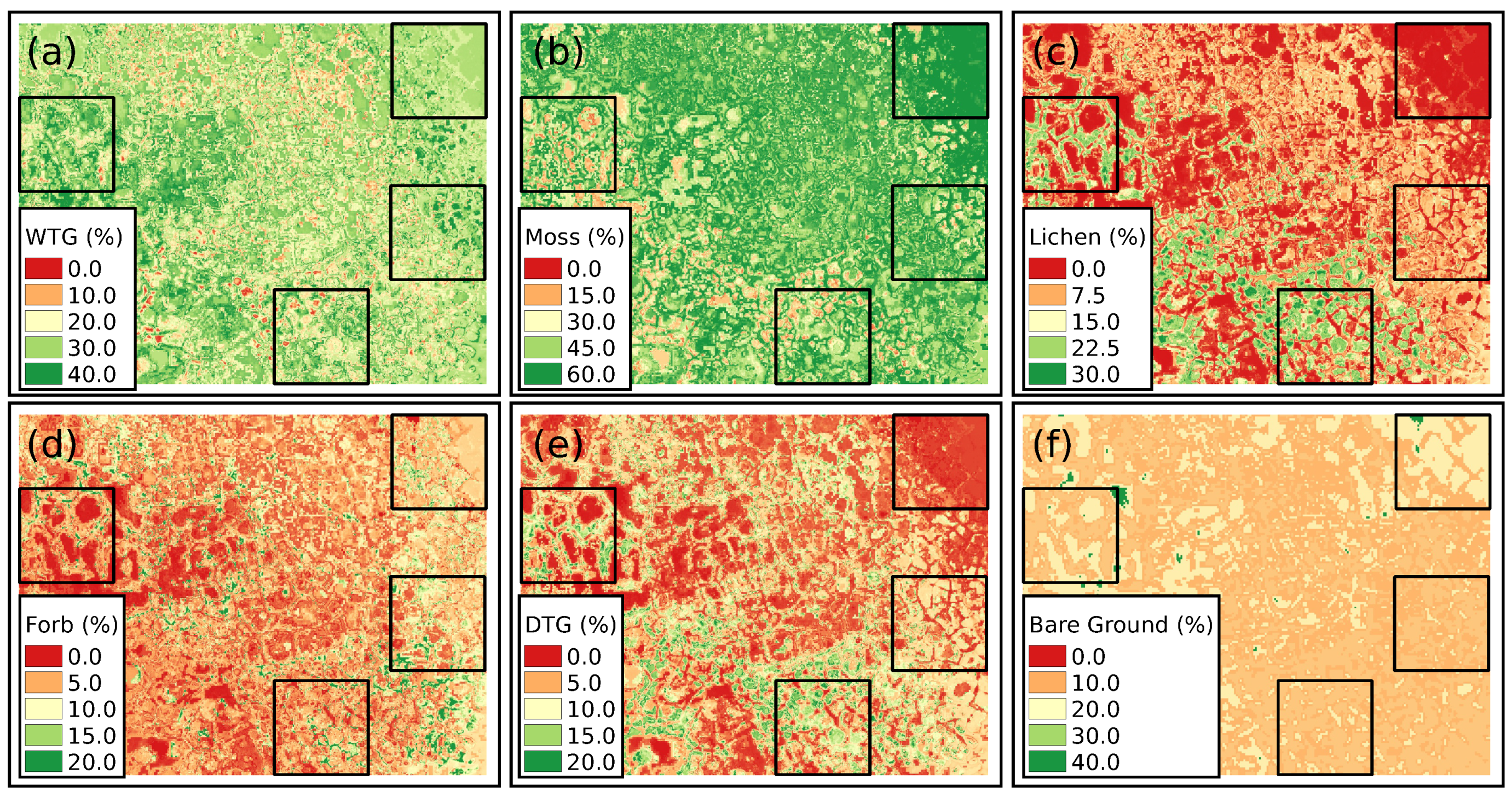
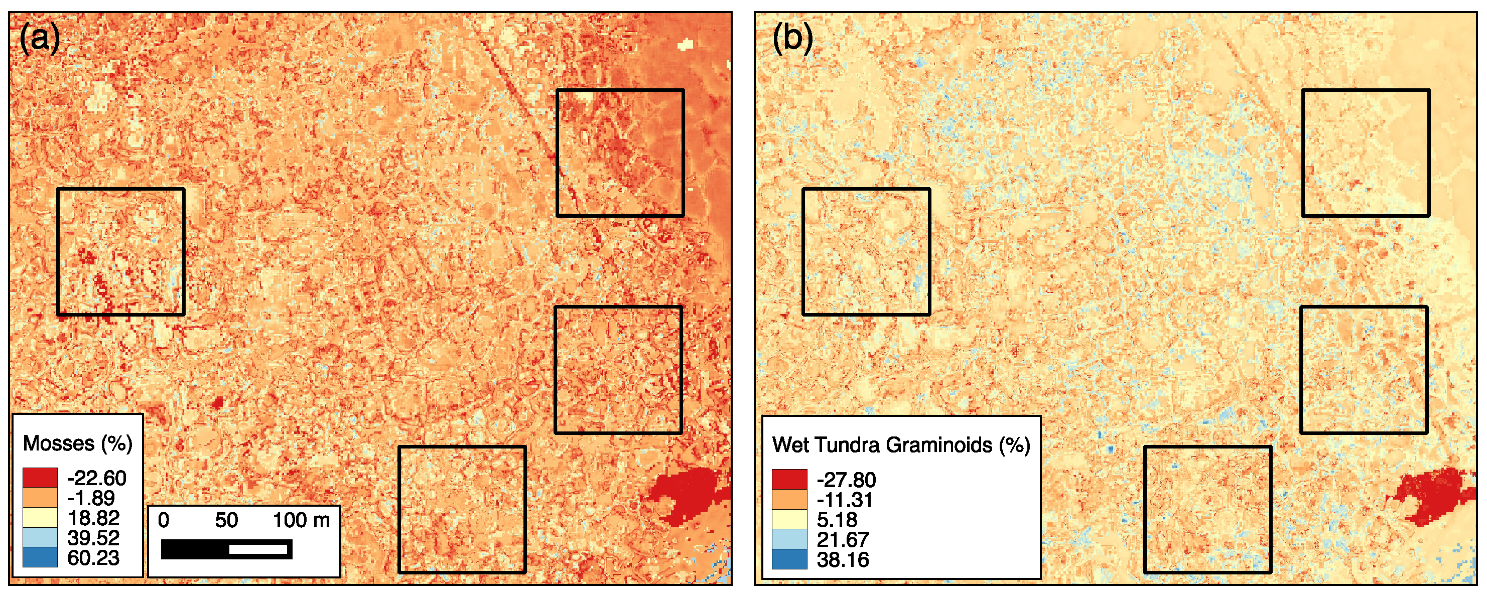
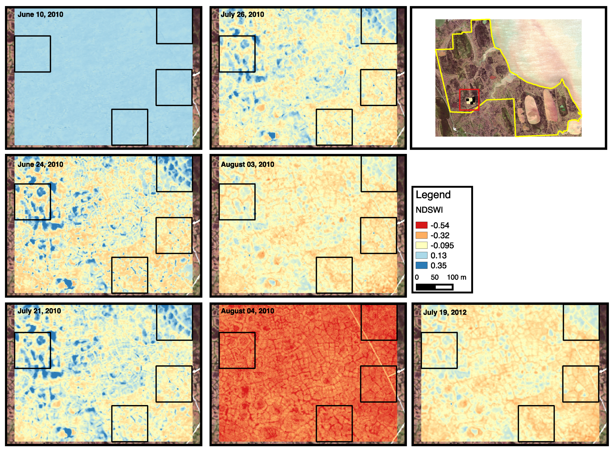
The IDW model was used for estimating wet tundra graminoids, dry tundra graminoids, forbs, mosses, lichens and bare ground. For the upscaled PFTs, percent cover greater than 100% refers to plot areas that have multiple layers of PFTs, while percent cover less than 100% refers to areas that have some cover of standing water or standing dead vegetation. The upscaled PFTs were rescaled to 100% and marked as standing water or standing dead vegetation for areas under 100%. The appendix describes how standing water was detected in the WorldView-2 satellite images and the associated impacts on the upscaled estimations.
2.5. Validation of PFT Upscaling
2.5.1. Bootstrap Validation
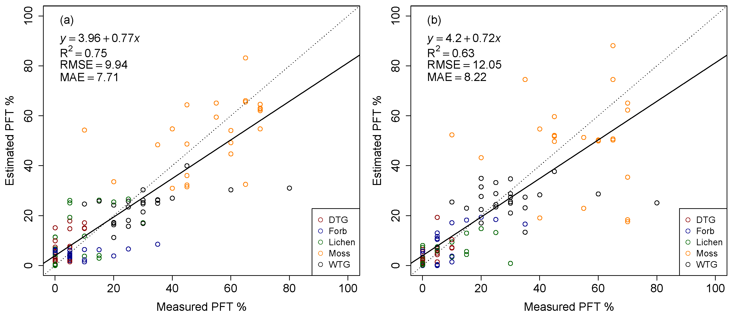
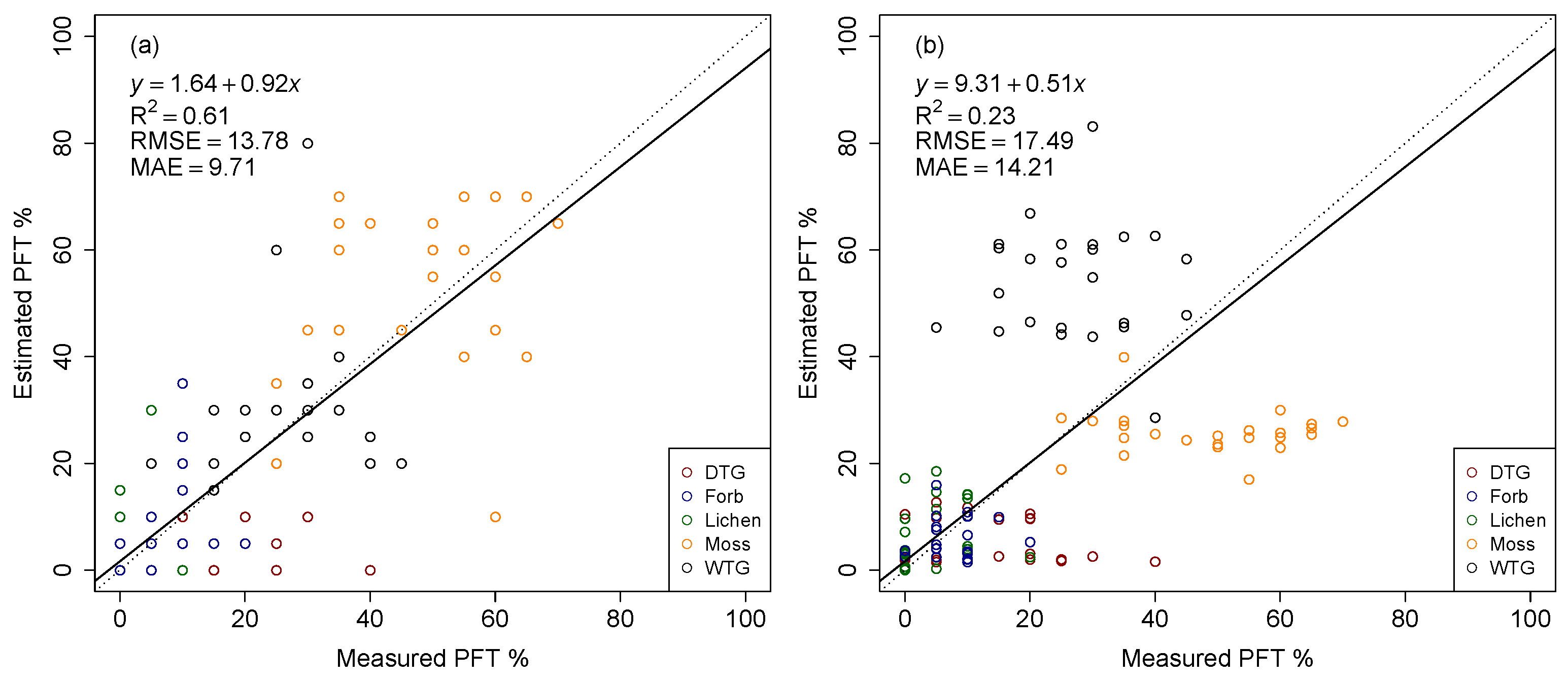
IDW was performed on for the with phenology and without phenology classifications. Bootstrap (random sampling) validation was used in order to evaluate how well IDW performed, which is essential due to the strong autocorrelation at the sampling location. Bootstrapping creates an unbiased set, where every possible combination of sampling units has an equal and independent chance of being selected. Forty eight random samples (25% of the plot corners) for wet tundra graminoids, dry tundra graminoids, forbs, mosses, lichens and bare ground (total of 288 samples) were taken out for running IDW for . This was performed for both the without phenology and with phenology cases. To allow for fair comparison, the same set of randomly-selected points was used for the validation of both the cases. After running the IDW model, the estimated PFT values at the 48 held back locations were extracted and compared against the observation.
2.5.2. Ground-Truthing
In addition to bootstrapping validation, an independent on-ground validation was performed by conducting a field survey on 29 July 2014. The locations for field samples were strategically selected based on the representativeness analysis (
Section 2.3). Within each sampling area (A, B, C and D), three locations that were well-represented by the original field samples (determined by representativeness metric) were selected for field sampling. In addition, we also selected three locations at each of the four areas that were under-represented by the original vegetation samples. Thus, a total of 24 1 m × 1 m plots was selected for field sampling for the validation of the upscaled PFT distribution products. High-resolution optical imagery was used to visually locate and extract plot coordinates across the various sampling areas. Similar to the 48 1 m × 1 m plots, the 24 plots were surveyed using a dGPS. Unlike the earlier survey of the vegetation composition, no attempt was made to identify species or genera, and only PFT measurements were made. Fractional area distributions of wet tundra graminoids, dry tundra graminoids, forbs, mosses and lichens were determined in these 24 1 m × 1 m plots. All plots were sampled close to the peak growing season.
We expect the accuracy of the estimated PFT distributions at the plots well-represented by the vegetation samples to be better compared to the plots that were under-represented. The representativeness metric helps identify the areas where additional observation can help improve the model. To test that hypothesis, we added the observation at 24 well- and under-represented plots to the IDW model training datasets and repeated the analysis to generate a new estimate of the PFT distribution. A second ground-truthing campaign was performed on 30 August 2014 at the same 24 plots using the same sampling strategy. Some senescence may have occurred by 30 August; however, it has been shown that the production of foliage can continue into late August in Barrow, AK [
45]. The second ground-truthing serves to evaluate the estimation error when additional observations at well- and under-represented plots are included in the model development based on the field campaign on 29 July 2014.
4. Discussion
High-resolution LiDAR and optical datasets are becoming more accessible, and new approaches for analyzing such datasets are valuable to improving knowledge of Arctic ecosystems. This study estimated the distribution of PFTs using multiple high-resolution satellite imagery captured during the 2010 growing season. We developed an approach that combines
k-means clustering [
42], representativeness [
31,
43], and interpolation methods for optimally using the sparse point measurements to develop continuous gridded PFT estimates; taking a different approach from previous studies.
WorldView-2 multispectral satellite imagery has a much higher resolution compared to commonly-used satellites (e.g., Landsat, MODIS, etc.) and captures the fine-scale variation in PFTs within a small sampling domain. Clustering the spectral and topographic characteristics together provided a systematic method for delineating the landscape and allowed for the development of better upscaling models using field observations from similar environment (in the multi-variate data space). We conducted cluster analysis for varying level of divisions (
) with the primary focus on stratifying the polygonal landscape. At our polygonal tundra sites with significant microtopography, cluster analysis at the
level of division provided the best stratification of the landscape (
Figure 4) and provided the highest correlation coefficient during the bootstrap validation. For application to a different landscape, the optimal level (
k) for clustering based stratification can be adjusted to appropriately capture the heterogeneity and features of interest.
Data from the vegetation surveys (mid-July 2012) and the first field ground-truthing campaign (late-July 2014) were very comparable, indicating similar vegetation conditions at the site during 2012 and 2014. The distribution of vegetation (PFTs) varies throughout the growing season, for example, early in the growing season standing biomass will be dominated by mosses and lichens, with the vascular plant component increasing as the season progresses [
46]. Data indicate that including multiple images during seasonal growth, thus capturing phenology, captured this variance in our upscaling model. Including the targeted field observations at well- and under-represented sites collected as part of field based validation significantly improved the accuracy of PFT estimates. However, the
was lower for the with phenology case (
Figure 12a) when compared to the first ground-truthing (
Figure 11a) exercise. Data show that the second ground-truthing campaign was conducted in late-August 2014, while most the PFTs were beginning the “brown-down” period. Specifically, our with phenology IDW model captured the “green-up” period during the 2010 growing season, and sufficient remote sensing data were not available to capture the “brown-down” period. Including more remote sensing images during the last part of the growing season would help capture the “brown-down” and, therefore, potentially further distinguish PFT distributions. Including the whole growing season in the PFT estimate may help represent dynamic PFTs for models.
IDW works well with high-resolution remote sensing datasets; in addition, by stratifying the landscape using cluster analysis and developing separate model with each cluster and using the observations within the cluster allowed for spectral similarity and, thus, better and specialized models. The results of this study are applicable to the regions with similar vegetation and spectral characteristics. Furthermore, this study is well suited for upscaling fine-scale measurements over areas similar to the BEO. For example, clouds may become an issue if one decides to study larger areas. However, the same approach could be applied to cloud-penetrating L-band Synthetic Aperture Radar or to a subset of imagery throughout the growing season.
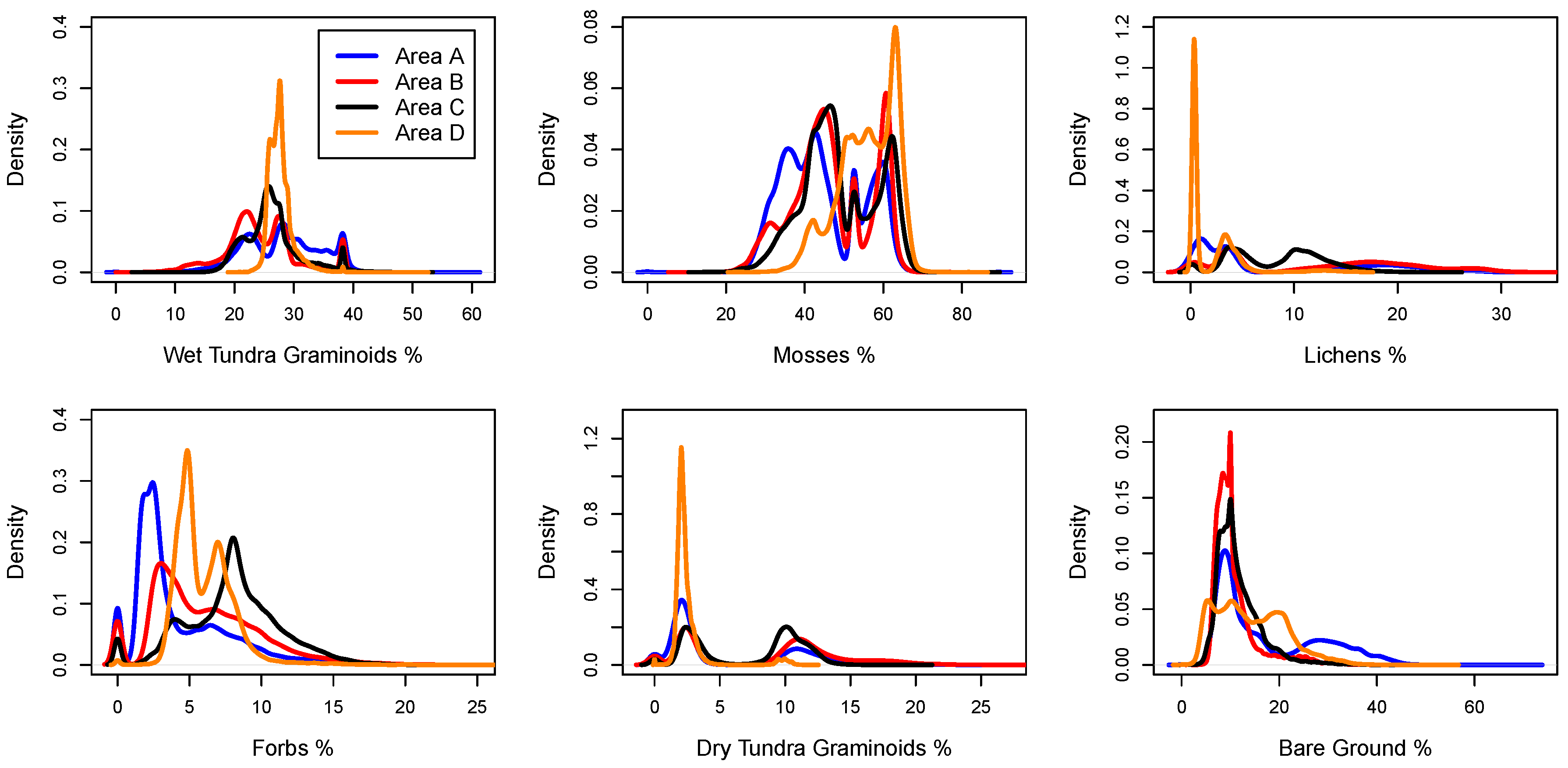
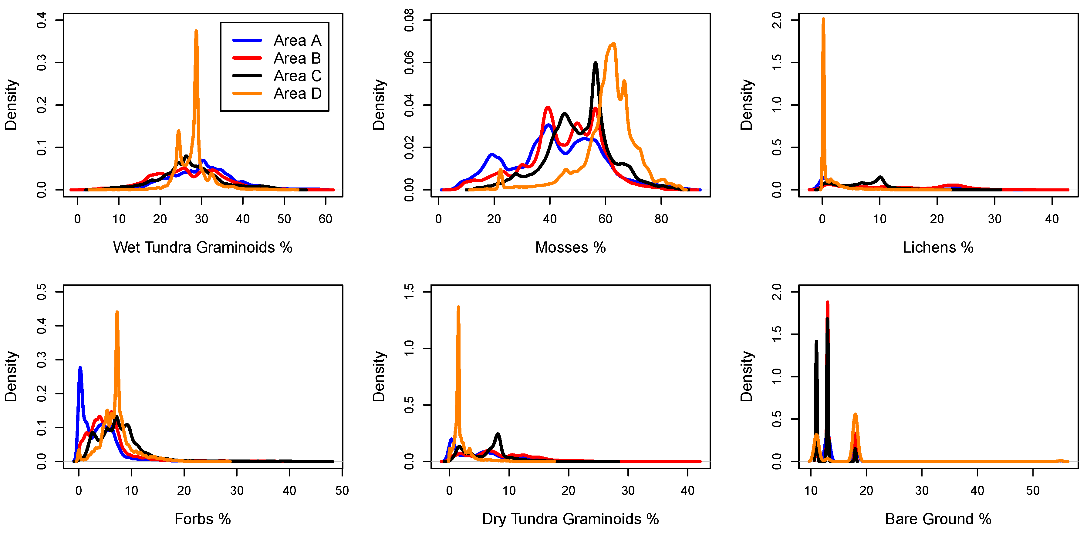
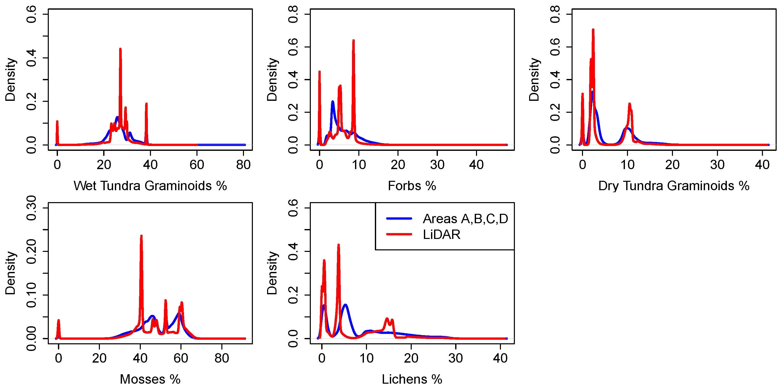
The distribution of PFTs for Areas A, B, C and D shows a multimodal distribution, which could be due to the polygonal types and features and was also attributable to how observers estimated plant distributions by multiples of 5% or 10% (
Figure 13). For example, higher wet tundra graminoid values were predicted for Area A (low centered polygons), while lower wet tundra graminoid values were predicted for Area B (high centered polygons). This attribution of microtopography can also be seen in other upscaling studies around Barrow, AK [
27]. For Arctic landscapes where the polygonal landscape are not the primary control, PFTs could depend on other criteria, such as the topographic position, and it is essential to find specific algorithms and model parameters with proper site-specific PFT measurements.
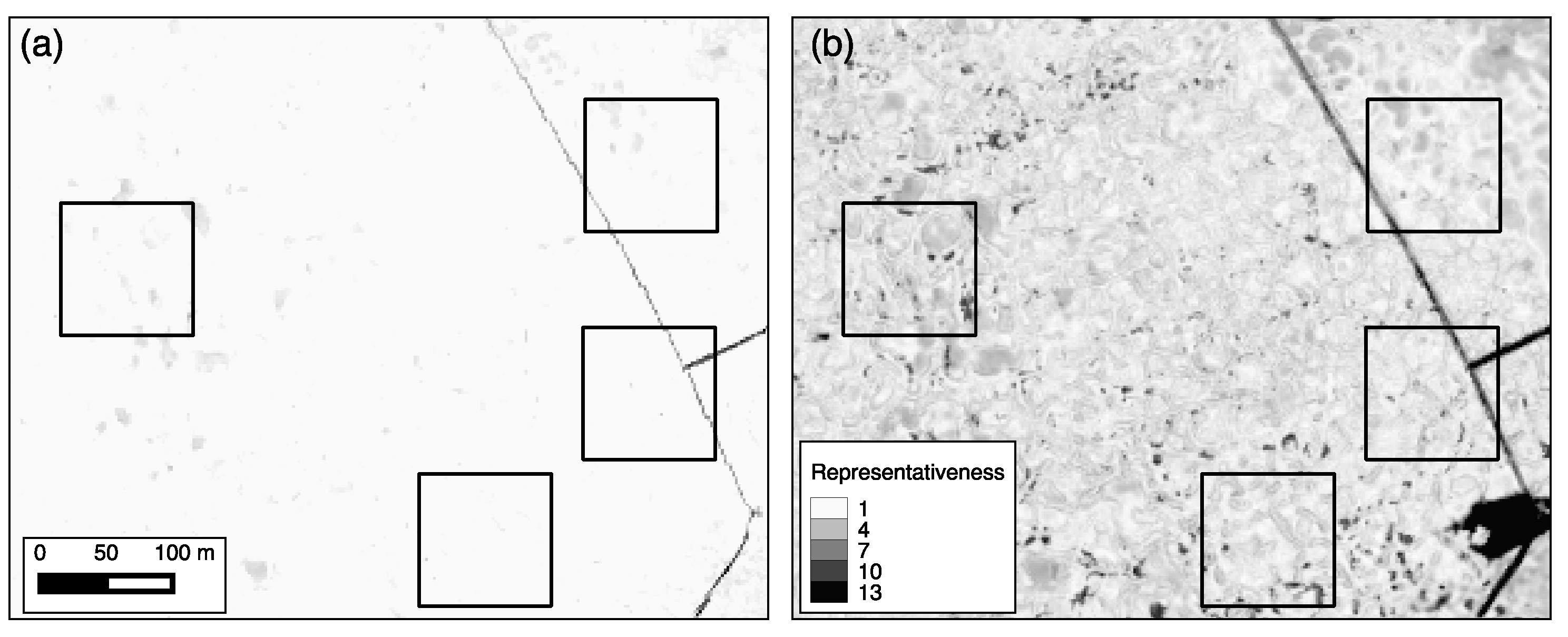
The Euclidean distance in the multi-variate state space provided a metric for representativeness. Gray-scaled representativeness maps showed the similarity of every map cell to the vegetation sampling locations in the BEO. This provided a sampling strategy to identify under-represented areas for further field sampling. Including additional observations from the under-represented areas in the IDW model significantly improved the estimation of PFT distributions across the landscape. This analysis can provide model-inspired insights into optimal sampling strategies across space and through time [
31]. The accuracy of the upscaled data were higher for areas well represented by the sampling sites and lower for areas that were under-represented. The difference maps from subtracting the with phenology and without phenology showed that the greatest differences occur in the poorly-represented areas (
Figure 10). These poorly-represented areas are due to differences in the spectral and topographic differences, meaning that different vegetation characteristics could occur in these areas. Furthermore, highly saturated areas could produce under-represented areas, and adding moisture content to the upscaling approach could improve PFT estimates. The improved representativeness analysis still shows locations that are under-represented and should be investigated in future field campaigns.
The methods we utilized here have improved our ability to predict the vegetation cover across broad portions of the landscape on the BEO. On-going research to improve the relationships among species-specific tundra vegetation cover, biomass and the allocation of carbon below-ground to the production of roots and rhizomes [
47,
48] may extend the utility of remote-sensing from observable plant and environmental characteristics to unobservable characteristics and processes beneath the soil surface. Other Arctic landscapes could benefit from our research by gathering the measurements mentioned above and applying these methods (i.e., representativeness, clustering, interpolation). However, one might want to test different multivariate statistical methods (i.e., linear regression, neural networks).
The remote sensing imagery was collected in 2010; the training data used were collected in 2012; and the ground-truthing was conducted in 2014. Changes in vegetation composition and cover do occur through time, but they are much slower in the Arctic tundra compared to other parts of the world [
20]. However, herbivory outbreaks can occur in the BEO. Villarreal et al. [
49] saw low amounts of biomass in 2008 for all communities caused by a lemming population outbreak. We are assuming that dramatic changes in PFT percentages did not occur for 2010, 2012 and 2014, since we had high coefficients of determination from the ground-truthing campaigns. In order to accurately verify this, more high-resolution satellite and aerial imagery would be needed for these years.
Terrestrial vegetation plays an important role in the dynamics of the Earth system through water and energy exchange and is a large source of uncertainty in models. Chapin et al. [
13] recommended the use of Arctic- and boreal-specific PFTs in vegetation models, which includes deciduous shrubs, evergreen shrubs, sedges, grasses, forbs,
Sphagnum moss, non-
Sphagnum moss and lichens. Estimates of PFT distribution from our study provide necessary inputs to model vegetation across larger landscapes for high-resolution land surface models (e.g., Arctic Terrestrial Simulator, PFLOTRAN). Efforts are underway to perform model simulations at the BEO and to assess the sensitivity of including these Arctic-specific PFT distributions. The presented approach for upscaling in situ measurements using high-resolution satellite imagery provides a framework for future studies focusing on Arctic ecosystem change.


 ,
, 


