2.1. Multiscale Segmentation of Difference Image
Due to impacts of sunlight, atmospheric condition and phenology cycle, it is difficult to obtain exactly corresponding objects by segmenting two temporal images individually. It discourages the comparison of objects, as uncertainties are accumulated when generating one-to-one correspondence. Therefore, two temporal images X1 and X2 are stacked into one image by simple band stacking, and segmentation is implemented on the stacked image.
Many clustering methods have been investigated to segment images, such as
k-means and iterative self-organizing data analysis techniques algorithm. The results depend on the initialization to a certain extent. Recently, statistical region merging (SRM) was proposed to segment images, which has the ability of removing significant noise, handling occlusions, and can perform scale-sensitive segmentations fast [
36]. Thus, SRM is adopted to segment the stacked image in this study.
The stacked image X contains m × n pixels, with each pixel containing 2L values, each of the 2L channels belonging to the set {0, 1, …, g}, and g = 255 here. Let X* denote the perfect segment scene of observed image X. Each channel of X is obtained by sampling each statistical pixel of X* from a set of exactly Q independent random variables (taking values within [0, g/Q]) for observed 2L channels. The tuning Q controls the scale of segmentation: the larger it is, the more regions exist in the final segmentation.
The SRM segments an image based on an interaction between a merging predicate and an order in merging. The merging predicate
can be expressed as follows
where
R and
denote a fixed couple of regions of
X,
and
are the average grey values for channel
a in region
R and
, respectively, and
(
). If
,
R and
are merged. The function
f of merging order used to sort pixel pairs in
X is described as
where
and
are pixels in
X, and
and
are the pixel grey values of channel
a. The SRM is then performed to segment the stacked image with different
Q values and multiscale segmentation maps are obtained.
2.2. Pixel-Based CD Using FCM
In this part, CVA is used to generate the difference image, and FCM clusters the difference image to produce a change map with memberships belonging to changed and unchanged parts. First, the change vector
can be calculated as follows
where
includes all the spectral change information between
X1 and
X2 for a given pixel. The modulus
of change vector
is computed using Equation (4), which is recorded as the final difference image
Xd.
The difference image Xd is then normalized to [0, 255] in order to avoid the instability and inconsistency among the data sets and supply a consistent input for the following FCM clustering.
Afterwards, FCM [
37] is implemented to cluster the difference image and detect changes. The membership probability
(
,
c is the cluster number), that is, the pixel
xj in the difference image belonging to the
i-th (
i = 1 or 2) cluster, is determined by minimizing the objective function
where
U = [
uij] is the membership probability matrix of
Xd, and
V = [
v1,
v2, …,
vc] is the matrix composed of
c central values. The membership probability
uij can be calculated using the following equation
In Equation (6),
vi is computed as follows
where
m is a weighting exponent. For most data, 1.5 ≤
m ≤ 3 leads to satisfactory results [
37]. It is set to 2 in this study, a widely used choice in many works [
7,
38].
An optimum solution can be obtained by updating U and V iteratively, and the iteration process is stopped when the number of iterations reaches a predefined maximum number or is achieved, where Vt and Vt−1 are the cluster center matrix in the t-th and (t−1)-th iteration and is a predefined threshold. Finally, an initial change map and the membership probability U of pixels in the difference image are produced and used for uncertainty analysis.
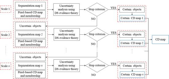
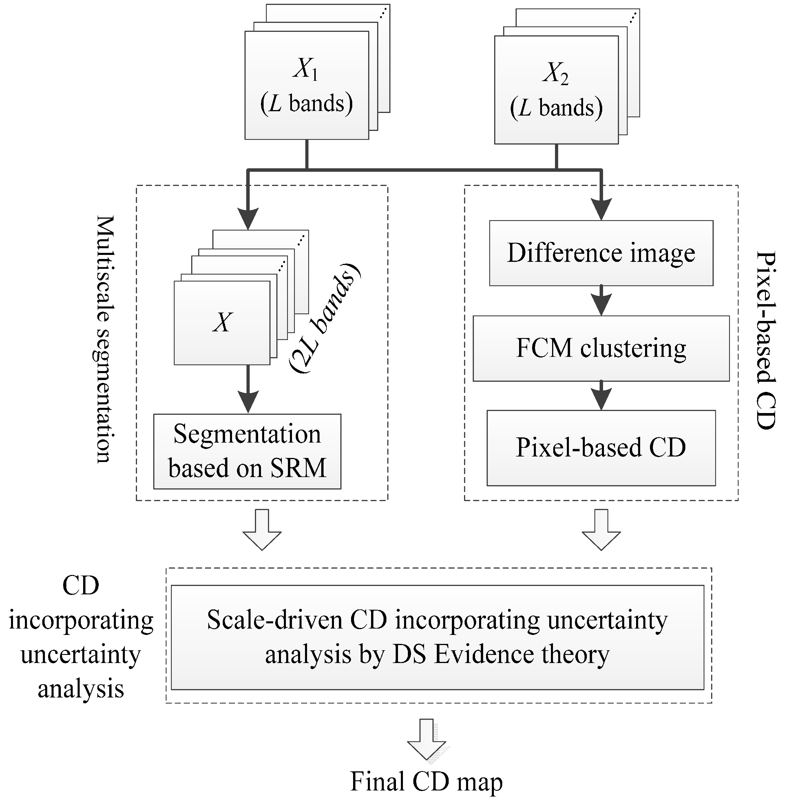
2.3. Scale-Driven CD Incorporating Uncertainty Analysis (SDCDUA)
In this study, a scale-driven solution is proposed to analyze the uncertainty existing in traditional CD, where DS evidence theory is employed, as shown in
Figure 2.
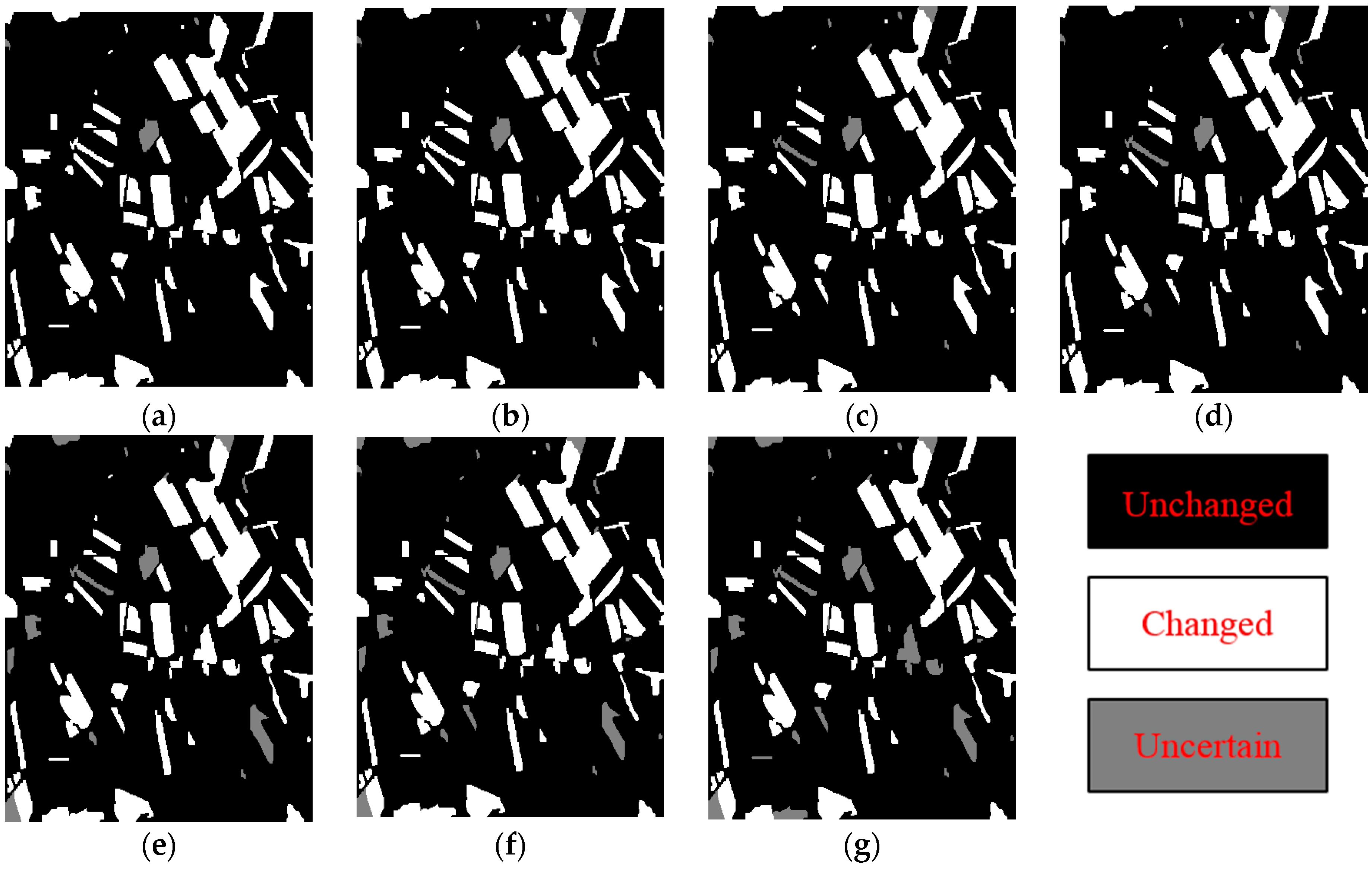
First, a coarse segmentation map of SRM is analyzed based on the pixel-based CD map and memberships. Then, it is classified into changed, unchanged, and uncertain parts through the uncertainty analysis using the DS evidence theory. More details of the DS evidence theory are introduced in the following content. Only certain changed and unchanged objects are included in ‘Certain CD map 1’ shown in
Figure 2. Second, for uncertain objects after the uncertain analysis, the next scale segmentation map with more detailed objects is adopted and analyzed with the pixel-based CD map and memberships. In this stage, the uncertain objects are also divided into changed, unchanged and uncertain parts, and a CD map consisting of identified changed and unchanged objects is also obtained, labeled as ‘Certain CD map 2’ in
Figure 2. Next, the uncertain parts are further analyzed as showed in the last stage, which iterates until no uncertain object exits or the final segmentation map has been utilized. Finally, all ‘Certain CD maps’ are combined together to generate the final CD map.
The main step of uncertainty analysis based on DS evidence theory in SDCDUA is presented as follows. The DS evidence theory is an extension of the traditional Bayesian theory. The theory was first introduced by Dempster [
39] in the context of statistical inference, and it was later extended to a general framework for modeling epistemic uncertainty by Shafer [
40]. Three important functions in DS theory are defined and used to model the uncertainty, namely, the basic probability assignment function (
m), the Belief function (
Bel), and the Plausibility function (
Pls).
Let
be the space of hypothesis and
denote the set of subsets of
. For any hypothesis
A of
,
m(
A) ∈ [0, 1] and
where ∅ represents the null set,
m is the basic probability assignment function (BPAF), and
m(
A) denotes the basic probability of the hypothesis
A.
Generally, the belief degree of the combined result from different evidences is represented with an interval. The upper and lower limits of the interval are called the Belief function (
Bel) and the Plausibility function (
Pls), respectively, which are computed as follows
where
A and
B are made up of several or all the elements in
,
, and the values of
Bel and
Pls range from [0, 1].
A new evidence
m(
c) is then calculated by fusing different source evidences using the following equation
where
denotes the fusion of evidences, and
m1,
m2, …,
mn are the basis probability assignment function.
In CD problem,
, where
C denotes “change” and
U represents “no-change”. Two evidences are generated and combined in this study. One is the object-based evidence
produced based on the segmentation maps, and the other is the pixel-based evidence
obtained with FCM. First, objects in a segmentation map are partitioned into changed and unchanged parts by minimizing the difference of grey values of pixels in each part, and the mean values of changed and unchanged parts are calculated. For an object
Ri, its variances corresponding to changed and unchanged parts are obtained and termed
and
, respectively. Thus, the evidence
of the object
Ri can be obtained with the following equation
where
and
are probabilities of the object
Ri belonging to changed and unchanged parts in the first evidence, respectively.
The second evidence
of the object
Ri is calculated from the membership of pixels belonging to changed and unchanged parts with the following equation
where
and
are probabilities of the object
Ri belonging to changed and unchanged parts in the second evidence, respectively, and
n is the total number of pixels in the object
Ri.
and
are probabilities of the
j-th pixel belonging to changed and unchanged parts in the object
Ri, respectively. They are computed by clustering the difference image using FCM algorithm in
Section 2.2.
The evidences
and
are then combined into a new evidence
, where
and
are probabilities of the object
Ri belonging to changed and unchanged parts in the new evidence, respectively. For example,
and
.
k can be calculated using Equation (11) as
The
Pc of the new evidence is calculated as
The
Pu of the new evidence is computed as
A threshold
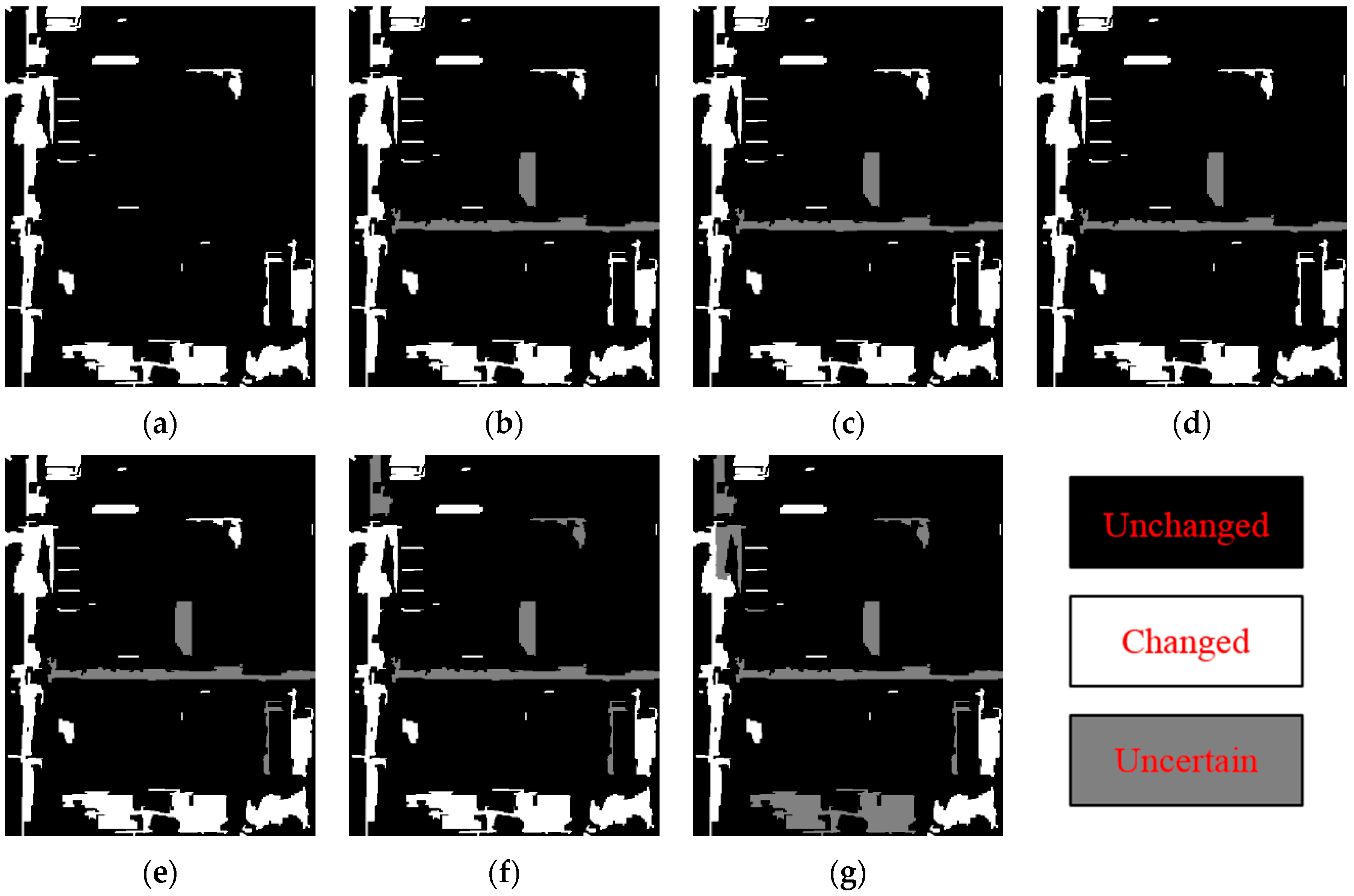
is then set to classify the object into unchanged, uncertain and changed groups with the following equation
where
li = 1, 2, 3 denote that the object
Ri belongs to changed, changed and uncertain groups, respectively.
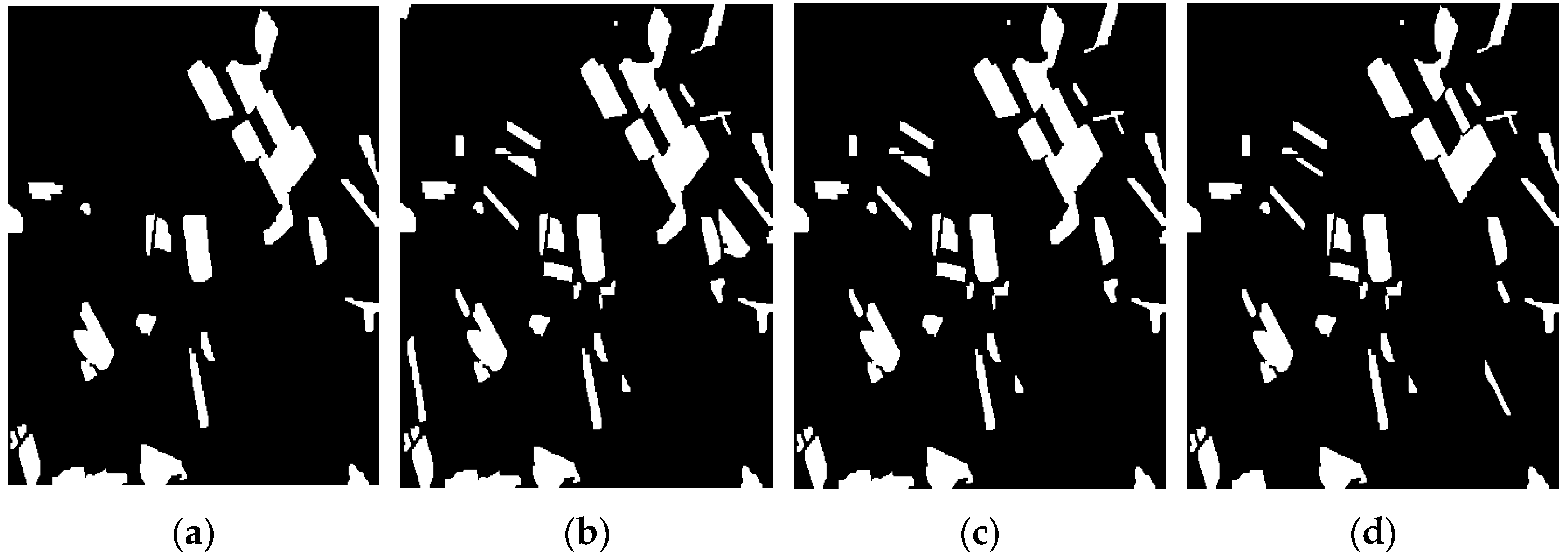
After the uncertainty analysis using DS evidence theory based on multiscale segmentation maps and pixel-based CD, a final change map can be obtained. For quantitative assessment on CD results, several indices are adopted: (1) Missed detections Nm that indicate the number of incorrectly classified unchanged pixels in the CD map. The ratio of missed detections Pm is calculated by , where N0 is the total number of changed pixels counted in the ground reference map; (2) False alarms Nf that indicate the number of the incorrectly classified changed pixels in the CD map. The ratio of false alarms Pf is calculated with the ratio , where N1 is the total number of unchanged pixels counted in the ground reference map; (3) Total errors Nt that indicate the total number of detection errors, including both missed and false detections. This total number refers to the sum of missed detections and false alarms. Hence, the ratio of total errors Pt is calculated with .


