Exploring the Potential of Active Learning for Automatic Identification of Marine Oil Spills Using 10-Year (2004–2013) RADARSAT Data

Abstract

This paper intends to find a more cost-effective way for training oil spill classification systems by introducing active learning (AL) and exploring its potential, so that satisfying classifiers could be learned with reduced number of labeled samples. The dataset used has 143 oil spills and 124 look-alikes from 198 RADARSAT images covering the east and west coasts of Canada from 2004 to 2013. Six uncertainty-based active sample selecting (ACS) methods are designed to choose the most informative samples. A method for reducing information redundancy amongst the selected samples and a method with varying sample preference are considered. Four classifiers (k-nearest neighbor (KNN), support vector machine (SVM), linear discriminant analysis (LDA) and decision tree (DT)) are coupled with ACS methods to explore the interaction and possible preference between classifiers and ACS methods. Three kinds of measures are adopted to highlight different aspect of classification performance of these AL-boosted classifiers. Overall, AL proves its strong potential with 4% to 78% reduction on training samples in different settings. The SVM classifier shows to be the best one for using in the AL frame, with perfect performance evolving curves in different kinds of measures. The exploration and exploitation criterion can further improve the performance of the AL-boosted SVM classifier but not of the other classifiers.

1. Introduction

With the increase of maritime traffic, the accidental and deliberate discharge of oil from ships is attracting growing concern. Using satellite-based synthetic aperture radar (SAR) has been proven to be a cost effective way to survey marine pollution over large-scale sea areas [1,2].

Current and future satellites with SAR sensors that can be used for monitoring oil spills include ERS-1/2, RADARSAT-1/2, ENVISAT (ASAR), ALOS1/2 (PALSAR), TerraSAR-X, Cosmos Skymed-1/2, RISAT-1, Sentinel-1, SAOCOM-1 and the RADARSAT constellation mission. Based on the SAR systems, many commercial or governmental agencies have been building SAR oil-spill detection service, such as the multi-mission maritime monitoring services of Kongsberg Satellite Services (KSAT), Airbus defense and space’s oil spill detection service, CleanSeaNet [3] and Integrated Satellite Tracking of Pollution (ISTOP). To be more operational, automatic oil spill classification system with real-time, fully operational and wider water coverage capability is needed [1], as Solberg et al. state [4] “The currently manual services is just a first step toward a fully operational system covering wider waters”.

Due to their ability to smooth sea surface, oil spills usually appear as dark spots on SAR images. However, other sea features, such as low wind areas and biogenic slicks, also produce smooth sea surface and result in dark formations on SAR imagery. These sea features are usually called “look-alikes”. The existence of look-alikes imposes huge challenge on SAR oil spill detection systems. In an automatic or semiautomatic SAR oil spill detection system, three steps are sequentially performed to identify oil spills [1,5,6,7,8]: (i) dark-spot detection for identifying all candidates that belong to either oil spills or look-alikes; (ii) feature extraction for collecting object-based features, such as the mean intensity value of dark-spots, for discriminating oil spills and look-alikes; and (iii) classification for separating oil spills and look-alikes using the features extracted.

After identifying all candidates and collecting their features, classification approaches predominantly determines the performance of oil spill detection systems. Many classifiers have been used to detect oil spills including a combination of statistical modeling and rule-based approaches [1,4,5,9,10], artificial neural network (ANN) models [11,12,13,14,15,16], decision tree (DT) models [3,8,15,17], fisher discrimination or multi regression analysis approaches [18], fuzzy classifiers [3,19], support vector machine (SVM) classifiers [9,20] and K-nearest neighbors (KNN) based classifiers [17,21]. A comparison of SVM, ANN, tree-based ensemble classifiers (bagging, bundling and boosting), generalized additive model (GAM) and penalized linear discriminant analysis on a relatively fair standard has been conducted [22] with the conclusion that the tree-based classifiers, i.e., bagging, bundling and boosting approaches, generally perform better than the other approaches, i.e., SVM, ANN and GAM.

Most classifiers that have been adopted for oil spill detection are supervised classifiers which need training samples to “teach” themselves before performing classification tasks. To get good generalization performance, a large number of training samples are needed to deal with the curse of dimensionality [23]. In the case of oil spill classification, high feature dimensionality are usually needed to cover the complex characteristics of look-alikes and oil spills [1,6].

Although effective classifier learning requires a large number of labeled samples, verifying/labeling and accumulating enough number of samples for training an automatic system with reasonable performance could be very difficult, costly and time-consuming for the following reasons. First, oil spills are rare and fast-changing events, which tend to disappear before being verified by ships or aircrafts, because, after a short time span, mostly within several hours [24], the oil spills will become difficult to distinguish. Second, verifying an oil spill using airplane/vessel is usually very expensive. Third, verified/labeled samples from different SAR platforms may not be sharable, because of the different imaging parameters, such as band, polarization mode, spatial resolution, etc. Even for images from the same SAR platform, the standards of confidence levels, pre and post procedures, etc. must be normalized so that the samples from different institutions can be shared.

Limited by difficulties in verifying oil spills, researchers rely mainly on human experts to manually label the targets. For example,

Table 1. Summary of the dataset adopted in different SAR oil spill detection researches. Note that in the #samples column; (X, Y) indicates there are X oil spills and Y look-alikes and, in the #Samples verified column; (X, Y) indicates there are X verified oil spills and Y verified look-alikes.

Literature	SAR Sensor	#Image	#Samples	#Samples Verified	Location (Time Span)
[22]	RADARSAT1	93	(98, 94)	(21, N/A)	West and East coasts of Canada (2004–2008)
[9]	Envisat	103	(41, 12, 245)	N/A	Baltic Sea and North See (2003–2005)
[10]	Envisat RADARSAT1	127	(37, 12, 110)	(29, N/A)	Baltic Sea and North See (2003–2004)
[4]	Envisat	84	(71, 6980)	N/A	European waters (N/A)
[7,8,12,13,14]	ERS-2	24	(69, 90)	N/A	Mediterranean Sea (N/A)
[19]	ERS-1/2	12	N/A	N/A	Mediterranean Sea (N/A)
[24]	ERS-1/2	1600	(1638, N/A)	N/A	Mediterranean Sea (1999)
[18]	ERS-1/2 Envisat	N/A	(153, 237)	N/A	Mediterranean Sea (N/A)
[26]	ERS-1/2 Envisat	15, 533	(9299, N/A)	N/A	Mediterranean Sea (1999–2004)
[26]	ERS-1/2 Envisat	3165	(1227, N/A)	N/A	Black sea (1999–2004)
[15]	Envisat	47	(80, 155)	N/A	Galicia coast, Spain (2007–2011)
[3]	Envisat RADARSAT	118	(361, 5728)	N/A	European Waters (2009–2012)
[17]	ERS-1 RADARSAT1	9	(41, 896)	N/A	N/A

indicates that the largest number of verified oil spills is only 29 adopted by Solberg et al. [10], and other researchers predominantly used the expert-labeled samples, although they did not explicitly report the proportion of the verified samples. Nevertheless, using expert-labeled samples is problematic for the following reasons. First, expert-labeling produces inconsistency between the labels (or confidence levels) given by different experts [1,25]. Second, training the system with expert-labeled samples leads to system that can hardly outperform the experts who “teach” the system.

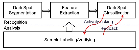
Considering the cost and difficulties in verifying oil spill candidates, one key issue in learning an oil spill classification system is to effectively reduce the number of verified samples required for classifier training without compromising the accuracy and robustness of the resulting classifier. Suppose that the current verified samples are insufficient for building an accurate oil spill detection system, and that new samples are required to be verified for increasing the size of the training set. In a conventional supervised classification system, we will not be able to know which samples have higher priority to be verified, because, as indicated in Figure 1, the communication between the conventional classification system and the sample collecting system is one-way directed, where the collected samples are used to train the classifier with no feedback from the classifier on what kind of samples are more informative and urgently needed. Without knowing the values and importance of the samples to the classifiers, the costly verification effort may only lead to training samples that are redundant, useless or even misleading. Although verifying more samples can increase the possibility of obtaining relevant training sample, it will greatly increase the time span and cost for building the system.

The need for reducing training samples without compromising the accuracy of resulting classifiers motivates us to study the potential of introducing AL into the oil spill detection systems. AL is a growing area of research in machine learning [27], and has been widely used in many real-world problems [27,28,29] and remote sensing classification [30,31,32,33,34,35,36]. The insight from AL is that allowing a machine learning algorithm to designate the samples for training could make it achieve higher accuracy with fewer training samples. As indicated by Figure 1, in an AL-boosted system, the interaction between the classification system and the training sample collecting system are bi-directional, where the classifier will “ask for” the most relevant samples to be verified/labeled in order to construct the classifier in an efficient and effective manner. Considering the cost and difficulty to verify the oil spill candidate, such an active learning process can greatly reduce the cost and time for building a detection system by reducing the number of candidates that needed to be verified without compromising the robustness and accuracy of the resulting classifier.

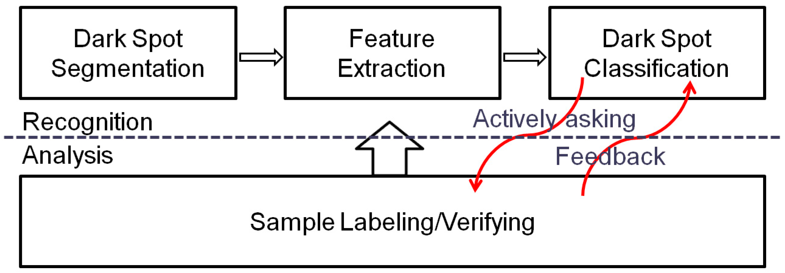
In this paper, we explore the potential of AL in training classifiers for the purpose of oil spill identification using 10 years (2004–2013) of RADARSAT data off the east and west coasts of Canada, which contains 198 RADARSAT-1 and RADARSAT-2 ScanSAR full scene images. Based on these images, we obtain 267 labeled samples, of which there are 143 oil spills and 124 look-alikes. We split these labeled samples into a simulating-set and a test-set, using the simulating-set to simulate an AL process involving a number of AL iterations, and using the test-set to calculate the performance of classifiers in each iteration. We start with a small number of training samples for initializing the classifiers, and with the AL iteration, we progressively select more samples and add them to the training set. Such a process ends when all samples in the simulating-set has been selected. Since the most important issue in AL is how to effectively select the most informative samples, we design six different active sample selection (ACS) methods to choose informative training samples. Moreover, we also explore the ACS approach with varying sample preference and the approach to reduce information redundancy among the selected samples. Four commonly used classifiers (KNN, SVM, LDA and DT) are coupled with ACS methods to explore the interaction between classifiers and ACS methods. Three kinds of measures are adopted to highlight different aspect of classification performance of these AL-boosted classifiers. Finally, to reduce the bias caused by the splitting of simulating set and test set in an effective manner, we adopt a six-fold cross validation approach to randomly split the labeled samples into six folds, using five for simulating and one for testing until all the folds have been used for testing once. To our best knowledge, this work is the first, effort except our very preliminary work [37], to explore the potential of AL for oil spill classification.

2. Dataset and Methods

The scheme of exploring the potential of AL for identifying marine oil spill is as Figure 2. In preprocessing step, the labeled samples are split into three parts. One part is put into the training samples pool for initially training classifiers. One part is put into the sample selection pool for sample selection in AL process. The third is for testing the performance of AL-boosted classifiers. The AL-boosted process starts by training classifiers with samples in the training sample pool. Samples in the sample selection pool are then classified by the trained classifiers, whose output are used to help the ACS approach to select some (here we select ten) most “informative” samples from the sample selection pool. These selected samples are added into the training samples pool to train classifiers in next iteration. The process keeps iterating until no sample left in the sample selection pool and all samples have been used to train the classifiers. We adopt four classifiers (i.e., SVM, LDA, KNN and DT), with each one coupled with all of the different ACS approaches. Three complementary numerical measures are calculated for each AL-boosted classifier using the testing set. The six-fold cross validation technique is used to get bias-reduced measures.

2.1. Dataset

The dataset used in this study contains 198 RADARSAT (188 RADASAT-1, 10 RADASAT-2) images (mode: ScanSAR narrow beam; swath width: 300 km; pixel spacing: 50 m) covering the east and west coasts of Canada from 2004 to 2013. Contained in these images are 143 oil spills and 124 look-alikes, all labeled by human experts in CIS of Environment Canada for a program called Integrated Satellite Tracking of Pollution (ISTOP). Because the boundaries of all labeled dark spots have been drawn by experts in CIS, we will not perform the dark spot detection process. Given the dark-spots in pixel-format, features extracted as input to classifiers can be categorized into four groups: (i) physical properties; (ii) geometric shape; (iii) texture; and (iv) contextual information [1,6,8]. Choosing the most relevant feature set for classification is not easy, because of the fact that feature selection is a complex issue depending on many factors such as the study area, the dataset, the classifiers, and the evaluation measures. Many researchers tried to study the relative importance of features for feature selection, but their conclusions are not in consistency due to their different experiment settings. For example, Karathanassi et al. [19] grouped 13 features into sea state dependent features and sea state independent features; Topouzelis et al. [7,8] examined 25 most commonly used features based on neural networks and decision tree forest, and selected several feature-subsets that are of most importance; Mera et al. [15] applied principal component analysis (PCA) to 17 shape related features and finally selected 5 principal components for their automatic oil spill detection system; and Xu et al. [22] implemented the permutation-based variable accuracy importance (PVAI) technique to evaluate feature’s importance relative to different criteria and they found that different types of classifier tended to present different patterns on feature ranking and PVAI values.

Due to the lack of unified criteria for feature selection, we decided to use as many relevant features as could be extracted. We finally obtained 56 features, of which, there are 32 features about physical properties, 19 features about geometric shape, and 5 features about texture characteristics (see

Table 2. Features extracted based on the dark-spot objects for classifying oil spills from look-alikes.

No	Type	Features	Code
1	Geometric	Target area in number of pixels	A
2		Target perimeter in number of pixels	P
3		Target Complexity measure C1 = P^2/A	C1
4		Target Complexity measure C2 = P/A	C2
5		Target Complexity measure C3 = P/(2*sqrt(pi*area))	C3
6		The length of the major axis of the ellipse that has the same normalized second central moments as the object region.	Length
7		The length of the minor axis of the ellipse that has the same normalized second central moments as the object region.	Width
8		The eccentricity of the ellipse that has the same second-moments as the object region	Ecce.
9		Target Spreading measures S = Length/Width	S
10–12		The first three of Hu's invariant planar moments [41]	H1–H3
13–19		The first seven of Zernike moments [42]	Z1–Z7
20	Physical	Average intensity value of the object	MeO
21		Standard deviation of gray-scale intensity values of the object	SDO
22		Average intensity value of the background area (a limited area near and outside object)	MeB
23		Standard deviation of the intensity value of the background area	SDB
24		Maximum intensity value of the object	MaxO
25		Minimum intensity value of the object	MinO
26		Power-to-Mean Ratio of the Object, SDO/MeO	PMRO
27		Power-to-Mean Ratio of the Background area, SDB/MeB	PMRB
28		Ratio between MeO and MeB	MeR
29		Ratio between SDO and SDB	SDR
30		Ratio between PMRO and PMRB	PMRR
31		Difference between MeB and MeO	MeD
32		Difference between SDB and SDO	SDD
33		Difference between PMRB and PMRO	PMRD
34		The difference between MeB and MinO	MaxC
35		Average gradient value of the object area	MeGO
36		Standard deviation of the gradient value of the object area	SDGO
37		Average gradient value of the background area.	MeGB
38		Standard deviation of the gradient value of the background area	SDGB
39		Average gradient value of the object border area.	MeGBo
40		Standard deviation of the gradient value of the object border area	SDGBo
41		Maximum gradient value of the object	MaxGO
42		Minimum gradient value of the object	MinGO
43		Ratio between SDGO and MeGO	PMRGO
44		Ratio between SDGB and MeGB	PMRGB
45		Ratio between MeGO and meGB	MeGR
46		Ratio between SDGO and SDGB	SDGR
47		Ratio between PMRGB and PMRGO	PMRGR
48		Difference between MeGB and MeGO	MeGD
49		Difference between SDGB and SDGO	SDGD
50		Difference between PMRGB and PMRGO	PMRGD
51		Difference between MeGB and MinGO	MaxGC
52	Textural	GLCM Contrast	Cont.
53		GLCM Correlation	Corr.
54		GLCM Energy	Ener.
55		GLCM Homogeneity	Homo.
56		GLCM Entropy	Entr.

). Wind and ship information that describe the contextual information of the identified objects are not included because these information and techniques needed to detect them are not available to us. Readers could refer to Solberg et al. [4] for manually setting wind information, Espedal et al. [38] for using wind history information and Hwang et al. [39] and Salvatori et al. [40] for automatic wind information detection from SAR images. The features used in this study have varying ranges of values. We normalize these features by linearly mapping the values from their ranges to [0, 1].

2.2. Classifiers Used

Four commonly used classifiers (SVM, KNN, LDA and DT) are adopted to be integrated into the AL framework. We prefer choosing commonly used classifiers in our study because: (i) we are focusing on exploring the effectiveness of the AL approaches, rather than finding the best classifiers; (ii) complex classifiers introduce more hyper-parameters that may complicate the performance, making it difficult to analyze the role of active learning; and (iii) conclusions drawn from commonly used classifiers may apply on high-level classifiers built on them, while it is not true vice versa. We set the hyper parameters of each classifier fixed across all AL learning iterations.

2.2.1. Support Vector Machine (SVM)

SVM is a “local” classifier whose decision boundary depends on a small number of supporting vectors/samples, which means finding the most relevant set of samples via AL is crucial for the performance. It is a well-known classifier for remote sensing applications [33,43] and particularly for oil spill classification [9,20,22]. Here, we use LIBSVM [44], the radial kernel, C = 1 and gamma = 0.07.

2.2.2. K Nearest Neighbors

KNN classifies a sample by a majority vote of this sample’s k nearest neighbors. It is widely used in remote sensing society [45,46,47] and particularly for oil spill classification [17,21]. We here simply set the only hyper parameter k = 9.

2.2.3. Linear Discriminant Analysis

LDA predicts the class membership based on the posterior probabilities of different classes. It assumes that the densities of predictors conditioned on class membership are Gaussian. Many modifications of LDA exist, such as Penalized LDA [48], null-space LDA [49], Dual-Space LDA [50], Probabilistic LDA [51], Global-local LDA [52], etc. Nirchio et al. [18] used LDA and Xu et al. [22] used the Penalized LDA directly for oil spill classification. Here, we use the basic LDA, hoping that conclusions drawn from LDA could apply to the other variants.

2.2.4. Decision Tree

DTs are flexible classifiers that recursively split the input dataset into subset [53]. The class label of a test sample is predicted by applying the decision criteria from the root to the leaves to determine which leaf it falls in. Because of its capability of easily providing an intelligible model of the data, decision tree is very popular and widely used for classification purpose either directly [3,15] or as the elemental classifier of state-of-the-art ensemble techniques such as bagging, bundling and boosting for achieving better generality performance [8,22,54,55,56]. Here, we use the DT supported by the classification and regression tree (CART) algorithm [53]. ClassificationTree class in Matlab 2012b was used, with all parameters set as default.

2.3. Active Learning

The AL process iteratively helps the classifier to identify and adopt the most informative samples for training the classifier in an efficient and effective manner. In each iteration, a classifier is first trained with current training set, then active sample selecting (ACS) methods choose L (here L = 10) samples that are most informative for current classifier, obtain their labels and add them to the training set. The ACS method responsible for informative sample selection is of key importance to the success of the AL process. To explore the influence of different ACS methods on the classifier performance, here, we choose the uncertainty criterion to define the informativeness of samples and design six basic ACS methods based on it. Two strategies that may further improve the informativeness of the selected samples by adjusting sample preference in iterations and reducing redundancy amongst samples are also considered.

2.3.1. Six Basic ACS Methods

We choose the most widely used uncertainty/certainty criterion for describing the informativeness of samples [27] and propose six ACS methods based on it. Here, the certainty of a sample being an oil-spill is defined by its posterior probability that is usually implemented as the soft-outputs of classifiers. For KNN classifier, the posterior probability of input x, is defined as $p\left(oil\right|x)=\#(oilspillsinN\left(x\right))/K$, where N(x) is the K nearest neighbors of x. For LDA classifier, it is defined as $p\left(oil\right|x)=\propto p(x\left|oil\right)$, where $p\left(x\right|oil)$ is a multivariate normal density trained by LDA. For SVM classifier, we use libSVM toolkit [44] which obtains the probability according to the work of Wu et al. [57]. Traditionally, DT can only provide piecewise constant estimate of the class posterior probabilities, since all the samples classified by a leaf share the same posterior probabilities. Some improvements have been proposed [58] for getting a more smooth estimation of the class posterior probabilities. For simplicity, we here still use the traditional estimation, i.e., posterior probability of input x classified by a leaf, is defined as $p\left(oil\right|x)=k/n$, where k is the number of training samples being classified into the oil spill class by the leaf, and n is the total number of training samples being classified by the leaf.

Sorting all samples in the sample selection pool according to their certainty of being oil spills $p\left(oil\right|x)$, their certainty of being look-alikes 1 − $p\left(oil\right|x)$ and their uncertainty of classification 1 − $abs(0.5-p(oil\left|x\right))$ in descending order, we obtain three sequences, which are denoted by q1, q2 and q3, respectively.

Let L be the number of samples selected in each iteration of active learning, and w1, w2 and w3 be the percentages of samples that will be selected from q1, q2 and q3, respectively. Then, our ACS algorithm here can be denoted with ACS(w1,w2,w3), where w1 + w2 + w3 = 1. It means at each iteration, our algorithm selects respectively w1*L, w2*L and w3*L samples from q1, q2 and q3 with no replicates. All the selected samples are then labeled and put into training sample set. We design here our ACS methods according to the different setting of (w1, w2, w3) in

Table 3. Six basic active sample selecting (ACS) methods.

Method	Parameters	Description
ACS-1	NULL	Randomly select samples
ACS-2	w1 = 1, w2 = 0, w3 = 0	Prefer samples more like oil spills
ACS-3	w1 = 0, w2 = 1, w3 = 0	Prefer samples more like look-alikes
ACS-4	w1 = 0.5, w2 = 0.5, w3 = 0	Take half of samples from ACS-2 and half from ACS-3
ACS-5	w1 = 0, w2 = 0, w3 = 1	Prefer samples with high uncertainty of classification
ACS-6	w1 = 0.25, w2 = 0.25, w3 = 0.5	Take half of the samples from ACS-4 and the other half from ACS-5

.

2.3.2. Adjusting Sample Preference in Iterations

One drawback of the six basic ACS methods lies in the fact that the sampling method dictated by w1, w2 and w3 is fixed across all iterations of the AL process, while model learning may prefer different sampling methods in different learning stages. Therefore, a better strategy is to adjust the w1, w2 and w3 values during AL iterations. We proposed a method based on such idea, i.e., in first iterations of AL, model learning needs samples of more certainty; with continuing iterations, samples of more uncertainty are more and more relevant; and, after a certain point, the sample preference of model learning should be fixed to achieve stabilized learning. This idea is inspired by the insight of the criteria of exploitation and exploration [59]. Accordingly, we set w = w1 + w2 with w1 = w2, and set w3 = 1 − w. Let x = i/#iterations be the normalized index of the ith iteration. The function that describe how the value w change with x is set as follow (see Figure 3 for the illustration),

$$w(x)=\{\begin{array}{cc}1-c·\exp \left(a\right(x-b\left)\right),\hfill & x\le b\hfill \\ 1-c\hfill & x>b\hfill \end{array}x,c,b\in [0,1]$$

(1)

where c determines the minimum value of w, b is the index of iteration after which w will keep constant, and a controls the changing rate of w.

2.3.3. Reducing Redundancy amongst Samples (RRAS)

In each AL iteration, we select L samples to increase the current training set. However, the selected L samples may have overlap of information [27]. To maximize information in selected samples, we adopt a strategy similar to clustering-based diversity criterion [32,33], i.e., the unlabeled samples are divided into clusters with the k-means method in each AL iteration. When selecting samples according to three sequences (q1, q2 and q3), if the candidate sample shares a cluster with any of the existing samples in the same sequence, this candidate will be discarded and keep on considering next sample. We set the k of k-means as min(L, M), where M is the number of samples available for selection at each iteration.

2.4. Performance Measures

Three different performance measures that cover demands of different end users are considered here. All these measures are calculated at each AL iteration, and finally shown as trajectories along time (iterations). The mean measures over all iterations are calculated for the convenience of numerical comparison. These measures originate from the confusion matrix (

Table 4. Confusion matrix (oil spill is the positive class and look-alikes is the negative class).

	Predicted as Positive	Predicted as Negative
Actually Positive	True Positives (TP)	False Negatives (FN)
Actually Negative	False Positive (FP)	True Negatives (TN)

).

2.4.1. Overall Performance

The Receiver Operating Characteristics (ROC) curve displays the trade-off between false positive rate (FPR = FP/(TN + FP)) and true positive rate (TPR = TP/(TP + FN)) with the varying of decision points [60]. For the convenience of showing the performance variation over AL iterations, we reduce the ROC curves to single scalar measure by counting the area under the ROC curve (AUC) [60], which stands for the “probability that the classifier will correctly rank a randomly chosen positive instance higher than a randomly chosen negative instance” [61]. We here use AUC to evaluate the overall performance of different methods. We denote this measure as AUC-All.

2.4.2. High TPR Performance

An oil spill classification system should predict correctly as high percentage of true oil spills as possible, it means the classification systems may be tuned to be with fixed high TPRs. To deal with this situation, Xu et al. [22] uses the FPR at a fixed high TPR, i.e., 0.8, to evaluate the performance of different classifiers. To be more general, we here use a measure considering TPR from 0.5 to 1. The area that is under the curve of ROC with TPR from 0.5 to 1 is used for this purpose (see Figure 4). We denote this measure as AUC-H. The higher the value of AUC-H is, the more possible that classifier perform well when it is tuned to with high TPRs.

2.4.3. Sorting Performance

For the oil spill detection system aiming to send alarms to the investigation performing institutions, the performance of sorting the input dark slicks well to make the former part of the sequence has higher accuracy of being true oil spills, seems to be very important.

The precision-recall curve, where precision = TP/(TP + FP), recall = TP/(TP + FN) = TPR, is a good tool for evaluating the sorting performance of the information retrieving systems in which one class is of more importance than others, and it gives more informative details than ROC when the TPR is small [62]. In order to show the trajectories of the performance improvement of different ACS methods, we reduce the precision-recall curves to single scalar measures by counting the mean precision. Considering the fact that only a small percent of alarms will be verified at last (in our study dataset, only 17 percent of alarms were verified after being sent for investigation), we only calculate the mean precision when recall is from 0 to 0.5. We denote this measure as MP-L.

2.5. Cost Reduction Measure

A significant benefit of using AL is that AL can reduce the number of training samples required for achieving a reliable system, as such reducing the time and the money for collecting the training samples. We here measure the cost reduction brought by an AL method with 1-R, where R is the ratio between the number of training samples used to achieve a designated performance and the total number of training samples in our study. Here, the designated performances are set as 90%, 92%, 94%, 96%, 98% and 100% of the baseline performance that was achieved by the classier using all training samples without AL. The performance measures are described in Section 2.4.

2.6. Initial Training Set

As indicated in Figure 2, some initial training samples are required to train the classifiers, whose output will be used to guide the sample selection and enable the start of AL iterations. Here, we randomly select ten samples, of which there are five look-alikes and five oil spills, to be the initial training set. Considering that AL may be sensitive to initial training set, 100 separate runs are performed and the average performances over them are used.

3. Results and Discussion

3.1. Performance of ACS Methods

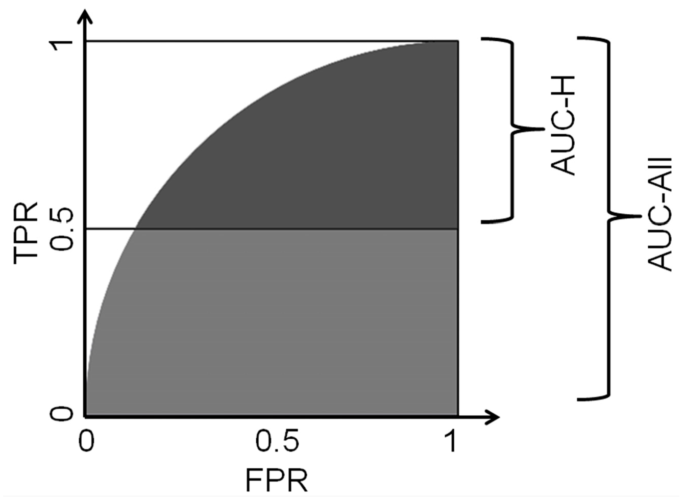
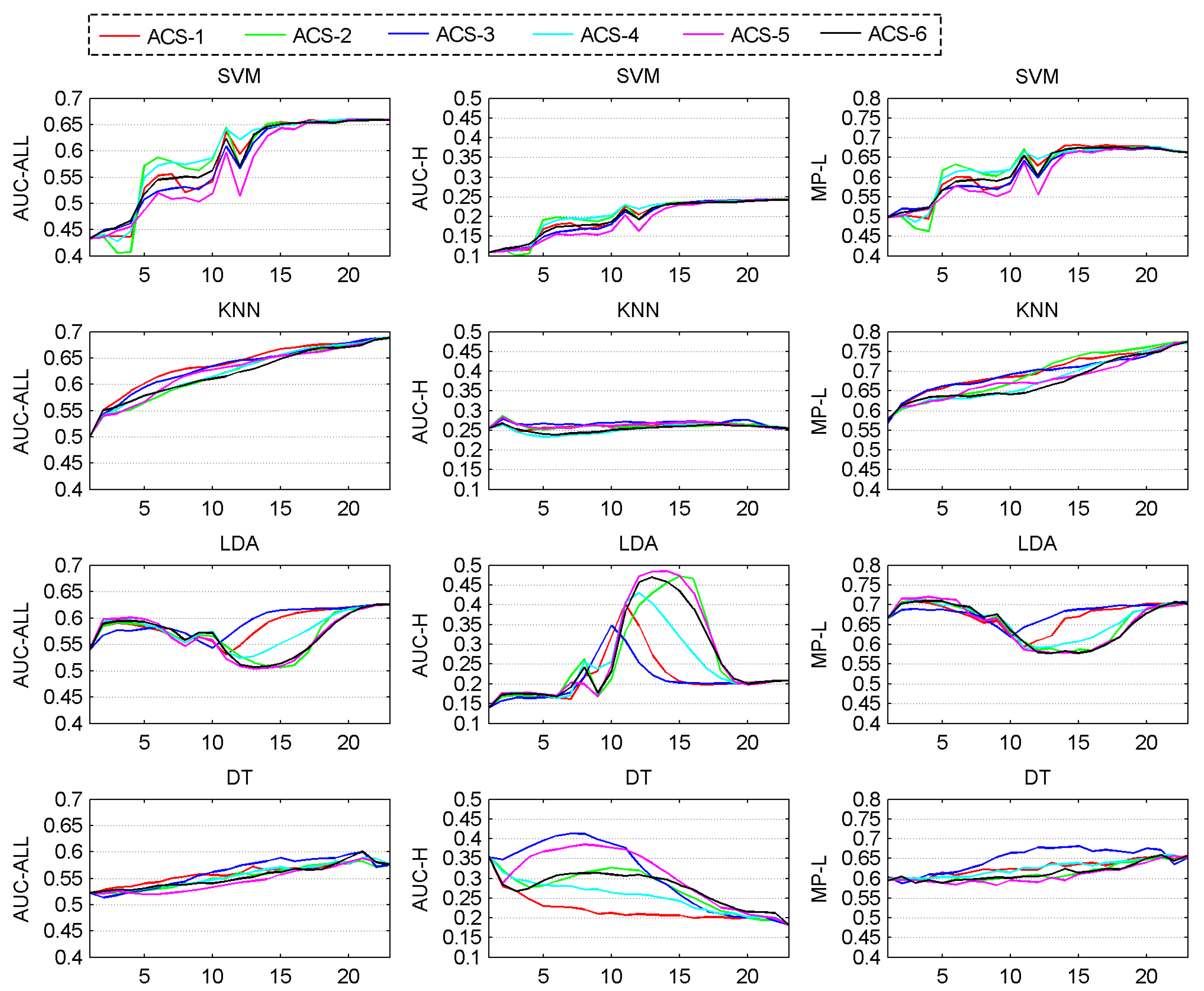
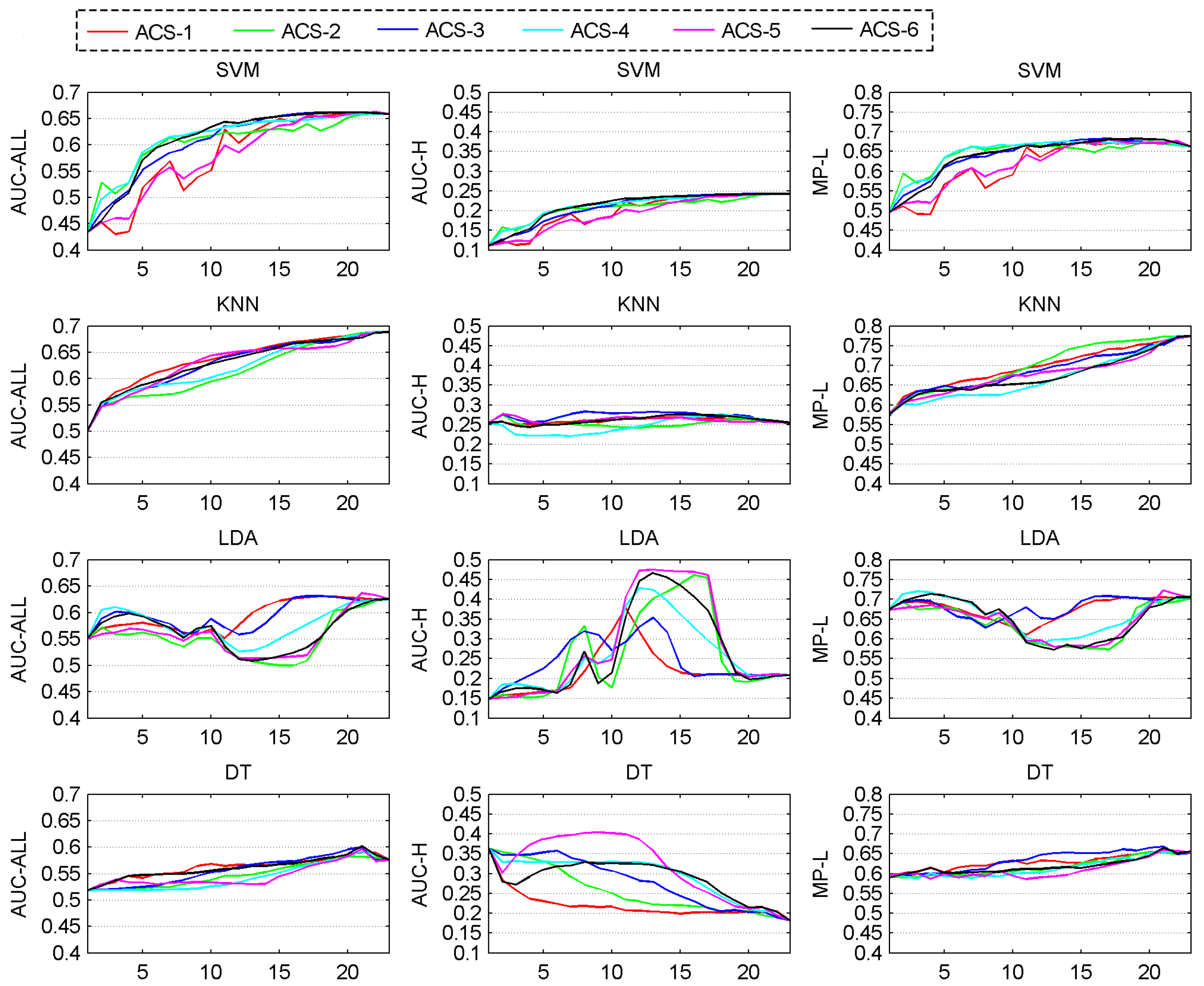
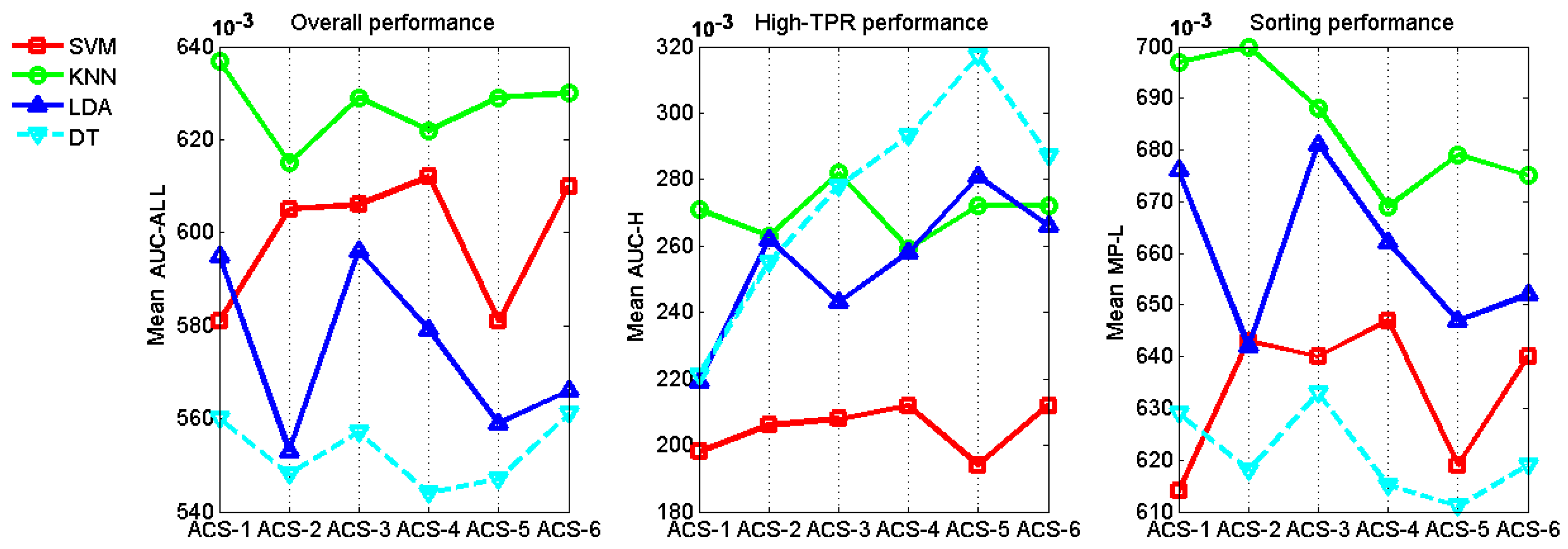
We want ACS methods to help a classifier improve its performance stably and as quickly as possible. Thus, the ideal curve of a classifier’s performance over iterations should be stably ascending, steep in the fore part and flat in the back part. Figure 5 shows the graphs of performance evolving over iterations of ACS methods coupled with SVM, KNN, LDA and DT classifier. By averaging the performance values of each curve in Figure 5, we get the mean performance values in Figure 6. The classifiers show different characteristics.

One observation is that in the case of high-PTR performance, KNN, LDA and DT which show bad (flat, unstable or descending) trends in Figure 5 have much better performance number in Figure 6 than SVM which shows good trend (stably ascending, steep in the fore part and flat in the back part) in curves. This might cause confusion when we choose a better classifier to work with ACS methods, because any variance of factors such as pre-processing, feature selection, parameter setting for classifiers, might dramatically change the mean performance value of a classifier and comparing classifiers in mean performance is very difficult to be on a fair base, we here suggest that more trust should be put on the trends of curves which more likely present the intrinsic features and less trust on the performance values that could be affected by too many factors. Based on this principle, Figure 5 shows five bad situations (KNN in high-PRT performance, LDA in all three kinds of performance and DT in high-PRT performance), in which ACS methods work badly and three good situations (SVM in all three kinds of performance), in which ACS methods work well.

KNN-based ACS methods show almost horizontal curves in the high-PTR performance, which means the increasing of training samples from any ACS method will not bring obvious improvement in high-PTR performance o KNN. DT-based ACS methods show almost descending curves in the high-PTR performance, which means the increasing of training samples causes the drop of performance. These phenomena might arise partly from the fact that the distributions of oil spill and look-alikes are heavily overlapping. When improving a system pursuing high-PTR performance, KNN and DT classifier should be considered carefully.

LDA-based ACS methods show dramatic fluctuations in their performance curves. LDA classifier takes the Gaussian assumption for the underlying distribution of oil spills and look-alikes. The big fluctuations means newly added samples change dramatically the shape of distributions learned previously. To deal with this problem, keeping a smooth change of distribution shape should also be considered in future when adding samples from ACS methods.

SVM-based ACS methods show good (stable and ascending, especially ascending quickly in the fore part and becoming flat in the back part of iterations) patterns in all three kinds of performance. That would be a merit when more than one services (each asks for a different performance) are demanded. In this case, only one (not the number of services) system needed to be built.

In the case of overall performance and sorting performance, randomly selecting samples (ACS-1) is always the best or second best when it is coupled with KNN, LDA or DT classifier, but not with SVM classifier. That may be because that KNN, LDA and DT are classifiers that try to make a decision based on some statistics from all samples in a certain region, while SVM makes the decision only on a few key samples (support vectors). Obviously, randomly selected samples (as from ACS-1) are more likely to maintain the statistics of the underlying distribution from which our training and test dataset come, but less likely to contain some key samples for SVM classifier.

The results in Figure 5 and Figure 6 also show that choosing a good ACS method for a specified classifier should be based on considering at least two important factors: the kind of performance chosen for optimization and the learning stages. A classifier may prefer different ACS methods in different performance measures. For example, the DT classifier favors ACS-1 in the overall performance and sorting performance but favors ACS-5 in the high-PTR performance. A classifier may also prefer different ACS methods in different stages of learning process. For example, SVM classifier favors ACS-2 and ACS-4 (methods that prefer choosing samples of more certainty) at the first half of the iterations in our study but ACS-5 and ACS-6 (methods that prefer choosing samples of more uncertainty and that choose samples half of more certainty and half of more uncertainty) at the second half.

3.2. Cost Reduction Using ACS Methods

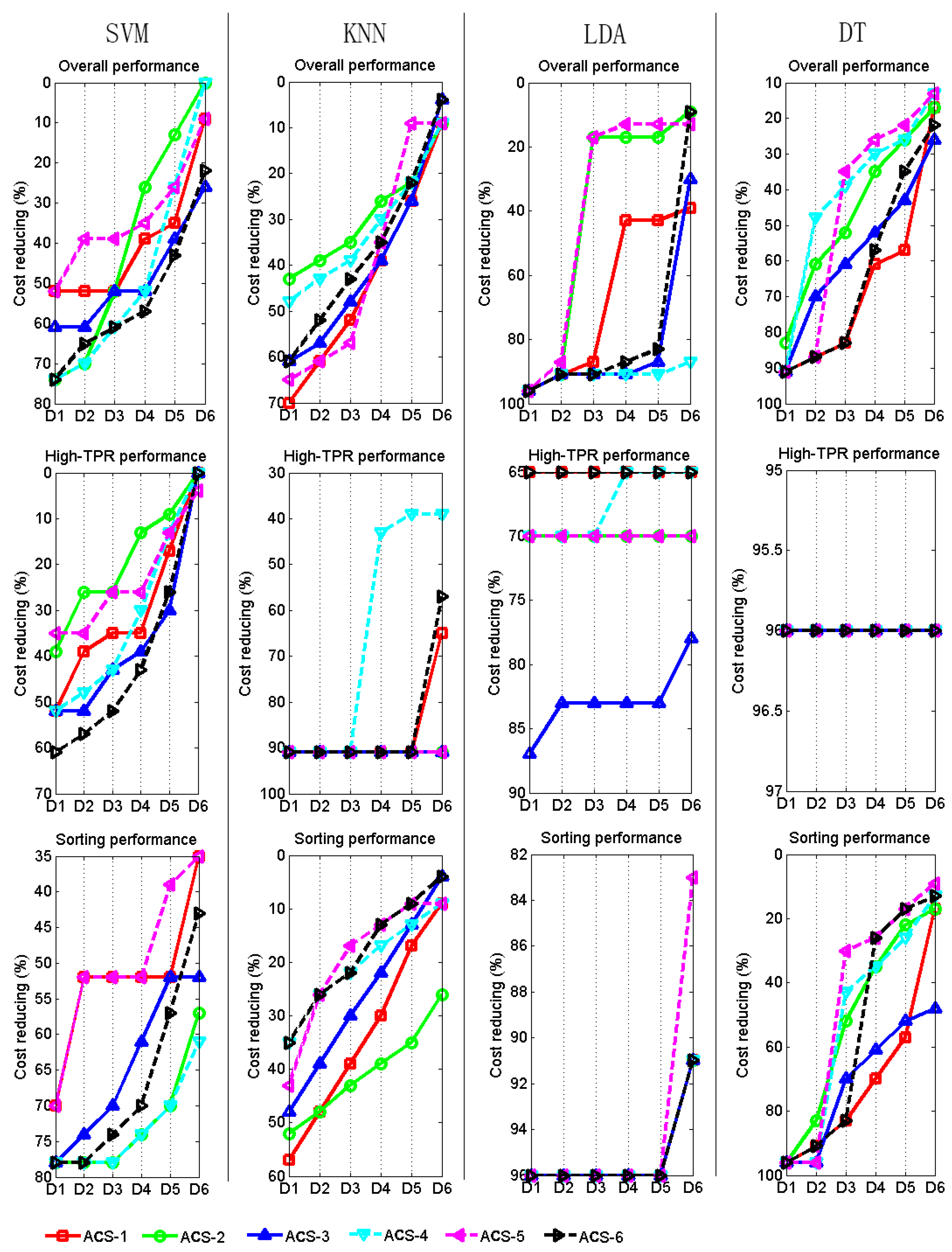
Figure 7 shows the cost reduction of using ACS methods to boost SVM, KNN, LDA and DT classifiers for achieving different destination performance. By selecting the maximum cost reduction for each classifier to achieve each destination performance, we obtain

Table 5. The maximum cost reduction of ACS methods for achieving designated performance D1 to D6 with SVM, KNN, LDA and DT classifiers. The numbers marked with gray show situations in which there are big cost reductions but ACS methods actually work poorly.

	Overall Performance (%)						High-TPR Performance (%)						Sorting Performance (%)
	D1	D2	D3	D4	D5	D6	D1	D2	D3	D4	D5	D6	D1	D2	D3	D4	D5	D6
SVM	74	70	61	57	43	26	61	57	52	43	30	4	78	78	78	74	70	61
KNN	70	61	57	39	26	9	91	91	91	91	91	91	57	48	43	39	35	26
LDA	96	91	91	91	91	87	87	83	83	83	83	78	96	96	96	96	96	91
DT	91	87	83	61	57	26	96	96	96	96	96	96	96	96	83	70	57	48

.

It should be noted that a big cost reduction in Figure 5 and Table 5 does not always means that ACS methods work successfully in that situation. The gray elements in Table 5 show five bad situations (also mentioned in Section 3.1), in which the cost reductions are very big but the ACS methods actually work so poorly that it is not necessary to analyze the cost reduction of these situations.

It can be seen that a considerable cost reduction can be achieved using ACS to boost classifiers. Taking the SVM, for instance, to get D5 destination performance, the maximum 43%, 30% and 70% reductions of cost can be obtained in overall performance, high-PTR performance and sorting performance, respectively. For D6 destination performance, the maximum 26%, 4% and 61% reductions of cost can be obtained in overall performance, high-PTR performance and sorting performance, respectively.

It can be seen in Figure 7 that, for SVM classifier, ACS-6 shows the best performance curve in overall performance and high-PTR performance, while ACS-2 and ACS-4 show the best curves in sorting performance. For DT classifier, ACS-1 works best in overall performance and sorting performance. For KNN classifier, ACS-1 work best in overall performance and ACS-2 works best in sorting performance.

There is still great potential to improve the cost reduction performance by improving the data preparation and tuning of classifiers, such as feature selecting, preprocessing, optimizing the parameters of model and using other definition of the informativeness preferred by the classifier.

Another method that may further improve the reduction of cost is to carry out the system serving and system training at the same time after the system has already had a sound performance. It can be seen in Table 5 that, using a sound designated performance (such as one of D1–D5), leads to a bigger cost reduction than selecting the perfect designated performance D6. Moreover, the income of service might cover the cost of continuing the system training once the system has been put into working.

3.3. Reducing Redundancy Amongst Samples (RRAS)

With SVM classifier, it can be seen in

Table 6. The difference of mean performance numbers between using and not using RRAS. The positive differences are marked with gray. A1 to A6 stand for ACS-1 to ACS-6.

	Overall Performance (10−3)						High-TPR Performance (10−3)						Sorting Performance (10−3)
	A1	A2	A3	A4	A5	A6	A1	A2	A3	A4	A5	A6	A1	A2	A3	A4	A5	A6
SVM	1.3	−17	−28	−19	−14	−26	0	−5	−14	−8	−6	−15	4.2	−22	−28	−23	−15	−22
KNN	0	5.9	2.1	1.8	−5	−9	1.1	8.3	−3	5.3	1.7	−7	1.5	−6	6.8	10	1	1
LDA	−7	15	−4	−2	6.3	1.8	−1	0	−34	−15	−12	−3	−2	14	−1	1	6.6	2
DT	−3	4.4	5	11	0	−7	0.7	17	29	−39	−12	−11	−1	−3	14	11	−2.2	−4

that RRAS reduces the mean performance of most ACS methods except ACS-1. Because the key samples (support vectors) only exist in a relatively small region near the decision boundary for SVM classifier, increasing the diversity of samples by RRAS would not help choose samples from the key region, which is very small compared with the whole feature space. Compared to not using RRBS (Figure 5), performance fluctuations in Figure 8 are increased at the former part of iterations and weakened at the end part of iterations, and ACS-2, ACS-4 change from the first and second best methods to the first and second worst at the first few iterations of all graphs. These phenomena could also be caused by the increased randomness of selected samples by RRAS. It seems that RRAS is not suitable for SVM-based ACS methods in our case.

For KNN classifier, the RRAS does not bring significant improvement in the shape of curves in Figure 8 compared to curves in Figure 5, but does slightly increase the mean performance values of more than half of ACS methods (see Table 6). For KNN classifier, the more thorough the training sample dataset can represent the true underlying distribution, the higher performance it can obtain. The RRAS can improve the representative ability of selected samples by first grouping all samples into clusters and then selecting one from each cluster as the representative sample and therefore seems suitable for some KNN-based ACS methods.

In Table 6, there are some performance improvements and drops for ACS methods with LDA and DT classifier, but it is hard to analyze the reasons.

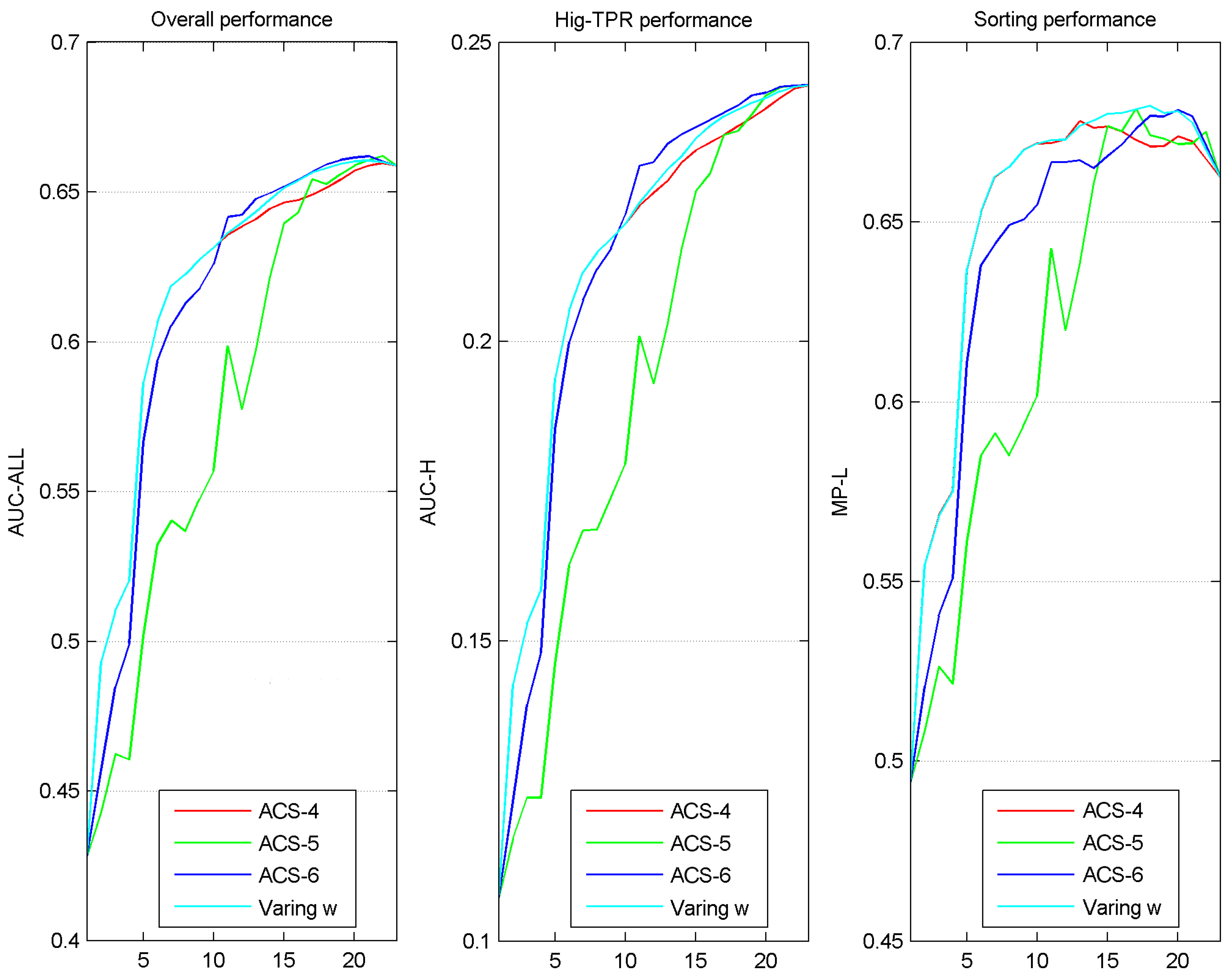
3.4. Adjusting Sample Preference in Iterations

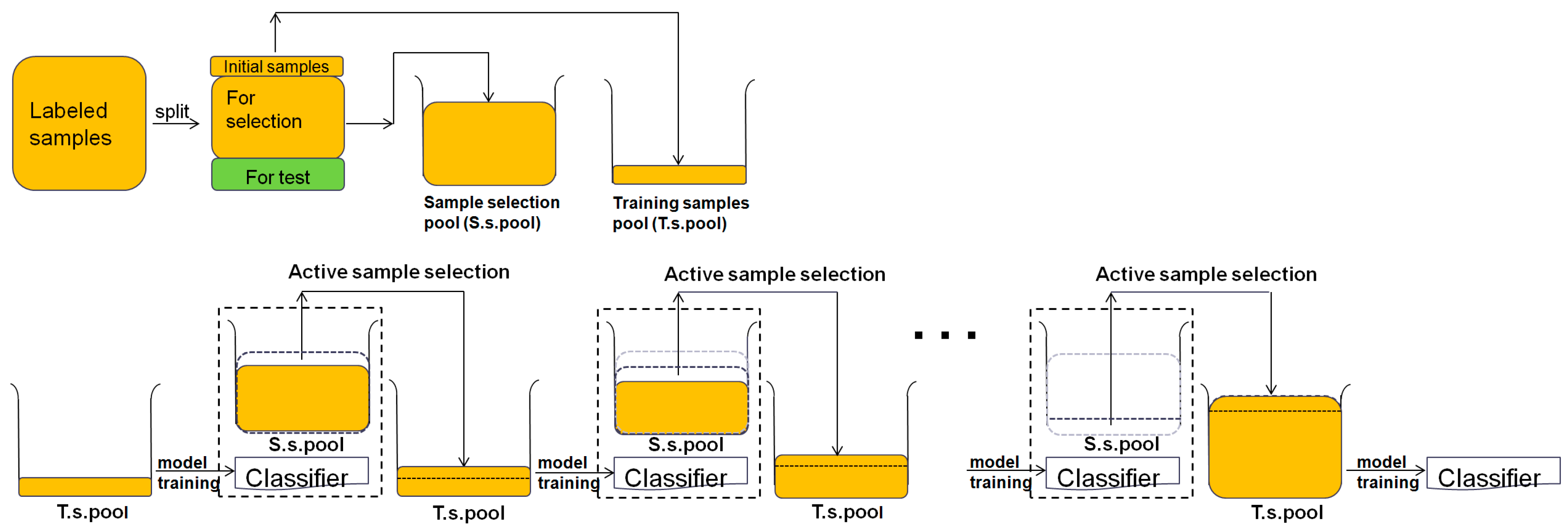
Figure 9 shows the performance-evolution graph of the ACS method with varying parameter for sample selection, coupled with SVM. It can be seen that the ACS method with parameter w varying according to Function (1), at most iterations, matches or outperforms any of the other fixed-w methods (ACS-4 is with w = 1, ACS-5 with w = 0, and ACS-6 with w = 0.5). Here, we set the parameters of Function (1) as a = 20, b = 0.5, c = 0.5. The varying-w method obtained mean performance values (by averaging performance numbers on its curves in Figure 9) 0.614, 0.213 and 0.650 for overall performance, high-TPR performance and sorting performance, respectively. These mean values are all better than the best ones of SVM classifier in Figure 6, i.e., 0.612, 0.212 and 0.647.

Although adjusting parameter w in an iteration-based manner seems to be a good strategy for improving system performance in our study, the use of such a strategy must have a theoretical or empirical basis. Otherwise, there is no guarantee that such good results might also be achieved in other datasets. Although the exploration-and-exploitation criterion [59] is a commonly accepted one (our method here is derived from it), it is only suitable for SVM classifier in this study. The unsuitability for KNN, LDA and DT classifier can be seen clearly in Figure 5, in which, when coupled with these classifiers, ACS methods preferring samples of certainty does not perform well at the former part of iterations and so do the ACS methods preferring samples of uncertainty at the end part. Criteria similar to exploration-and-exploitation suitable for SVM need to be found and verified for other classifiers in the future.

4. Conclusions

In this study based on a ten-year RADARSAT dataset covering west and east coasts of Canada, AL has shown its great potential of training sample reduction (for example, a 4% to 78% reduction on training samples can be achieved in different settings when using AL to boost SVM classifier) in constructing oil spill classifiers. That means the real-world projects of constructing oil spill classification systems (especially when it is hard to accumulate a large number of training samples, such as when supervising new water area) or improving existed systems may benefit from using AL methods. In the cases where AL are used for classifier training, we boldly suggest that the expensive, time-sensitive, and difficult field verification work should be conduct only for those targets that are identified by AL as the “important” targets to significantly improve the classifier training efficiency. AL could reduce training data, whether they are obtained by expert-labeling or by field-verifying. Generally, field-verified data are better than expert-labeled data for training due to the higher verification accuracy of the field investigation approach. Nevertheless, when it is hard or impossible to do fieldwork, asking experts for labeling is also acceptable. Both labeling approaches benefit from the efficient learning process of the AL method for classifier construction.

Our study shows that not all classifiers can benefit from using AL methods according to all measures. In some cases (in this paper, KNN in high-PRT measure, LDA in all three kinds of performance measures and DT in high-PRT measure), the AL methods may not help improve performance, or even reduce it.

Of the four classifiers tested in this paper, the SVM is the best for using AL methods for the following reasons. First, it can benefit greatly from some basic ACS methods (in our case, ACS-2, ACS-4 and ACS-6), showing perfect performance evolving curves with steeply ascending fore parts and flat back parts. Second, the good ACS methods for SVM in one kind of performance measure will also be good in other kinds of performance measures. That would be a merit when more than one services asking for different kinds of performance are demanded. In this case, only one system needed to be built and that surely will greatly reduce costs. Third, its performance could be further improved by ACS method using exploration-and-exploitation criterion, which considers different sample preference in different learning stages.

The exploration-and-exploitation criterion is suitable for SVM but not for KNN, LDA and DT classifiers. The criteria considering different sample preference in different learning stages and being suitable for other classifiers may also exist and should be found and studied in the future.

The thorough knowledge of a classifier’s preference on training samples is the key to achieve efficient AL-based classification system, because all AL operations, such as choosing AL strategy and ACS methods, adjusting sample selection preference in iterations, depend on knowing a classifier’s sample favoritism to identify the best samples that satisfy the demands of the classifier. Thus, further study should also focus on investigating the sample preference mechanism of a classifier to build a high-performance AL-based frame on it.