Ship-Iceberg Discrimination in Sentinel-2 Multispectral Imagery by Supervised Classification

Abstract

The European Space Agency Sentinel-2 satellites provide multispectral images with pixel sizes down to 10 m. This high resolution allows for fast and frequent detection, classification and discrimination of various objects in the sea, which is relevant in general and specifically for the vast Arctic environment. We analyze several sets of multispectral image data from Denmark and Greenland fall and winter, and describe a supervised search and classification algorithm based on physical parameters that successfully finds and classifies all objects in the sea with reflectance above a threshold. It discriminates between objects like ships, islands, wakes, and icebergs, ice floes, and clouds with accuracy better than 90%. Pan-sharpening the infrared bands leads to classification and discrimination of ice floes and clouds better than 95%. For complex images with abundant ice floes or clouds, however, the false alarm rate dominates for small non-sailing boats.

1. Introduction

Marine surveillance and situation awareness is essential for monitoring and controlling piracy, smuggling, fishing, irregular migration, trespassing, spying, traffic safety, icebergs, sea ice, shipwrecks, the environment (oil spill or pollution), etc. Black ships are non-cooperative ships with non-functioning transponder systems. Their transmission may be jammed, spoofed, sometimes experience erroneous returns, or are simply turned off deliberately or by accident. Furthermore, AIS satellite coverage at high latitudes is sparse, which means that other non-cooperative surveillance systems, including satellite or airborne systems, are required.

The Sentinel satellites under the Copernicus program [1] provide excellent and freely available multispectral imagery with resolutions down to 10 m in four bands, and Synthetic Aperture Radar primarily with resolution down to 90 m in the high resolution extra wide swath ground range detection mode. Their frequent transits over the polar regions make these satellites particularly useful for Artic surveillance and for monitoring icebergs, sea-ice coverage [2,3], ships [4,5,6,7,8,9,10,11,12,13,14,15,16,17], oil spills [18,19,20], crop and forestation [21,22].

The orbital period is 10 days for the Sentinel-2 (S2) satellites A + B, each of which carries multispectral imaging (MSI) instruments. The image strips overlap at a given point on the Earth, and the typical revisit period for each satellite is two or three days in Europe and almost daily in the Arctic. S2 MSI has the potential to greatly improve the marine situational awareness, especially for non-cooperative ships—weather permitting.

The Iceberg Alley [3] is a dangerous iceberg infested route running from west Greenland and Baffin Island and Newfoundland, down into a strait where many ships, including the Titanic, transit the North Atlantic. In September 2016, Crystal Serenity was the first cruise ship that risked sailing from Alaska to Greenland through the Northwest Passage, which is infested with uncharted reefs, sea ice and huge icebergs. Since satellite AIS coverage is very limited at these latitudes, ships are essentially non-cooperative in the Arctic.

SAR imagery [2,3,4,5,6] is weather independent, but generally has lower resolution, is subject to speckle noise, motion blurring, and has target and angle dependent reflection coefficients. SAR is therefore less useful for small ship detection and classification. In addition, SAR is unable to detect objects with low dielectric coefficients as wooden or glass fiber boats. The high resolution S2 MSI can, as is shown below, improve the classification, discrimination and multispectral identification of ships and threats from icebergs, unless clouds cover the sea.

This article focuses on search, classification and discrimination of ships, islands, icebergs, sea ice, wakes and clouds in S2 MSI. For this reason, two regions of interest have been selected: Skagen on the northernmost tip of Denmark, where there are often a large number of ships, boats, wakes and clouds, and Nuuk the capital of Greenland where there are numerous fishing boats, icebergs and ice floes. The classification method is based on elements of principal component analyses (PCA) and also k-method algorithms [23]. The analysis identifies the most useful aspects of these methods, and provides a direct physical understanding and classification of the objects to be found and discriminated in Arctic and other environments. Based on this analysis, a supervised classification algorithm is developed that exploits both the spatial and spectral information in the multispectral images from S2 MSI.

Detection is relatively easy due to the high sensitivity and dynamic range of the images, and the generally dark sea background. Recognition is based on high-resolution images that allow for an accurate and robust classification of objects from the spatial and spectral information. The accuracy and confidence of all of this is fundamentally reliant on the target’s spectral reflectances and size. The analysis and discussion of the accuracy of the recognition and identification, based on a target’s S2 MSI data, are obtained as outputs from the S2 MSI detection, recognition and identification process.

The paper is organized such that the S2 data are described first, followed by a description of the data analysis. Subsequently, the classification model is described based on spatial and spectral characteristic of the objects, followed by a presentation of the results for classification of ships, islands, icebergs, grey ice, wakes, etc. including a discussion of the confusion matrix and false alarms. Finally, a summary and outlook are also offered.

2. Satellite Images and Method of Analysis

The S2 multispectral images are analyzed by using dedicated software developed for the purpose of small object classification in large images in several multispectral bands with different pixel resolutions. The images have been preprocessed by the sen2cor algorithm for atmospheric corrections [24]. The processing is mainly designed for object search and classification, and is fast (a few seconds) depending on the size and complexity of the mega- to giga-pixel images with 4048 (12 bit) grey levels. We will describe in detail how the segments are detected, and how their multispectral reflectances and several spatial properties are calculated.

Subsequently, we describe a supervised classification of the segments as objects based on both spatial and spectral properties that are related to physical properties of the objects. The classification is based on—but not restricted to—standard methods from principal components analysis (PCA), k-means and Mahalonobis distances [23], but is tailored specifically to optimize the classification of smaller ships and icebergs. The success of the classification method lies in choosing the best classifiers and thresholds that correctly identify most segments.

2.1. Sentinel-2 Multispectral Images

S2 carries the wide-swath, high-resolution, multispectral imager (MSI) with 13 spectral bands with 10, 20 or 60 m resolution [1]. As we are interested in detailed small object classification and discrimination, we will focus on analyzing the four bands with 10 m resolution, namely B2 (blue), B3 (green), B4 (red) and B8 (near-infrared). In addition, the two short wave infrared bands B11 and B12 with 20 m resolution are pan-sharpened and included.

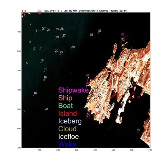
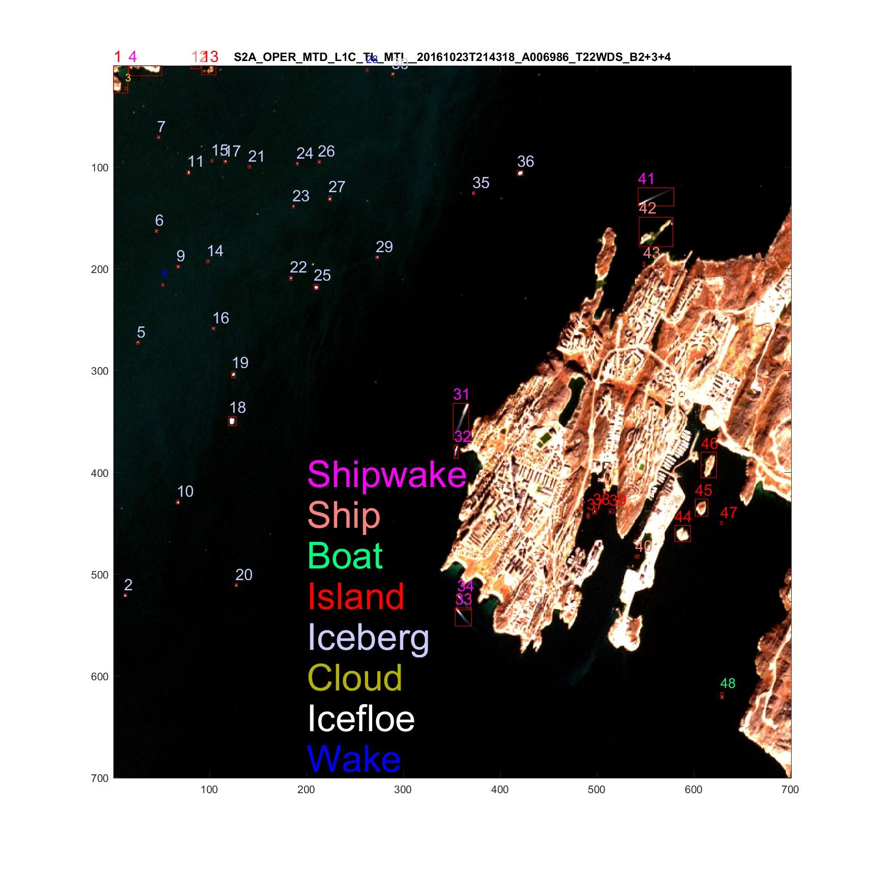
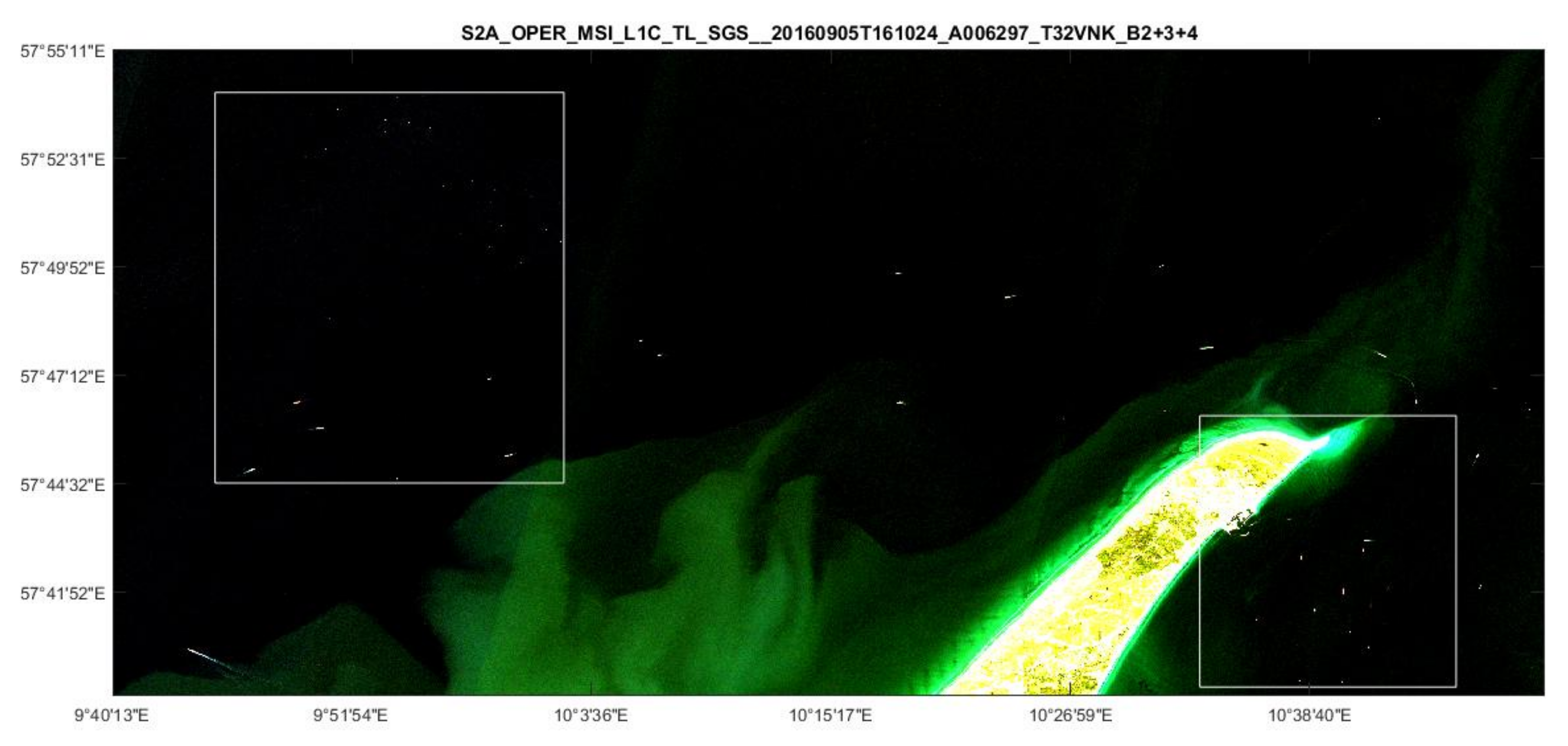
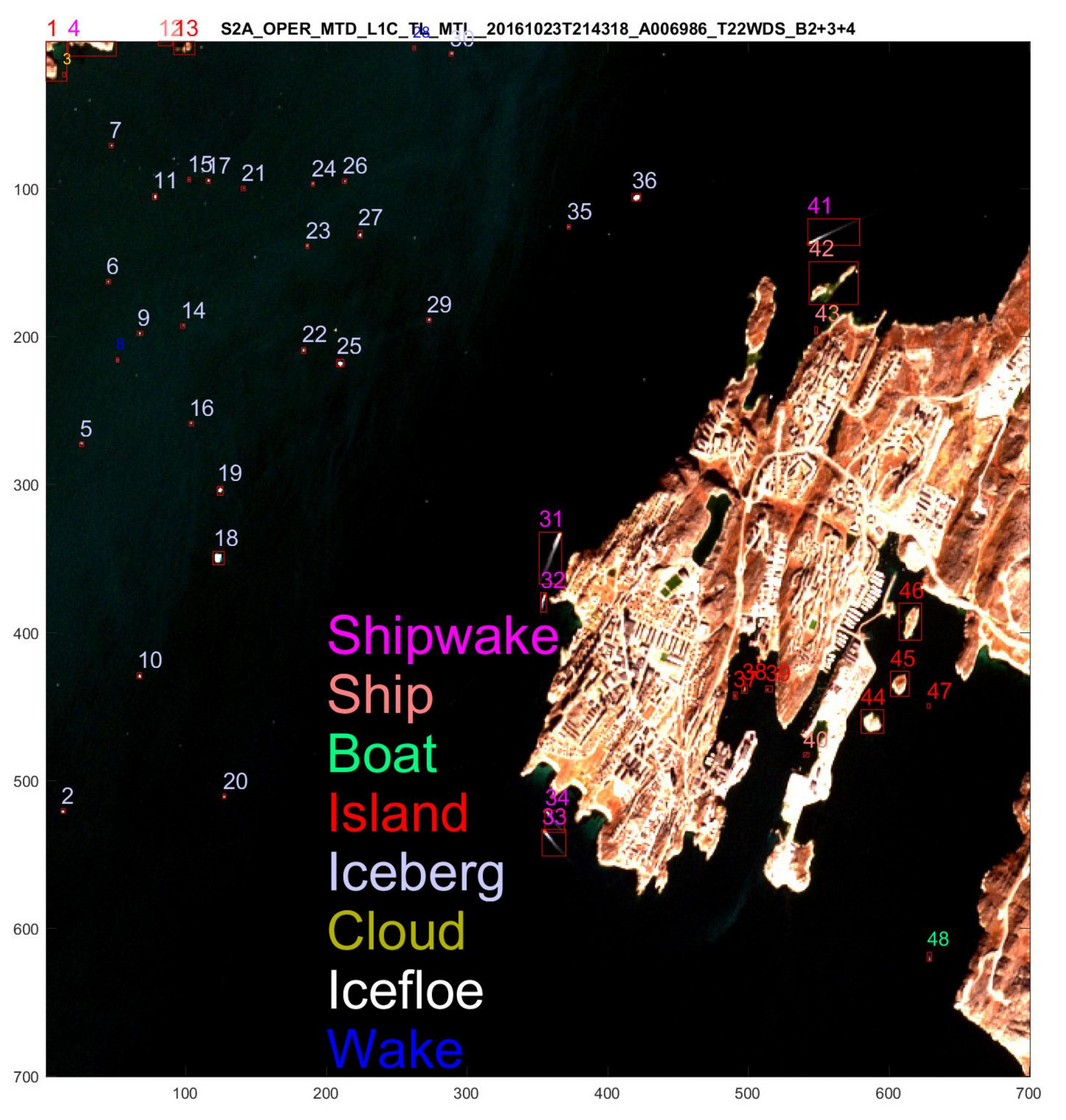
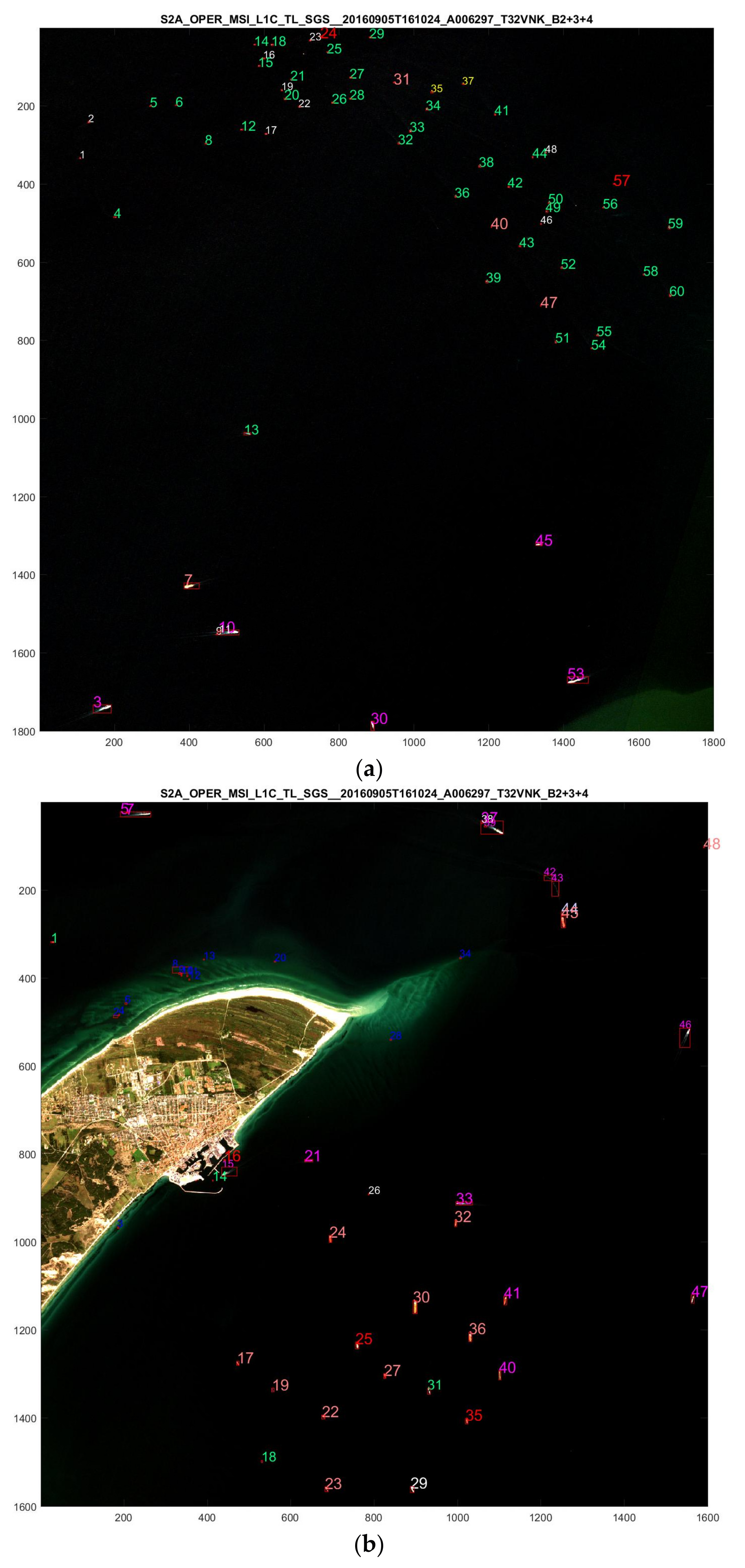
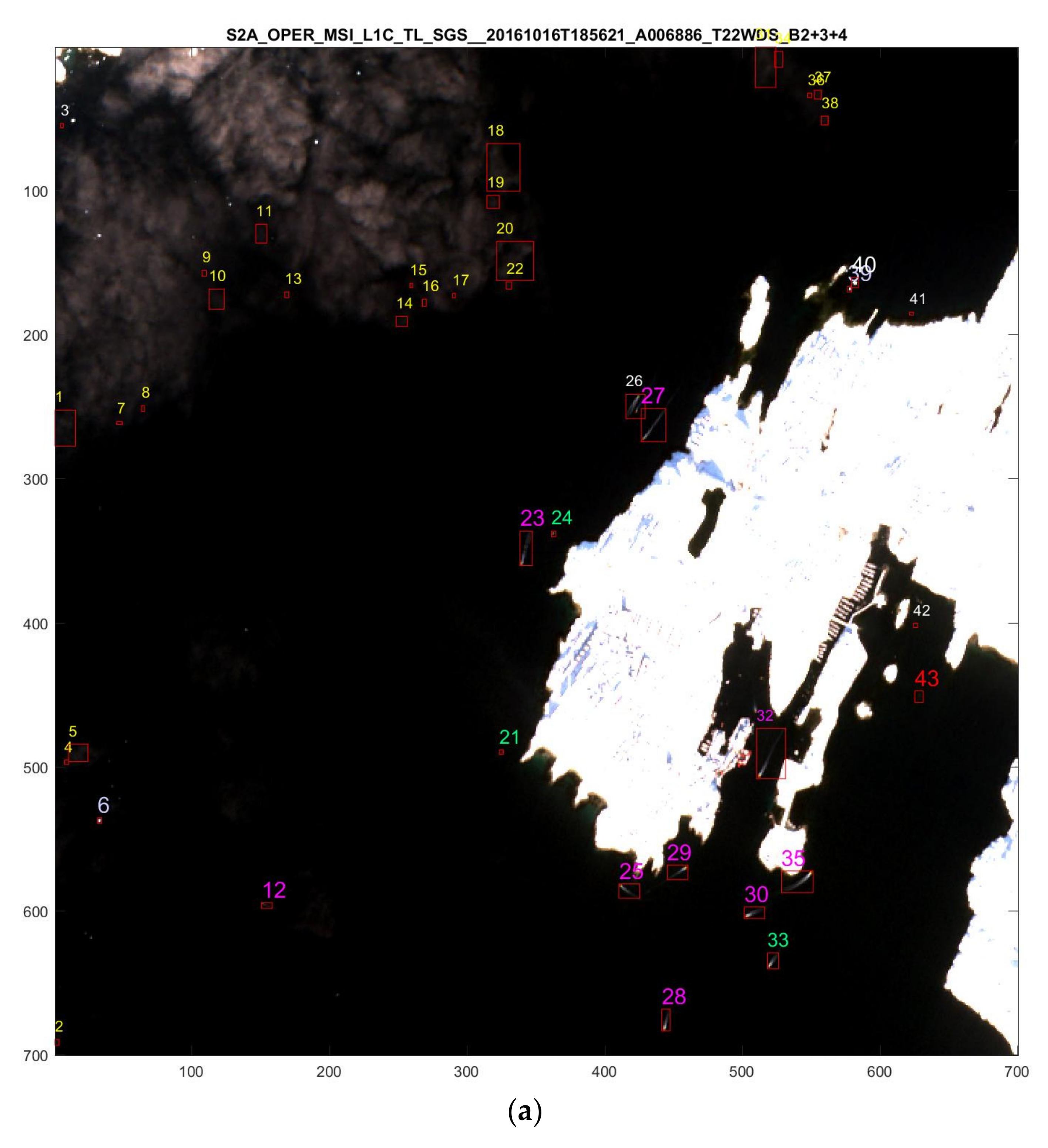
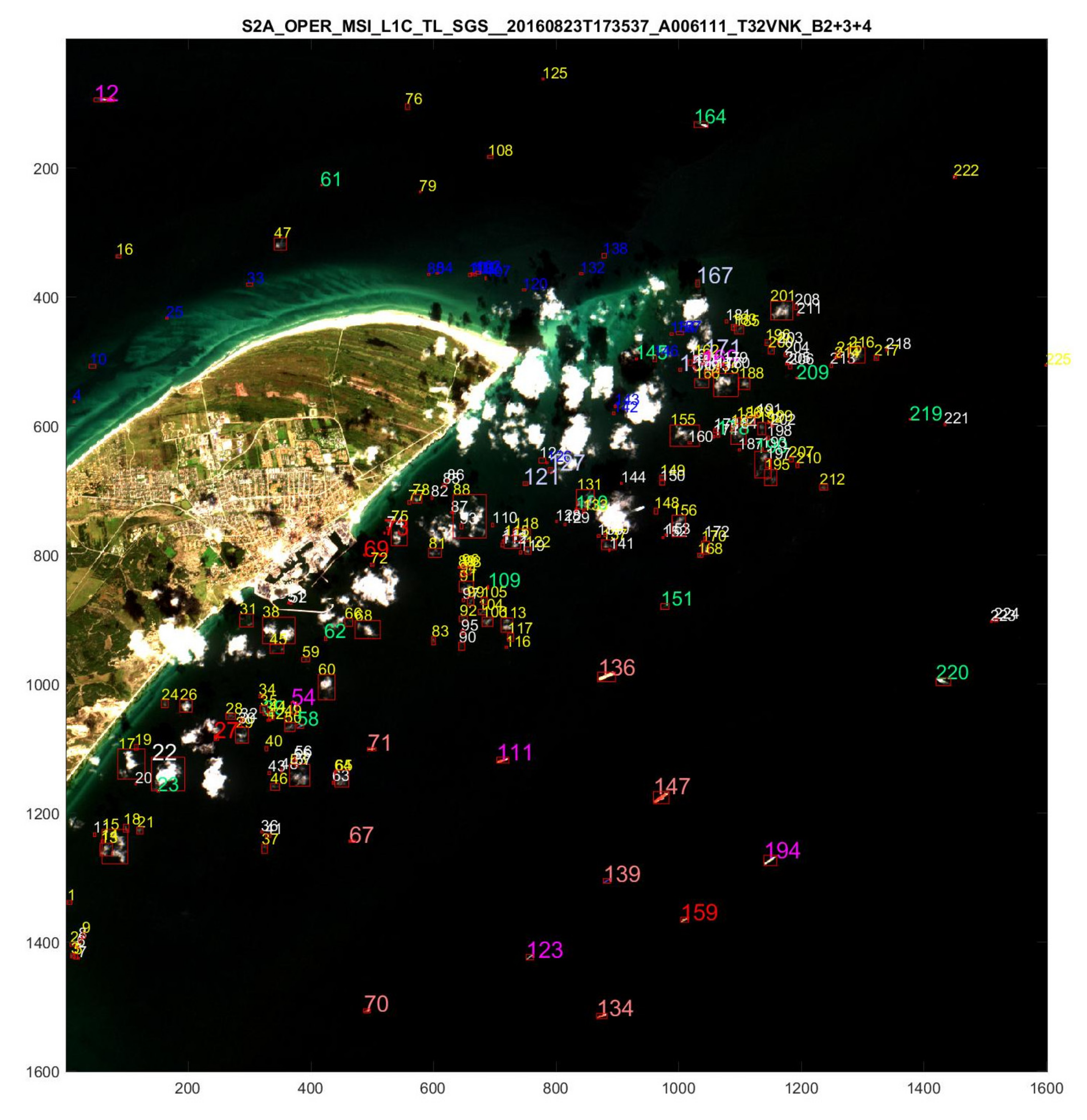
Two regions of interest are selected: Skagen, the northernmost tip of Denmark (Figure 1), and Nuuk, the capital of Greenland (Figure 2). These images are convenient for classification because the objects are relatively easy to identify as there is only ice and a few islands and sailing fishing boats in Nuuk. In contrast, a number of large ships, smaller boats, wakes and clouds are present at Skagen. 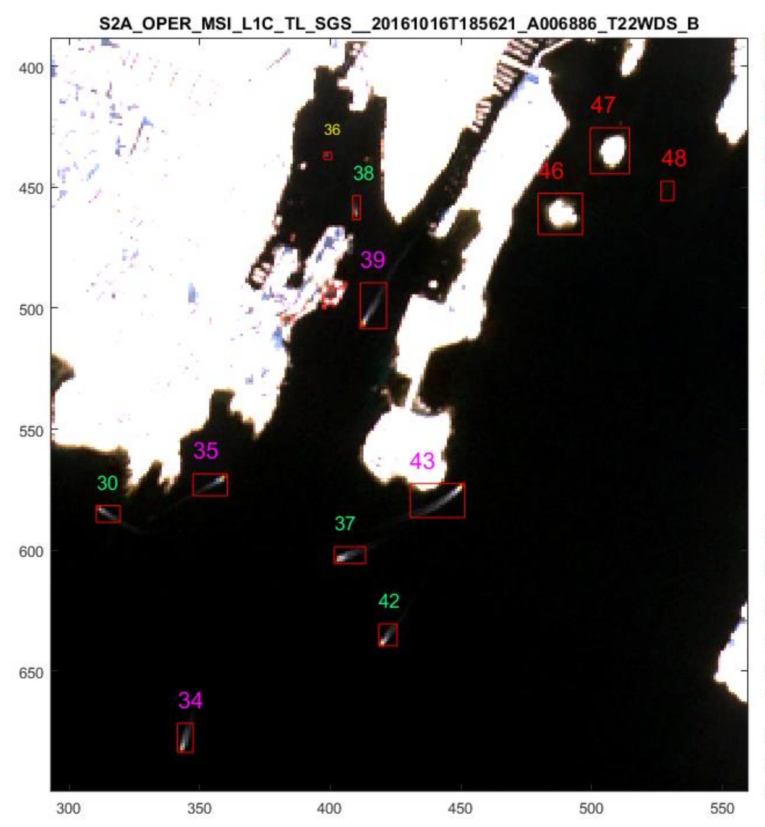The S2 images analyzed here are recorded over Skagen on 23 August 2016 shown in Figure 1 (with analyses in Figure 3, Figure 4, Figure 5 and Figure 6) and excerpts of Figure 1 in Figure 7a,b. The S2 images over Nuuk are from 23 September (Figure 2), 16 October (Figure 8a) and 23 October (Figure 8b with analysis in Figure 9), all in 2016. Nuuk is situated on 64° north latitude just below the polar circle. S2 passes over Nuuk around noon, therefore there is always light all year around, although shadows can be long during winter. S2 data over Nuuk are processed and made available with a few days interval except in December and January. Finally in Figure 10 we return to a cloudy image over Skagen from 1 September 2016.

The images contain reflectances I_Bx(i,j) for each of the 13 multispectral bands x = 1, …, 8, 8A, 9, 10, 11, 12. The pixel coordinates (i,j) are the (x,y) coordinates in units of the pixel resolution l, which is l = 10 m for the blue, green, red and near-infrared bands B2, B3, B4, and B8, respectively; l = 20 m for B5, B6, B7, B8A, B11, and B12; and l = 60 m for B1, B9, and B10.

To detect an object, its reflectance must deviate from the sea background in one or more spectral bands. Most objects we have encountered reflect more light in all bands than the sea and we therefore subtract the sea background in all spectral bands. For resolving the objects optimally, we sum the reflectances in the four high-resolution bands B2 + B3 + B4 + B8 with sea background subtracted

$${\mathrm{I}}_4\left(i,j\right) = {\mathrm{I}}_{\mathrm{B}2}\left(i,j\right)+{\mathrm{I}}_{\mathrm{B}3}\left(i,j\right) + {\mathrm{I}}_{\mathrm{B}4}\left(i,j\right) +{\mathrm{I}}_{\mathrm{B}8}\left(i,j\right)-\mathrm{background}.$$

(1)

Since the sea covered substantially more than half of the area in all our images, the median reflectance value for each images provided an accurate and robust value for the background. This total reflectance image I₄ has the highest resolution and contrast to the sea and is therefore optimal for object search and detection.

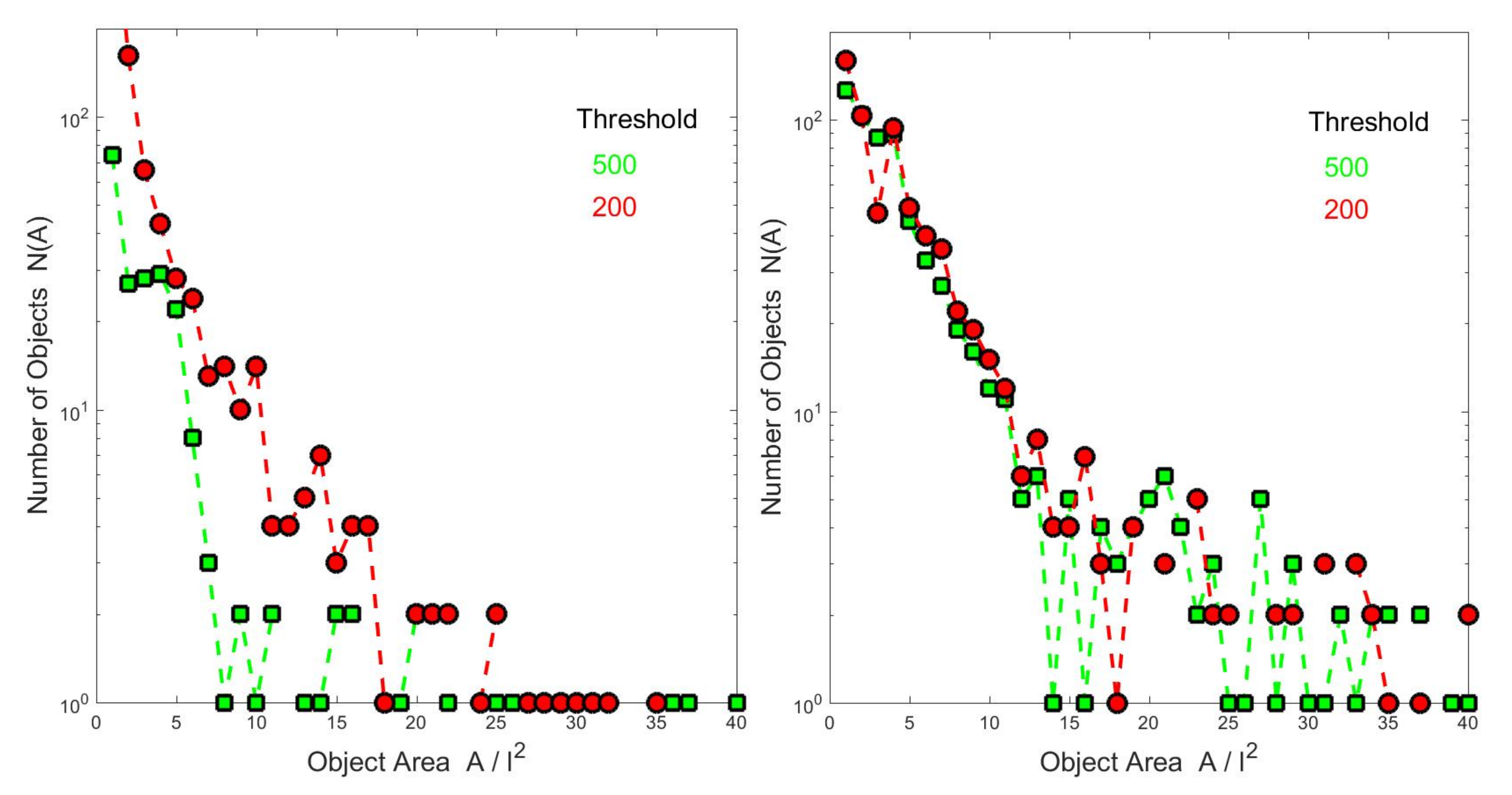
To be seen, the object must exceed a threshold which depends on the scenario. Examples of the threshold dependence are shown in Figure 3 and discussed in the following subsection. In normal sea background, the threshold can be chosen rather low, whereas in icy Arctic oceans with widespread ice floes or images with clouds, it may be advantageous to choose a higher threshold in order to distinguish objects from ice floes and clouds. Thereby the false alarm rate for ship detection is much reduced as the large number ice floes with high spatial and spectral variation is suppressed. However, as a result, we risk that, e.g., small and slow ships are “hidden” in a background of ice floes, as will be discussed later.

2.2. Spatial Classification of Segments as Objects

Treating the total reflectance image I₄(i,j) as a matrix, we construct a connectivity matrix in which the matrix pixels with reflectances above the threshold T are assigned 1 and those below 0. In this connectivity matrix, all neighboring entries with value 1 are then connected as a segment (s), and listed s = 1, N_s, where N_s is the total number of separate segments found in the image. Each segment has an observed area corresponding to the sum over the pixels in the segment

$$\mathrm{A}\left(\mathrm{s}\right)=l^2{\displaystyle \sum }_{i,j \in s}^{I_4\left(i,j\right) > \mathrm{T}}1$$

(2)

We refer to Refs. [21,22,23,24] for other segmentation methods.

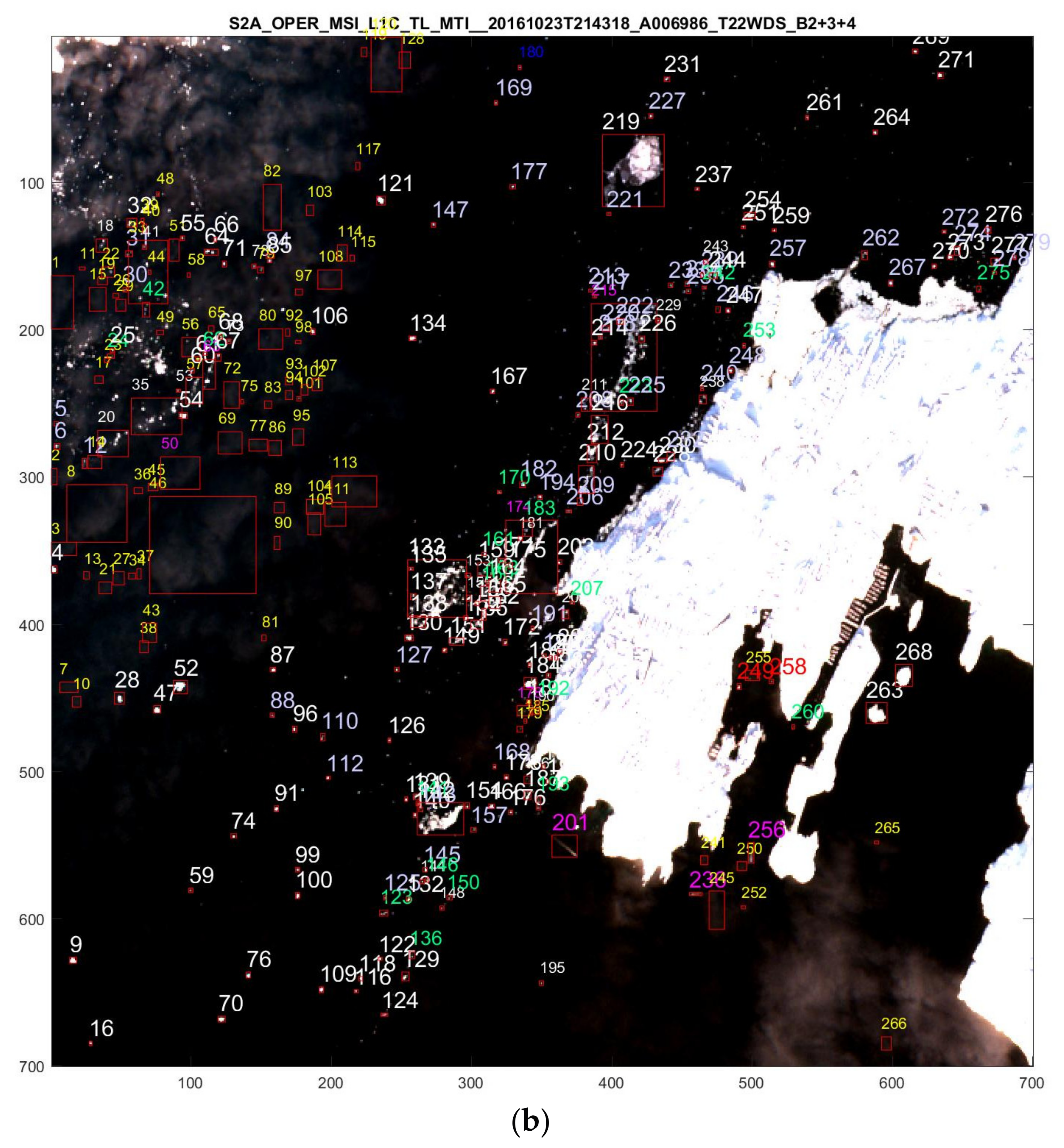
The number of segments vs. area, which is the same as the number of objects vs. area, is shown in Figure 3 for the satellite images of Figure 1 and Figure 8b for two different thresholds. Both thresholds are low compared to the up to 4 × 4048 grey levels minus background. The lower threshold is used in all figures except Figure 8a,b, where the higher threshold is employed. In both cases, the number of small objects decrease for the higher threshold as could be expected. The number of objects drop almost exponentially from hundreds of small objects to very few or none large objects. We find that, for the medium and large size objects of interest in this work, the detection and number is rather robust although their area may decrease slightly with increasing threshold.

The classification scheme will later identify the segment as an object, e.g., a ship, island, iceberg, ice floe, wake or cloud. Segments are pixel based, whereas object classification is based on a priori knowledge or inspection.

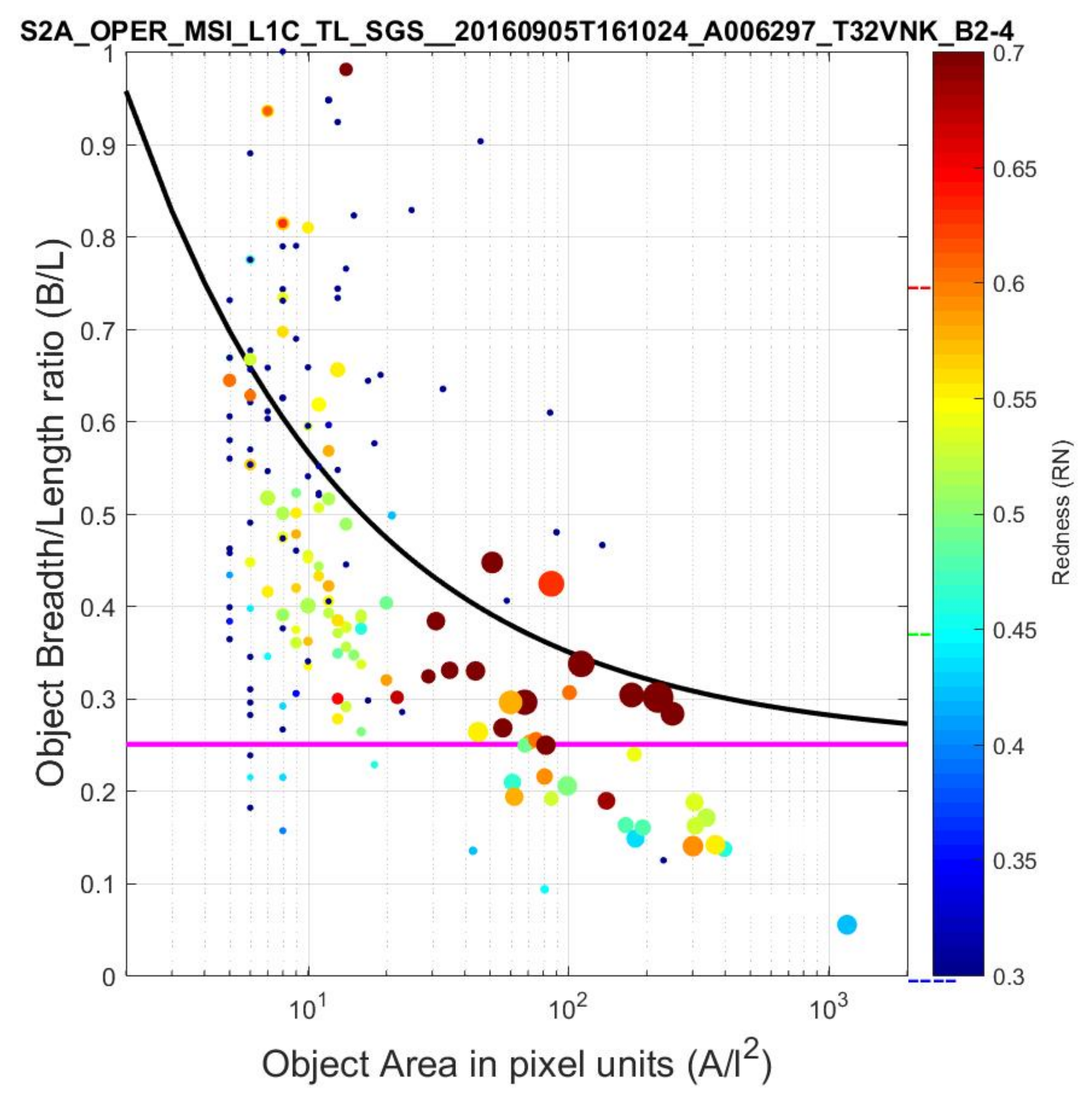
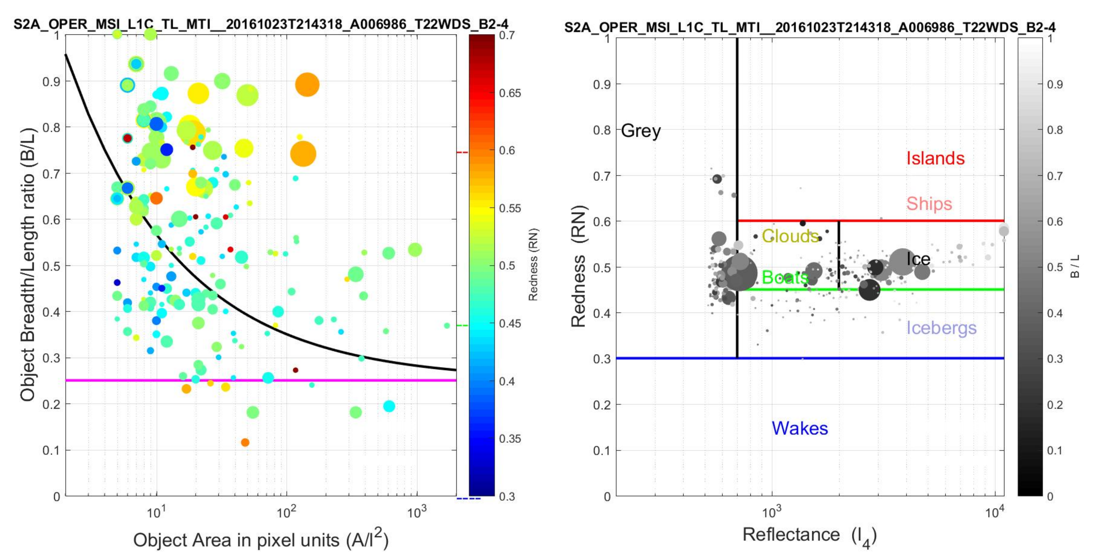
As described in Ref. [13], one can calculate the center of mass coordinates, length (L), width or breadth (B), orientation angle, eccentricity $ϵ = \sqrt{1-{\mathrm{B}}^2/{\mathrm{L}}^2}$, convex area, circumference as well as a number of other spatial parameters for the segment. These parameters are exploited for spatial classification of the segments as objects. For example, ships are elongated and generally have small B/L, and ships sailing at high speed create a long wake resulting in a very small B/L. This is observed in Figure 4, where a scatter plot of B/L vs. observed area A is shown for all objects in Figure 1. The ships tend to cluster at low B/L or small A. The reason for this is that smaller boats may have breadths of order the pixel resolution l = 10 m or less, but usually appear at least two pixels wide, and they therefore appear to be less elongated than they actually are physically. If we add a pixel length l to each side of the true ship breadth B₀ and length L₀, the observed area is A = (B₀ + 2l)(L₀ + 2l), and the observed ratio of the breadth to width is approximately

$$\frac{B}{L}\cong \frac{B_0+2l}{L_0+2l}\cong r+2l\sqrt{\frac{r}{\mathrm{A}}},$$

(3)

where r = B₀/L₀ is the true ship breadth to length ratio. As described in Ref. [13], this ratio is typically r ≅ 0.15 for most large ships, but for smaller boats filling a few pixels it can vary around this value. We therefore choose a larger value r = 0.25 to assure that most ships and small boats are captured. As result, we get fewer false negatives but at the cost of some more false positives. The ratio is shown with black curve in Figure 4, and defines the spatial classification of ships and boats below the curve and islands, icebergs and other objects above. In the following we shall classify elongated segments as having B/L less than the criterion of Equation (3) with r = 0.25, also shown by the black curve in Figure 4.

The convex area of the segment provides additional spatial information. For example, the moon near new moon has a curved concave side. Its convex area is defined as the connected area which is the half moon, and which is larger than the solar reflective surface area. Between half and full moon, however, the convex area is the same as the reflective area. Likewise, a ship with or without wake is rectangular and straight, and therefore its area and convex area are almost the same. Islands and ice floes often curve or vary in width resulting in a convex areas larger than their observed area. We can therefore make use of the condition that boats should have a ratio of convex area to observed area less than 1.3, found by minimizing the number of confusions, whereby we optimize the discrimination of ice floes from ships.

The segment circumference also provides information on the regularity of the segment, and one can define the compactness as the ratio of the circumference to area [9]. The limited pixel resolution does, however, not resolve object borders well, and we do not find this parameter useful for classifying smaller objects.

In a more general principal component analysis of the 2D images (2DPCA), a number of eigenvectors and eigenvalues are calculated for the object. For example, a ship, the two principal spatial eigenvectors are the symmetry axes along and transversely to the ship axis, and the corresponding two eigenvalues are proportional to the ship length and breadth [13]. 2DPCA is useful for identifying the parameters that vary the most, but these are not necessarily the best for discrimination. In addition, it can be cumbersome to interpret the eigenvalues correctly in terms of physical parameters and for classification. We therefore use the principal components only as a guideline for selecting the physical parameters most useful for classification.

A very useful classification method is k-means clustering or k-nearest neighbor, where k objects are assigned a number of classifiers [23]. For example, a ship should have small B/L and area A smaller than ca. 300 pixels (30,000 m²) but convex area not much larger than its area, as well as spectral properties discussed below. A segment is classified to that object which deviates least from its classifiers, i.e., the object that the segment resembles the most. Least deviation can be defined in a number of ways, e.g., as a weighted least mean square value. We shall employ a more direct and sharp classification algorithm that for each classifier checks whether it is above or below a threshold. This threshold is a physical parameter that is determined by optimizing the classification algorithm to correctly classify known objects in satellite imagery.

2.3. Multispectral Classification

For each segment, we calculate its average reflectance in each bands Bx (x = 1, …, 8, 8A, 9, …, 12)

$${\mathrm{I}}_{\mathrm{Bx}}\left(s\right) = \frac{l^2}{A{\left(s\right)}_{}}{\displaystyle \sum }_{i,j\in s}^{}{\mathrm{I}}_{\mathrm{Bx}}{\left(i,j\right)}_{}$$

(4)

The average reflectance of the segment is summed over the four high resolution bands is

$${\mathrm{I}}_4\left(s\right) = {\mathrm{I}}_{\mathrm{B}2}\left(s\right)+{\mathrm{I}}_{\mathrm{B}3}\left(s\right)+{\mathrm{I}}_{\mathrm{B}4}\left(s\right)+{\mathrm{I}}_{\mathrm{B}8}{\left(s\right)}_{}$$

(5)

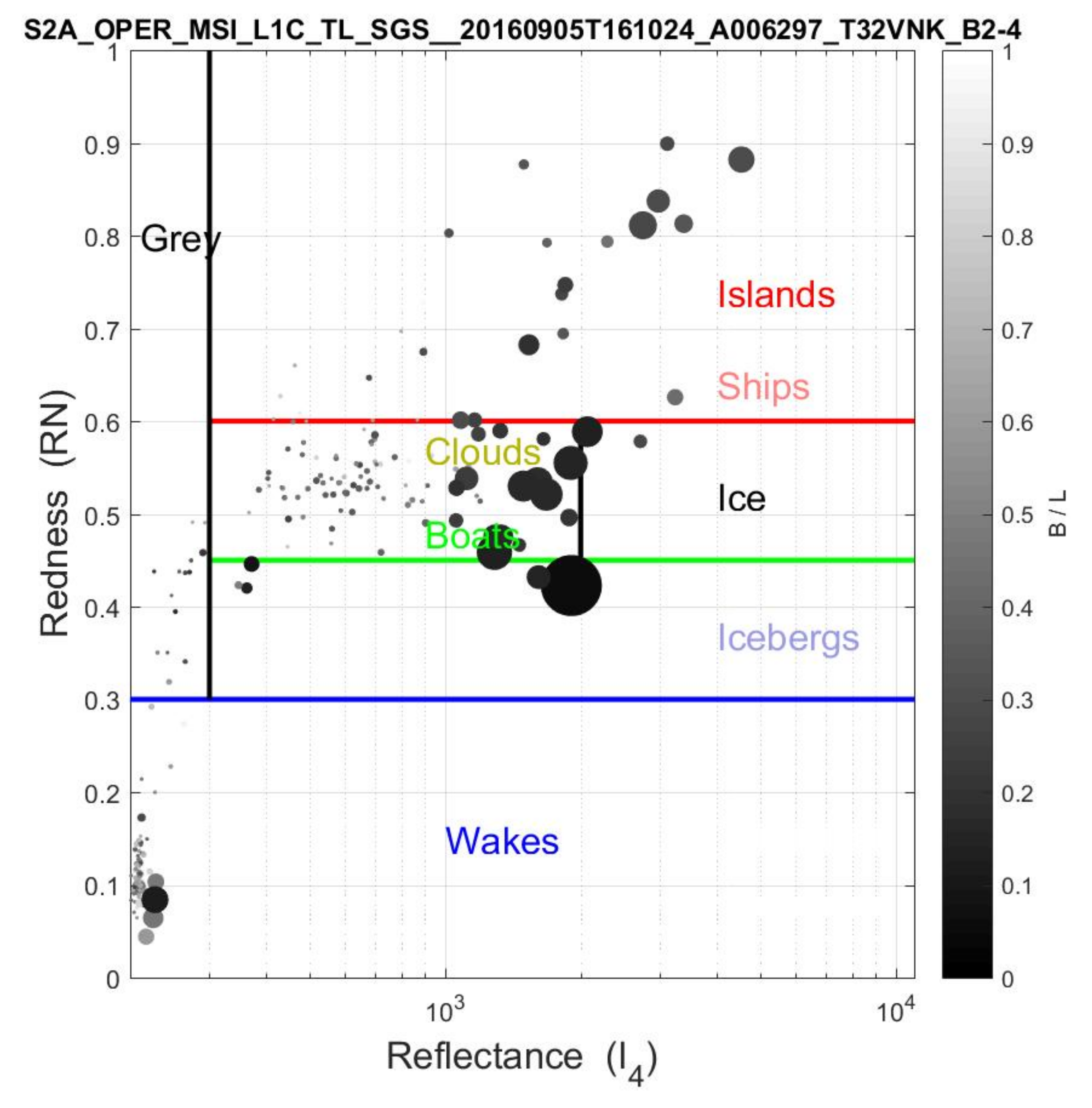
Another useful quantity is the “redness”, defined as the reflectance in the red and near-infrared with respect to the total reflectance

$$\mathrm{RN}\left(s\right) = {\frac{{\mathrm{I}}_{\mathrm{B}4}\left(s\right)+{\mathrm{I}}_{\mathrm{B}8}\left(s\right)}{{\mathrm{I}}_4\left(s\right)}}_{}$$

(6)

The multispectral imagery is mostly reflected sunlight. Cold objects tend to absorb more red and infrared light whereas warmer objects absorb some of the blue light, and reflect and emit more red and infrared light. For example, wakes and ice floes are cold with low redness whereas large ships, islands and land generally seem warmer with higher redness. The redness RN is therefore a good classifier, and we define the following four classes:

• Red: 0.6 < RN < 1
• Yellow: 0.45 < RN < 0.6
• Green: 0.3 < RN < 0.45
• Blue: 0 < RN < 0.3

These RN classification parameter values were determined by minimizing the number of false alarms, i.e., off diagonal elements in the confusion matrix as discussed in Section 4, and thereby optimizing the classification algorithm. This color classification follows the visual spectrum and is shown in the color bars of Figure 4 and Figure 9a, where the segments in the scatter plots are colored accordingly. The dashed lines next to the color bars show the class distinctions.

Total reflectance and redness are just two classifiers based on the 13 spectral reflectances of the object. In a more general 2DPCA, we find that the two principal spectral components are indeed the total reflectance and the redness. A ship may have various colors but generally, its higher redness discriminates it from wakes, icebergs and grey ice.

A similar result has been found to be very useful in the analyses of vegetation and forestation [21,22]. In that case, the crops and trees all have a reflection that varies more or less linearly with spectral band wavelength but with different slopes. The slope is the principal parameter that can discriminate between the different types of crops and trees. The redness parameter NR is in our analysis very similar to this slope parameter.

Other bands also provide additional spectral details. For example, snow and, in particular, clouds have higher reflectance in the infrared bands B11 and B12. Accordingly, we define the infrared classifier

$$\mathrm{IR}\left(s\right) = {\frac{{\mathrm{I}}_{\mathrm{B}11}\left(s\right)+{\mathrm{I}}_{\mathrm{B}12}\left(s\right)}{{\mathrm{I}}_4\left(s\right)}}_{}$$

(7)

Since the segments have pixel resolutions of 10 m, the infrared bands B11 and B12 with 20 m resolution are pansharpened by dividing each infrared pixel into four weighted by the reflectance I₄ in the corresponding four pixels. More elaborate pan-sharpening methods, such as in Ref. [25], may be investigated in the future.

The l = 60 m low-resolution bands B1, B9 and B10 are useful for detecting aerosol, water vapour and cirrus clouds respectively, but we do not use them is this analysis as we are primarily interested in classifying smaller objects such as ships and icebergs. For this reason we only find minor effects of our atmospheric correction using the sen2cor algorithm [24]. In addition, the background subtractions, threshold, and relative reflections and band ratios, and the spatial classification reduce the effect of atmospheric corrections at least in the images analyzed in this work.

3. Classification Results

In each image I₄(i,j) all connected segments s = 1, …, N_s are identified as described above. For all segments their position, length, width, area, convex area, circumference, spectral reflectances in the four high-resolution bands and the resulting total reflectance, redness and infrared classifiers are calculated and listed. This information provides the basis for classifying each segment as one of the following objects: sailing ship, a slow ship or boat, island, iceberg, grey ice, wake or cloud. Each segment is assigned a number referring to a list with detailed spatial and multispectral parameters. The number is plotted on top of segments in Figure 2, Figure 6, Figure 7 and Figure 8 and Figure 10, and the color and size of the number classifies the segment as a specific object (see Figure 2), as a ship + wake, ship, boat, island, wake, iceberg or grey ice.

3.1. Wakes

Wakes appear in two forms in the S2 imagery. Breaking waves are found all along the west coast of Skagen in Figure 1 and Figure 7b. These waves are generally small and very cold and are seen in the scatter plots of Figure 2 as numerous small blue circles and in the scatter plot of Figure 4 at very low redness. Another type of wakes are those made by fast ships. These wakes often connected to the ships and very elongated and are classified as ship + wakes as will be discussed below. However, in a number of cases, large ships and catamarans make very long and wide wakes (and Kelvin waves) that split up in separate wakes. These wakes are not quite as cold as breaking waves and may be misidentified as discussed below.

3.2. Sailing Ships

Ships sailing fast enough create a long wake trailing behind [13,16,17]. The ship and wake are seen as distinct elongated objects with very small width to length ratio, typically B/L < 0.25, as shown with purple line in Figure 2. We classify these as ship + wake based on B/L alone. Their area is usually medium to large. The classification is independent of spectral properties as they can have all colors as seen in Figure 2, and their total reflectance is usually medium to large.

We do, however, find erroneous classifications in Figure 8 from elongated drifting ice floes but, as will be discussed below, they often curve spatially and can be declassified for that reason.

In Figure 7b, a large ship is sailing fast and at the same time turning sharply around the Skagen reef whereby part of its wake is separated from the ship. Since the wake curves, it is not classified as a ship, although it is elongated and matches spectrally. Instead, it is classified as ice according to the criteria described above. However, as it spatially is a continuation of a ship + wake, we can identify it as a wake. This example shows in detail how the classification works and how additional spatial information can be exploited intelligently. Alternatively, one might a priori assume that there are no icebergs in south Denmark, however, then, the classification algorithm would not work in the Arctic with the same set of classification parameters.

The above examples show how the detailed physical understanding of the objects can be exploited to improve the classification.

3.3. Ships and Boats

Ships are elongated and we use the observed ratio B/L as a spatial classifier for ships. Spectrally, we find that the ships have medium to large redness, generally such that smaller boats are green with 0.45 < RN < 0.6, whereas larger ships are red with RN > 0.6. This subdivision is not important for ship classification but is practical since we anyway make this spectral subdivision for ice and islands for larger ratio B/L as discussed below.

We also find that grey ice has a lower reflectance than most boats whereas icebergs have a higher reflectance than boats. Therefore, the reflectance I₄ can be used to discriminate and classify these objects.

3.4. Islands

Islands come in all sizes and shapes but most have area larger than ships and shape less straight and elongated than ships and therefore larger B/L. In addition, their temperatures are often larger resulting in a redness above RN > 0.6, which is indicated by the red dashed line on the color bar of Figure 4.

In Figure 7b and Figure 10, a few large ships have fuel ship along side and therefore appear twice as wide. These are on the border of being identified as islands. The discrimination parameter r = B₀/L₀ for the ratio of the ship breadth and width must therefore be chosen carefully.

As seen in Figure 2 and Figure 8, several islands around Nuuk are correctly classified but a few are not detected. If the islands are too close to land, their segment may not be separated from the land due to ice floes clogging the narrow straight between them. In another case, two close-by islands cannot be separated and are mis-classified as a long ship. These and other false positives and negatives can be removed by adjusting the threshold for segment identification, however, at the cost of losing some low reflectance objects close to the threshold.

3.5. Icebergs

Icebergs also come in all shapes and sizes. Spectrally, they are distinguished by having high reflectance and being cold. On the redness scale, they are green 0.3 < RN < 0.45, as seen in Figure 9. A number of icebergs are found and correctly classified in Figure 2 and Figure 8.

3.6. Grey Ice

Ice comes in many forms, reflectivities and textures, and can be classified into subclasses such as new ice, slush ice (nilas), young ice, grey ice, grey-white ice, first year ice, first year thin ice, second year ice and multi-year ice. Eskimos have several dozens of different words for various types of ice with and without layers of snow. Ice appears in increasing area and number during winter in the Arctic particular in polar regions and in the ocean around Northeast Greenland, Jan Mayen and Svalbard. Reflection and form vary with the age of the ice and underlying ocean currents.

As we are mainly interested in ships and icebergs, we classify all the above types of ice in one class that simply will be referred to as “grey ice”. It appears as low intensity textures in the sea and near the coast in the S2 winter images of Nuuk. Grey ice is not as highly reflecting (white) as icebergs but can be as cold.

The grey ice may be thin and widespread and appear grey with low I₄ as in the case of Figure 8a,b. It is therefore advantageous in such cases to increase the threshold in order to reduce the amount of sea ice objects and area. Instead other objects as icebergs, islands and ships appear which otherwise would have been connected spatially with grey ice.

As mentioned above, we find that the convex area is a very useful spatial classifier for objects. We find that ships and round objects such as some islands and icebergs have convex area about same as the observed area, whereas ice floes and clouds often curve or have irregular surfaces. The resulting larger convex area successfully discriminates in particular ice floes from ships. Unfortunately, we also find exceptional cases where a fast and turning boat makes a curving wake that therefore is mistakenly identified as an ice flow but these can be spatially correlated with nearby ship + wakes.

3.7. Clouds

Clouds obscure the S2 imagery [13] depending on weather, geographical coordinates, time of year, etc. For example, clouds cover Greenland about half of the time all year. Dense cloud cover renders the imagery useless and even degrades S1 SAR imagery. Despite this, often the cloud cover is only partial and is then useful to classify clouds. They come in all shapes and are generally white with redness within 0.45 < NR < 0.6 and therefore difficult to discriminate from boats [10,11] and ice floes. The S2 image in Figure 10 was selected because it contains a large number of smaller clouds, which challenge the classification algorithm. By visual inspection, one can distinguish ships from clouds from more complex texture features. We have thus far only included the spectral and spatial classifiers as described above, but can foresee further improvements of our physical classification algorithm embodying a number of more complex object texture features as for example described in [10] or as widely employed in large area SAR imagery [2].

Another way to discriminate clouds is through their infrared signature IR, which we find is larger for clouds than surface objects such as boats and ice floes generally. We find that clouds generally have IR > 0.45 and therefore use this classifier to separate them from ice floes, boats and other objects that have IR < 0.45.

3.8. Algal and Sea Clutter

Some sea clutter, algal blooming and sea current sediments are seen near the coast in Figure 1, Figure 7 and Figure 10. They only exceed the background threshold in a few cases, which are classified as grey segments. For reasons of simplification, we ignore these few cases. In the future, we intend to extend the classifications to include algal, oil spill, pollution, windmills, oil rigs and other objects in the sea.

4. Confusion Matrices, Classification Accuracy, False Positives and Negatives

For each of the S2 images, the classification algorithm results in a number of segments in each class as described above. Each segment is subsequently identified as an object from a priori knowledge of the images. For example, we know where the islands are situated, and that breaking wakes are found along the coastline. Furthermore, we know that in the Skagen images the remaining objects are mainly ships or clouds since there are no icebergs or grey ice. On the other hand, in the Nuuk images, we can identify the few fishing boats as they all are sailing out of the harbor with long ship wakes trailing behind. The remaining objects are islands, icebergs or grey ice.

Although this object classification is different for the Skagen and Nuuk images, the classification algorithm is the same and with the same spectral and spatial classification parameters. The only difference is the threshold and greyness parameters, which are larger in the Nuuk images because the widespread ice floes have low reflectances.

In

Table 1. Confusion matrix for classifications from the Skagen area, Figure 1 and Figure 7a,b and Figure 10. First column lists the object classes and first row the segment classes (see text). Diagonal numbers are correct identifications and non-diagonal numbers are mis-identified (confused) as false positives or negatives.

Skagen Denmark	Ship + Wake	Ship	Boat	Island	Icebergs	Wake	Grey Ice	Cloud	Total	PA
Ship + Wake	25	0	0	0	0	0	0	0	25	1
Ships	0	18	0	0	1	0	0	0	19	0.93
Boats	0	0	61	5	0	0	16	8	90	0.68
Islands	0	0	0	2	0	0	0	0	2	1
Icebergs	0	0	0	0	0	0	0	0	0	-
Wakes	0	0	0	0	1	82	5	0	88	0.93
Grey ice	0	0	0	0	0	0	0	0	0	-
Clouds	0	0	0	2	0	6	0	173	181	0.96
Total	25	18	61	9	2	88	21	181	405
UA	1.0	1.0	1.0	0.22	0	0.93	0	0.96		0.89

, we show the confusion matrix for all segments and objects in S2 images (Figure 1, Figure 7a,b and Figure 10) of Skagen and in

Table 2. Confusion matrix as Table 1, but for the Nuuk area in Greenland, Figure 2 and Figure 8a,b.

Nuuk Greenland	Ship + Wake	Ship	Boat	Island	Iceberg	Wake	Grey Ice	Cloud	Total	PA
Ship + Wake	17	0	0	0	0	0	0	0	17	1.0
Ships	0	1	0	0	0	0	0	0	1	1.0
Boats	0	0	4	0	0	0	1	0	5	0.80
Islands	0	3	0	12	0	0	0	0	15	0.80
Icebergs	0	0	0	0	172	0	0	0	172	1.0
Wakes	0	0	0	0	1	0	0	0	1	0
Grey ice	0	0	21	0	0	3	20	3	47	0.43
Clouds	0	0	0	0	0	0	3	98	101	-
Total	17	4	25	12	173	3	24	101	359
UA	1.0	0.25	0.16	1	0.99	0	0.83	0.97		0.90

those from images (Figure 2 and Figure 8a,b) of Nuuk. The segment and object classification is described above. The classification parameters were chosen in order to maximize the number of correct identifications in the diagonal. Off diagonal numbers are mis-identifications or confused objects. False negatives lie above the diagonal and false positives (false alarms) below. Concerning ships and icebergs, one prefers false positives rather than false negatives in order not to miss any of these important objects.

In Figure 10, there are a great number of clouds present. Spectrally, they appear in the yellow class but most are not elongated spatially and can therefore be separated from boats. The infrared classifier IR of Equation (7) is particular useful for correct cloud classification as can be seen in Table 2. We validate the objects by visual inspection, since texture features distinguish the clouds from ships.

In Table 1, the last column lists the object detection probability also called producer accuracy (PA), i.e., the number of correct classification with respect to the total number detected of that object. Only in few cases is an object not detected and therefore the number of objects present is almost the same as the detection number. Last row lists the segment detection probability also called user accuracy (UA). For all three Skagen images the overall accuracy is OA = 89%. Ship + wakes, ships and boats are to a high degree classified correctly with PA = 100%, 93% and 68%, respectively, and UA 100%. Their performance factor F = 2 × PA × UA/(PA + UA) is F = 100%, 97% and 81% respectively.

We conclude that the classification algorithm is excellent for distinguishing ship + wakes, ships and wakes. About 32% of the smaller boats are confused with grey objects and clouds. This is because very small boats have low reflectance and may not be sufficiently elongated when they only extend over few pixels. If we had a priori excluded ice around Skagen, we would have identified them correctly as boats in these images.

In Table 2, we show the confusion matrix for Figure 2 and Figure 8a,b of the Nuuk area. Ship + wakes, ships, islands, icebergs and clouds are correctly classified to a high degree. In Figure 8b, grey ice appears in great numbers. Since the grey ice can appear in all forms and their number is large, a few also fall in green elongated class and are mis-identified as boats resulting in a low UA = 16%.

It is not always possible by visual inspection to distinguish icebergs and grey ice, and it is likely that some are confused. This is not cosnidered in Table 2. The confusion is not important as most ships stay away from both. If icebreaker ships need to distinguish, our algorithm must be extended. This would require ground truth information on positions of icebergs and sea ice in a given satellite image. Ship + wakes are classified well, PA = 100%, but some cold islands are confused with ships. The overall accuracy is OA = 90%

We learn from the supervised classification scheme applied to the Skagen and Nuuk images that small boats are difficult to separate spatially and spectrally from grey ice, especially because we have increased the grey ice parameter for the Nuuk images as compared to the Skagen images. The important lesson learned is that it will be extremely difficult to find small boats in grey ice if they lie still or are capsized. If they sail and create a wake, the boats and ships are easily detected and accurately classified in Sentinel-2 images.

5. Conclusions

Several sets of S2 MSI satellite images over Skagen, the northernmost tip of Denmark, and Nuuk, the capitol of Greenland, have been analyzed. Both contain a large number of ships and fishing boats as well as wakes, islands, icebergs, sea ice and clouds. The search and segmentation model finds all objects above a specified background. A supervised classification model was developed based on spatial and spectral classification parameters that have direct physical meaning. Detailed information on elongation, convex area, ship and wake correlations, allowed us to further improve and optimize the classification model which resulted in fewer confusions.

The most important parameters (principal components) are the area and elongation for the spatial part, and the total reflectivity, redness and infraredness for the spectral part. The first four parameters are implicitly represented in the scatter plots of Figure 4 and Figure 5 of all segments in Figure 1 from Skagen, Denmark, and likewise in Figure 9 from Nuuk, Greenland.

The optimal spectral and spatial classification parameters are the same for the satellite images analysed here. The only scene dependent parameter is the threshold which was increased in the complex Figure 8a,b to suppress the abundant sea-ice and cloud cover causing a number of false alarm. The scene dependent parameter is a weakness of the model, and should be upgraded by some automatic procedure.

Where large ships are very elongated, smaller boats fill fewer pixels and therefore generally less elongated. The total reflectance is larger for icebergs, islands, and larger ships and their wakes, whereas waves and small ships generally have smaller reflectance. Islands and large ships typically have high redness, whereas icebergs, wakes and especially waves appear rather blue. Smaller ships are more widely distributed between these limits and could be classified as boats if sufficiently elongated.

The classification model proved very useful for detection and classification of sailing ships, anchored ships, fishing boats, icebergs, grey ice, wakes, islands, and clouds. The resulting confusion matrices display between 93% and 100% correct classifications of ships and icebergs in the less complex S2 MSI satellite images without grey ice and clouds. However, the satellite images with abundant sea ice or clouds were very challenging as these objects can come in a wide variation of spatial and spectral forms, which led to a substantial increase in the number of false positives and negatives as described in confusion matrices.

The classification model was trained and optimized on most of the data including the complex images. Thus, validation on independent data was very limited. Consequently, the object classification may be overfitted and the diagonalization of the confusion matrices optimistic.

These results can be compared to recent S1 SAR images regarding the ship classification accuracy. A recent analysis of S1 Interferometric Wide Swath data [5] includes 27 SAR images containing 7986 ships in total. The resolution is 10 m × 10 m and thus comparable to the S2 MSI. Their optimal algorithm has a detection probability of 89% with 14% false detections, and a performance F = 0.87. Their images do not contain sea ice (or clouds) and should therefore be compared to the producer accuracy PA = 100% for ship + wakes and PA = 93% for ships in our multispectral S2 images. In this comparison, we note that most of the boats in the multispectral images are smaller compared to the 7986 ships analyzed in the SAR images. Furthermore, one should take into account that much of S1 SAR data over the Arctic is in the Ground Range Detected either Extended Wide swath mode with resolution 50 m × 50 m or Interferometric mode with resolution 20 m × 22 m, both considerably worse than in Ref. [5]. Other satellites can provide better resolutions SAR and optical images in narrower regions, but generally optical classification is considerably more accurate than SAR.

6. Outlook

An obvious extension of the object classification in marine and arctic environments from S2 MSI is to include all 13 multispectral bands and to use pan- or hyper-sharpening techniques [26] for the bands with lower resolution. Especially the infrared hyperspectral index IR was very useful for cloud discrimination.

Another extension is with regard to spatial and texture classification by exploiting further details of the spatial extent of the segments. For example, the curvature was useful for discriminating straight ship wakes from ice floes, and such shape and texture properties may be further exploited.

Additionally, a comparison to Sentinel-1 SAR imagery with two polarizations will provide complementary and weather-independent information although with substantial lower resolution (except in the rare and narrow swath SM GRD full resolution mode). The synergy of S1 and S2 imagery should be investigated for daily searching and tracking of ships, icebergs and ice floes.