Abstract
In this study, a new method is proposed for semi-automated surface water detection using synthetic aperture radar data via a combination of radiometric thresholding and image segmentation based on the simple linear iterative clustering superpixel algorithm. Consistent intensity thresholds are selected by assessing the statistical distribution of backscatter values applied to the mean of each superpixel. Higher-order texture measures, such as variance, are used to improve accuracy by removing false positives via an additional thresholding process used to identify the boundaries of water bodies. Results applied to quad-polarized RADARSAT-2 data show that the threshold value for the variance texture measure can be approximated using a constant value for different scenes, and thus it can be used in a fully automated cleanup procedure. Compared to similar approaches, errors of omission and commission are improved with the proposed method. For example, we observed that a threshold-only approach consistently tends to underestimate the extent of water bodies compared to combined thresholding and segmentation, mainly due to the poor performance of the former at the edges of water bodies. The proposed method can be used for monitoring changes in surface water extent within wetlands or other areas, and while presented for use with radar data, it can also be used to detect surface water in optical images.
Keywords:
water mapping; surface water; wetland; SAR; RADARSAT-2; histogram; threshold; segmentation; superpixel 1. Introduction
Wetlands provide a range of ecosystem services, including several that are vital to the health of the environment. Many species rely on wetlands, for example, to provide critical habitat used for procuring food and shelter. Wetlands also improve water quality by naturally filtering toxic substances and sediments. Unfortunately, these qualities were not well recognized in Canada until relatively recently, resulting in numerous wetlands in the south being filled or drained for other uses, including agricultural production [1]. Today, greater efforts are being made to protect these sensitive ecosystems. However, many are still threatened by the effects of anthropogenic disturbance [2], and of particular relevance to this study, climate change [3].
Increased variability and changes to ambient temperature, precipitation, and flow regimes are anticipated [3], and will likely adversely impact wetland ecosystems, which are especially sensitive to changes in the duration of flooding and depth of water [4,5]. Changes in the stability of flow regimes specifically may lead to the loss of suitable habitat for species that are adapted to certain levels of variation, and could lead to increased numbers of invasive and or generalist species [6]. In light of this, there is need for regional monitoring of changes in the extent of surface water within wetlands as this will help identify those areas that are changing. Not only would this inform management strategies, but it would also focus conservation efforts, which would be especially beneficial to those for which wetlands provide habitat and who are already at risk of extinction.
Surface water detection (SWD) using synthetic aperture radar (SAR) data has been the subject of study for many research groups [7,8,9,10]. SAR data is a reliable source of information for operational monitoring of water resources since, in contrast to optical data, images can be acquired regardless of cloud cover and haze. Further, due to predominant specular reflection, radar backscatter over non-disturbed water bodies is low relative to most surrounding land and other non-water features. This results in contrasting dark and bright pixels (between water and non-water features), a characteristic that can be used to discriminate both land cover types in SAR images.
Due to their simplicity, threshold-based procedures are widely used for operational SWD, particularly for large datasets [7,8]. Several techniques exist for finding an appropriate threshold value, the simplest of which includes scene-based visual investigation of histograms [11]. This approach is not practical for operational mapping however, as the threshold value differs under different incident angles, wind, and terrain conditions; thus, there is a need for human intervention on a scene-by-scene basis. Alternatively, Bolanos et al. [7] proposed using a normalized threshold value applied to energy texture images to extract surface water extents from RADARSAT-2 images (i.e., where is a non-dimensional threshold value standardized by the mean: , and standard deviation: , of the energy texture image, and is the threshold value before being normalized).
Statistical modeling of histograms has also been used in several cases to estimate a threshold value for automatic SWD. Matgen et al. [9] estimated the probability density function (PDF) of backscatter values for water using a gamma distribution and adapted an iterative procedure to define an optimal threshold value to separate water and non-water pixels while limiting over-estimation. Schumann et al. [12] computed threshold values for histograms using Otsu’s method [13] by applying a criterion to evaluate the between-class variance calculated from a normalized histogram. Notably, one of the limitations of Otsu’s method is that when the bimodality of histograms is unbalanced, the threshold value can over or underestimate the extent of water bodies as a result of the dominant mode having a greater effect on the between-class variance, thus resulting in the threshold being drawn closer to its mean [14,15].
To address this, Li and Wang [10] applied a modified version of Otsu’s thresholding algorithm to a subset of SAR-based texture (entropy) images. This modified version, called “valley emphasis”, attempts to select a threshold that is closer to the valley between the two modes. Li and Wang also subset images so that each contained between 10% and 90% water to ensure that the water and non-water modes of the histogram were more balanced. To do this, an initial water body mask is generated using K-means clustering applied to the SAR intensity image. Despite these advances however, the limitation of Otsu’s method remains, especially in cases where the population of water pixels is much lower than the population of non-water pixels.
It is notable that in the literature most SWD methods lack an ancillary process to reinforce the grouping of water pixels, especially along local boundaries between water and non-water features. Attempts to address this common deficiency have focused primarily on making slight adjustments to the threshold value in order to compensate for over or underestimation [9]. As an alternative, we propose the use of image segmentation via the simple linear iterative clustering (SLIC) superpixel method for improved SWD.
Image segmentation has increasingly become a key preprocessing step for computer vision applications such as object class recognition and image segmentation [16,17]. In general, existing algorithms are broadly categorized as graph- or gradient ascent-based approaches [18]. The former are useful for capturing image boundaries, while the latter are beneficial when a regular lattice is required. Achanta et al. [19] suggested three important properties for a desirable segmentation algorithm, including the fact that they are fast and easy to use while maintaining the quality of the results, and also that they adhere to image boundaries. The authors compared five types of superpixel algorithms (two graph-based and three gradient-ascent-based), including their newly developed SLIC superpixel algorithm. Their in-depth comparison showed that their proposed method, which is a gradient-ascent approach based on k-means clustering, outperformed other algorithms on all three aspects (i.e., speed, ease of use, and boundary adherence).
In light of these developments, we have developed a new method for SWD with SAR data that uses both thresholding and image segmentation based on the SLIC superpixel method. In this paper, the method is described in detail and results are demonstrated for multiple RADARSAT-2 images acquired over two study areas. The new thresholding method is based on the statistical characteristics of image histograms (or probability density functions), and select thresholds are applied to image objects. In contrast to previous SWD methods in which the cleanup procedure was implemented implicitly, we also describe a separate and fully-automated cleanup procedure and evaluate its impact on the accuracy of the algorithm.
This paper begins with this introduction followed by the a description of the study area and the methodology. The results are then presented and discussed followed by the conclusion.
2. Study Areas and Data Acquisition
Two study areas with temporally and spatially variable open water bodies are considered in this research (Figure 1). The first site (Figure 1b; referred to hereafter as the Prairie Pothole Region) was also evaluated by Bolanos et al. [7], and thus our newly proposed method was compared to their SWD method. For this site, a Radasat-2 Fine Quad Pol (FQ19) mode image with a nominal ground range resolution of 8.4 m (near-range) covering approximately 25 × 25 km was acquired on 8 September 2012. A same-day, cloud-free RapidEye image (5-m resolution) over Elk Island National Park, Alberta, was used to extract water polygons for comparison purposes using both methods (Figure 1a). Readers are referred to Bolanos et al. [7] for additional information on this site and dataset, which has not been repeated here for brevity.
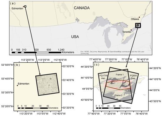
Figure 1.
(a) Study areas located in Canada, including (b) the Prairie Potholes Region in Alberta, and (c) the Bay of Quinte in Ontario. Both study areas are covered by concurrent RADARSAT-2 images and high-resolution optical images. The red polygon represents the overlap for two image frames available over the Bay of Quinte site. For the Alberta site only one RADARSAT-2 image was available.
The second study area covers the entirety of Prince Edward County and the Bay of Quinte, Ontario (Figure 1c; referred to hereafter as the Bay of Quinte site). This region is located on the Canadian side of Lake Ontario, falling completely within the Mixedwood Plains Ecozone [20]. Here, rainfall generally peaks in September around 90 mm, and temperatures peak in July at around 21 C (1981 to 2010 Canadian Climate Normals [21]).
With an abundance of fertile soils, the majority of land is used for agricultural production. Wetlands (marsh and swamp) are numerous, and the extent of water bodies varies extensively on an inter and intra-annual basis, both as a result of water level changes, and the emergence of vegetation from the water surface as the growing season progresses. For this site, 11 sets of images of RADARSAT-2 Wide Fine Quad Pol (FQ5W and FQ17W) were acquired between 7 April and 22 September 2016. Each scene covers approximately 50 × 50 km, with a nominal ground range resolution of about 14 (FQ5) and 9 (FQ17) m (Table 1). For accuracy assessment of this site, concurrent and cloud-free WorldView-2 (WVII) images are analyzed. Note that for a meaningful comparison between the results from the two data frames and all dates, we have only focused on analyzing the area covered by all image acquisitions for the Bay of Quinte (see Figure 1c).

Table 1.
RADARSAT-2 images acquired over the Bay of Quinte.
3. Methodology
3.1. Image Processing
Figure 2 summarizes the processing steps applied to available RADARSAT-2 imagery. Image calibration was performed via the extraction of Sigma Nought () values using the Constant-Beta look-up tables provided with each scene. A polarimetric Lee filter was then applied to compensate for the effects of speckle. Bolanos et al. [7] discuss the advantages of this filter over others due to its ability to adapt to homogeneous and heterogeneous areas, and its ability to preserve edges. This, in addition to the fact that we wanted to make direct comparison between our method and the method proposed by Bolanos et al., is why we also used the Lee filter in this study. All RADARSAT-2 images were then orthorectified using the rational polynomial coefficients provided with the images and a Shuttle RADAR Topography Mission (SRTM) digital elevation model (DEM). Afterward, all orthorectified images were co-registered using a fast Fourier transform phase matching algorithm with a minimum match score of 0.9 set for automatically selected ground control points (GCPs). These image processing steps were implemented using PCI Geomatics software. After orthorectification, the calibrated intensity values were then converted to decibels to pronounce the tails of each image’s histogram.
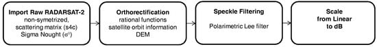
Figure 2.
The proposed workflow for preparation of RADARSAT-2 imagery. Note that the method could also be adapted to different processing methodologies, SAR data types, and optical imagery. SAR: synthetic aperture radar; DEM: digital elevation model; dB: Decibel.
3.2. Threshold Selection
With the proposed method, two sets of thresholds are extracted from the SAR images for two different purposes: (a) surface water detection; and (b) water boundary detection. For the former, histograms of either HH (Horizontal transmit and Horizontal receive) or HV (Horizontal transmit and Vertical receive) polarizations are used to select a statistically consistent threshold, while for the latter, higher-order texture images, such as variance, are used to select a threshold to detect the boundaries of water bodies. This latter step provides products for an additional cleanup process for the removal of false positives, or areas identified as water bodies, but which are not in fact water bodies. Each threshold type is described in detail in the subsequent section.
3.2.1. Surface Water Detection
Previous studies such as those of Brisco el al. [8] and Manjusree et al. [22] discuss the advantages of using the HH polarization for mapping flooded vegetation due to better canopy penetration, resulting in better contrast between flooded and non-flooded forests (e.g., compared to HV). Over non-disturbed water bodies, co-polarized channels are also used for discriminating land and water, though it is notable that at steep angles backscatter in the HH polarization can be equivalent to the values observed for land, and increased surface roughness (e.g., waves) reduces the separability between water and land [23]. Alternatively, several studies have shown that backscatter values of the cross-polarized channels HV and VH (Vertical transmit and Horizontal receive), are less affected by wind than the co-polarized channels [24,25]. In this study, we are interested in detecting water regardless of the roughness conditions; thus, have chosen to use the HV polarization. Note that this method could be adapted to use any polarization, as it relies solely on the fact that the distribution of values is bimodal (referring to the fact that image histograms show separate modes: one representing water, and one or more others representing non-water pixels).
Bimodality of image pixel values is typically achieved with a sufficient number of water bodies, with low backscatter values, relative to all non-water pixel values. Note that preliminary testing has demonstrated that bimodality can be achieved with as few as 2% of the total pixel population representing water. To define the threshold values, the values are first represented in decibel format (Figure 3a) as this representation is commonly used, and thus users can associate a given value with typically observed responses. This format also reduces noise and improves contrast [7]. In order to better visualize the low probability mode in the histogram, log scaling is applied to the vertical axis (Figure 3b). Then, a high-order polynomial is fitted to the dataset (Figure 3b), and the threshold is found at the local minimum, or valley, between the two modes (i.e., between the first mode, representing lower backscatter values, which typically represent water, and the second mode(s), representing higher backscatter values, which typically represent non-water pixels).
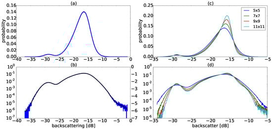
Figure 3.
Image histograms generated from the HV intensity values for a Wide Fine Quad Pol image acquired over the Prairie Pothole Region, including (a) histogram of backscattering intensity values in dB; (b) the same histogram as (a) with logarithmic scaling applied to the vertical axis (solid black line represents a 55-order fitted polynomial with its corresponding vertical axis in an arbitrary unit); (c) histograms that resulted from applying different window sizes of the polarimetric Lee filter; and (d) the same histogram as (c) with the vertical axis in logarithmic scale (histograms are plotted using 1000 bins).
Figure 3c,d show the effect of applying speckle filtering with different window sizes on the shape of the image distribution. Speckle filtering consists of reducing the variance of a speckled image to improve the estimation of its mean [26]. In particular, the Lee filter requires the calculation of an adaptive filtering coefficient based on the local statistics defined by a sliding window of N × N pixels, in which homogeneous areas are low-pass filtered but heterogeneous areas that include texture information, such as sharp edges and isolated point targets, are preserved [27]. Table A1 shows threshold values identified via the approach described previously for the image in Figure 4a after having been filtered using various window sizes. Note that the threshold value increases as the window size increases (Table A1). This is mainly due to the average (low-pass) filter that causes an increase in the population of pixels identified as non-water while sliding over regions that are close to water edges. Thus, the thresholds calculated from images filtered with a larger window size can potentially lead to underestimation of the extent of water bodies as a result of increased mixing of land and water pixels. This is also reflected in the number of pixels selected as water, which are listed in Table A1. As such, for all images the polarimetric Lee filter with a 5 × 5 window size is used in this study.
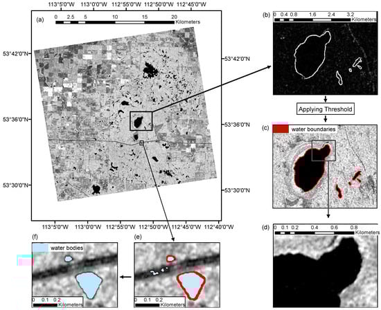
Figure 4.
(a) HV polarization image from the Fine Quad Pol mode 19 (FQ19) scene acquired over the Prairie Pothole Region; (b) variance texture image; (c) extracted water boundaries by applying a pixel-based threshold (1.1) on the variance image; (d) segmented image generated using the simple linear iterative clustering (SLIC) superpixel algorithm; (e) water bodies generated using thresholding and superpixel segmentation; and (f) final water bodies after topological intersection of detected water bodies and water boundaries.
3.2.2. Surface Water Boundary
Smooth features such as roads, as well as areas that are affected by shadow, tend to exhibit low backscattering returns, and thus are potentially falsely identified as water via simple thresholding processes. Therefore, we apply a cleanup procedure following the detection of surface water. To do this, we use the boundaries of water bodies that are detected via high-order texture images, specifically the variance of the HV intensity image. Variance is used in this case because backscatter values observed for smooth water bodies are relatively low, and show high homogeneity, whereas backscatter values for land are generally higher. Thus, high variance values are expected when the sliding window within which they are calculated includes both values for water and non-water features (i.e., at the boundary of water bodies).
Variance images were therefore generated from the same cross-polarized channel (i.e., HV) and were similarly log-transformed to pronounce the rare events at the high tail (Figure 5a–c). Given that the histogram of variance image values similarly exhibited a bimodal distribution (Figure 5d) we use the same procedure as described in Section 3.2.1 to define the threshold value (i.e., 1.1) at the local minimum between the two modes. Note that in this case, the mean and standard deviation of the total pixel population are and , respectively, and thus the threshold value () is approximately three standard deviations from the mean, i.e., (or ). Given the availability of a temporal stack of SAR images over the same area acquired at the same incident angle, the variance values of water pixels (and therefore all non-water pixels as well) are expected to be within the same range. Thus, we theorized that a constant value could be used for thresholding variance images at different times, and in cases where histograms of variance image values exhibit weak bimodality (i.e., we theorized that not all variance images need to exhibit strong bimodality to be used in this automated cleanup procedure). We investigated this hypothesis further in the results and discussion section.
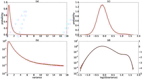
Figure 5.
(a) Histogram of the variance texture image from the Prairie pothole site, calculated using the HV polarization image from the Wide Fine Quad 19 scene; (b) the same histogram with the vertical axis in logarithmic scale; (c) log-transformed histogram of the variance image and (d) the same histogram as (c) with the vertical axis in logarithmic scale (histograms are plotted using 1000 bins, and colors as in Figure 3).
3.3. Superpixel Segmentation
The SLIC superpixel algorithm was used to group adjacent pixels with similar characteristics. Via trial and error, it was found that splitting the image into 1000 × 1000 pixels blocks with 3600 superpixels in each block worked best for identifying potential water bodies, regardless of their size. In this study, the SLIC superpixel algorithm is implemented using the open-source “skimage” Python package applied to the HV intensity image. The “compactness” and “sigma” parameters in all cases were set to 1, since this tended to produce the best results, and permitted detection of water bodies as small as 25 m. The former parameter balances the color and space proximity, with high values giving more weight to the former, resulting in superpixels that are more square. The latter parameter, sigma, is the width of Gaussian smoothing kernel, where a value of zero does not apply any smoothing and higher values apply more smoothing.
3.4. Surface Water Extraction
To generate final surface water products, first, the intensity image is segmented and pixel values are averaged over each superpixel. Then, the mean value is compared with the threshold value defined previously in Section 3.2.1 (to identify surface water). Superpixels with mean values lower than the threshold are selected as water. At this stage, the selection of water pixels is reinforced through two mechanisms: (a) by grouping pixels through the SLIC algorithm to ensure adherence to local boundaries; and (b) by applying the threshold on the average of grouped pixels (i.e., superpixels).
Subsequently, to improve accuracy, water boundaries extracted from thresholding of the variance image are intersected with features identified as water bodies (Figure 4e), and only those that are adjacent to boundaries are included in the final surface water product. In this research, this step is referred to as the cleanup procedure. Figure 4e,f exemplify this process, showing where some of the polygons incorrectly identified as water over a road are excluded from the final surface water product. Figure 6 summarizes the processing steps of the entire SWD workflow. It consists of two separate sub-workflows: the first one (the top line in Figure 6) is the thresholding and segmentation process which results in the generation of water objects; the second one is a boundary detection process (the bottom line in Figure 6) which results in the generation of water boundary objects. The cleanup process is the last step in which a topological intersection between the water objects and boundary objects is performed to remove false positives. In the rest of this paper, the cleanup process is referred to as the process of generating boundary objects and the topological intersection between boundaries and water objects. It is notable that the energy texture image [7] can also be used instead of HH or HV images as an input to the algorithm. Note that that there is no user intervention required in the workflow in Figure 6 since the all workflow can be automated, including the threshold selection process for both surface water and boundary objects. The only user intervention required in the present method is the separation between the single mode and bimodal (or multi-modal) histograms which has to be done after preparation of SAR imagery (i.e., after the process outlined in Figure 2 and before the workflow in Figure 6). As mentioned in Section 3.2.1, a biomodal distribution can be achieved with as few as 2% water pixels in the SAR imagery.
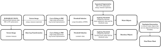
Figure 6.
The proposed workflow for surface water detection using RADARSAT-2 imagery. PDF: probability density function.
To assess the accuracy of the proposed method, water bodies were manually digitized from a WVII image collected on the same date as one of the RADARSAT-2 scenes (i.e., 27 April 2016). We believe these results to be the most accurate estimate of the true areal extent of surface water and thus results from the proposed method were compared to those values.
4. Results and Discussion
4.1. Bay of Quinte
As described previously, the proposed SWD method is a two-step process. First, thresholds for each frame are determined, and second, thresholds are applied to segmented images. The results of the first step, including the normalized threshold values (), are shown in Table 2 and Figure 7 for each frame for the Bay of Quinte. It is notable that in Table 3 the threshold values are quite different from one frame to another, demonstrating that a constant (normalized) threshold value is perhaps less suitable for analysis of temporal data. It is also interesting to note that in Figure 7, the histograms in May and June have an extra mode between water and the dominant non-water mode. This extra mode peaks at approximately at −20 dB, and represents emerging vegetation. Note that this observation was validated via available WorldView data collected throughout the 2016 growing season.
Table 2.
Threshold values for RADARSAT-2 HV polarization images at different dates and the area of detected surface water extents in the overlap area shown in Figure 1 over the Bay of Quinte (acquisitions in 2016). Digitized water extent in the overlap area is 81.091961 km; all areas are in km.
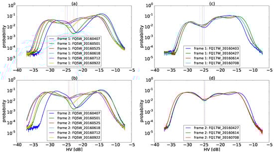
Figure 7.
The distribution in log scale of HV backscatter values over the Bay of Quinte on different dates and for each frame for the FQ5 (a,b) and FQ17 (c,d) modes. Dotted lines represent the local minimum value of the polynomial curve, representing individual threshold values. The threshold values are also listed in Table 2.
Table 3.
Difference in the areal extent of water bodies, in percent, after applying the cleanup procedure and using different variance threshold values. is the area of water extracted following a manual cleanup of results for each date.
The histograms of the variance texture measure of all frames are plotted in Figure 8. Note that there are many cases in which the distribution of the variance image is not bimodal due to a low population of boundary pixels. Based on these results we investigated whether a constant threshold value could be used for all variance images, given the homogeneity of water bodies and their low backscatter values, relative to the high backscatter from non-water features around water bodies. Four different threshold values were applied on the variance images. Based on the results of the Section 3.2.2 (in which was found 1.1) and the visual investigation of the plots in Figure 8, threshold values of , and 1.3 were evaluated.
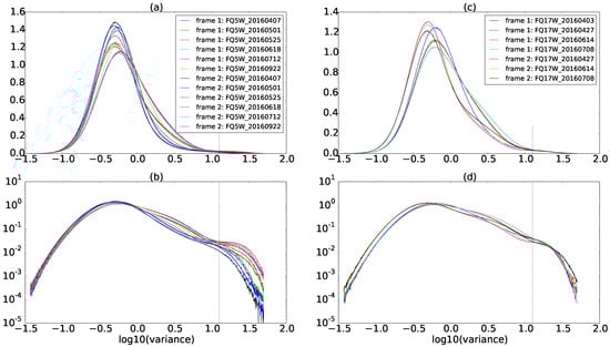
Figure 8.
The distribution of variance texture images over the Bay of Quinte at different dates at two different incident angles. (a) Wide Fine Quad mode 5; (b) the same histogram as (a) in log scale; (c) Wide Fine Quad mode 17; and (d) the same histogram as (c) in log scale (dotted lines represent the place of threshold for variance texture images, ).
Table 2 shows the areal extent of water calculated before and after applying the cleanup procedure. Note that before applying the cleanup procedure, the areal extent of water calculated for each image does not show a trend that is consistent with water level gauge information collected at several sites throughout the study area. Water heights increased throughout April, then mostly decreased until reaching September climate normals (ECCC, 2017). This discrepancy is a result of the true extent of surface water being masked by false positives. After applying the cleanup procedure however, accuracy is improved as demonstrated by the fact that the extent of surface water is closer to the values from the manually digitized surface water product, which we believe to be the most accurate estimate of the true areal extent of water. The results of the cleanup procedure are discussed later in this section.
Table 3 shows the percentage of falsely detected water bodies relative to the areal extent of water calculated via manually cleaned up products. For comparison, we use the non-dimensionalized variable , where A is area in km and is the best approximation of the true areal extent of water based on thresholding/segmentation, as well as manual cleanup procedures based on visual comparison to the WorldView image acquired on the same day (see Table 2 for values). These false positives are usually generated because of the presence of permanent or non-permanent smooth features (such as roads, airports, agricultural lands, etc.). The results in Table 3 show that by increasing the value of the threshold, the total area of detected water bodies after the automated cleanup procedure is closest to the . However, this improvement comes at the expense of losing some water bodies that were correctly identified. In other words, as we decrease the variance threshold, false positives increase, but if the boundary conditions are too relaxed (i.e., as we increase the variance threshold value) water bodies that do not have very distinct boundaries are also not detected.
To determine the appropriate threshold value, we calculated the percent of water losses using a variable , where represents our most accurate estimate of the areal extent of water based on the automated cleanup at , plus a manual cleanup procedure based on visual comparison of the WorldView image acquired on the same day. The difference between the two variables and represents the area of real water polygons lost due to the cleanup procedure. These results show that the real water extent losses due to an increase in value, for example at = 1.3, are as low as 0.03% (Table 4). For a better comparison, the percentage of false positives and the percentage of real water losses are plotted vs. the different variance threshold values in Figure 9. The plot suggests that the slight variation of the threshold value has only a minor effect on removing correctly detected water extents. On the other hand, it illustrates that a slight increase in the value of variance threshold value (as small as 0.1) removes additional false positives at a much greater rate. Thus, this demonstrates that using a constant threshold value for image variance is justifiable for SWD using SAR data, as the increase in the value of the variance threshold removes more false positives, but relatively few correctly-identified water bodies. More details on the accuracy of these results are discussed in the next subsection.
Table 4.
The variation of the detected area, in percent, after cleanup procedure using different thresholds.
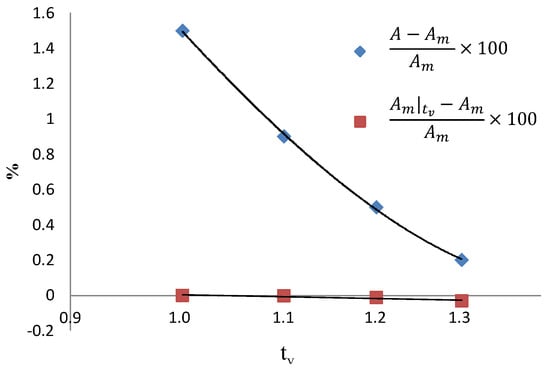
Figure 9.
The percentage of false positives (blue diamonds) that were removed and the percentage of true water polygons (red rectangles) that were removed for different variance threshold values. Solid lines represent fitted curves to the data.
Finally, it is notable that the areal extent of water extracted after the manual cleanup from the two frames shows a less than 0.4% difference for the two different incident angles at different dates (Table 2). This is a satisfactory result that suggests the SWD method proposed in this study can produce accurate and reliable results for images acquired at different incidence angles.
It is worth mentioning that after visually inspecting WVII images acquired in April, May, June and July, it was observed that floating and/or emerging vegetation was present at several sites beginning in May, but was not detected until June. This is because these features were much smaller in size than the incident microwaves and did not affect backscatter intensity. On 27 April specifically, these features were not visible, and thus did not affect the accuracy assessment completed in this study. Further discussion on floating and or emerging vegetation and its effects on SWD in the context of this study are presented in Section 4.3.
The accuracy of water bodies extracted after the thresholding/segmentation step is affected by two types of errors: false positives and overestimation (or underestimation). The suggested cleanup process was used to improve accuracy by removing false positives. The overall effects of different (variance) thresholds on the removal of false positives have been evaluated and quantified in terms of the percentage of false positives that were detected versus losses of correctly-identified water bodies (see Table 3 and Table 4 and Figure 9). To further investigate the details of such losses during the cleanup process, we have listed the number of true water bodies and the area of the largest one lost among those in Table 5. The number of lost polygons consistently increases as the variance threshold increases, but all of the lost polygons are very small water bodies. In many cases, these small water bodies did not exhibit distinct land/water contrast (for SAR data, speckle filtering can reduce the contrast between bright and dark features, especially if they are relatively small in size) and as a result their boundaries were not detected by the variance image. Given the accuracies of water products presented in Table 3 and Table 4 and Figure 9, we conclude that a threshold value between 1.1 and 1.2 offers a reasonable balance between the removal of false positives and the loss of real water polygons. However, this can be adjusted for specific applications by users; for example, those that are interested in minimizing the loss of small water bodies can use a lower variance threshold value around 1.0 (though this would be at the expense of more false positives). It is notable that the removal of the false positives, in general, is an easier task to deal with as other ancillary data can be used to mask permanent features (e.g., roads).
Table 5.
Overestimated and underestimated water extents over Fish Lake. All area estimates are in given in square meters.
Table 4 provides the number of water bodies that were detected after the manual cleanup of the water product generated for the scene acquired on 27 April. Interestingly, the number of detected polygons using thresholding is lower than those detected using thresholding/segmentation (72 and 81, respectively). This is an important observation, as it shows that the thresholding of segmented SAR images improved the number of correctly detected water bodies. Another observation is that the total area of detected water bodies using only thresholding is lower than that detected using thresholding/segmentation. This is in addition to the fact that the largest polygon lost in thresholding had a relatively small area (1288 m) and the percentage of difference (i.e., ) between the area of the manually cleaned up products from thresholding and thresholding/segmentation approaches is the highest percentage (−0.7) in Table 4.
This clearly suggests that the accuracy of water products generated using thresholding (but not segmentation) is further affected by underestimation of water extents compared to the products generated from thresholding/segmentation. As an example, we have calculated over and underestimated water extents on Fish Lake in the Bay of Quinte (see Figure 10, right). The areal extent of water found using the two approaches are listed in Table 5. The results show that the total area estimated from either approach is less than the true water extent, and that the detected water extent by thresholding is less than that of the thresholding/segmentation approach. We consistently observed this improved performance of the thresholding/segmentation approach compared to the thresholding only approach. The main reason for this improvement is the segmentation process, which is better able to detect the edges of water extents, and which rarely misclassifies the center of water bodies or the edges of scenes which may be noisy or represent slightly higher intensities from waves.
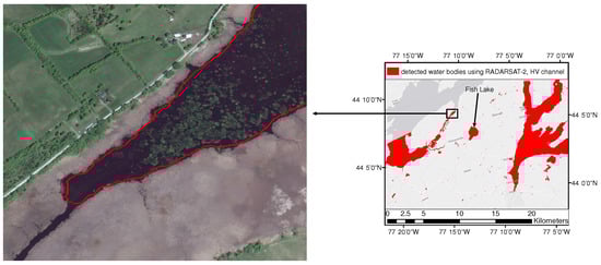
Figure 10.
An example of floating and or emerging vegetation from the WorldView-2 (WVII) image acquired on 22 May 2016; the red line represents surface water extent detected using the RADARSAT-2 image acquired on 14 June 2016.
We have also plotted the distribution of the areas of detected water bodies in Figure 11 for the three cases listed in Table 5. These histograms show that both thresholding and thresholding/segmentation approaches are less accurate in detecting water bodies with areal extents between 100 and 1000 m, but perform well in detecting water bodies larger than 10,000 m. Given the resolution of these data, and the requirement for speckle filtering, this observation is sensible. Specifically, it is reasonable that smaller water bodies cannot be detected as often the filtering processes result in the mixing of adjacent land and water pixels, thus reducing the difference between values, and subsequently the ability to differentiate them.
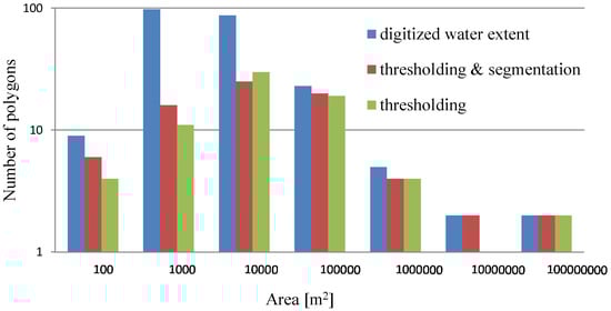
Figure 11.
Area distribution of water bodies within the overlap area for the Bay of Quinte site. The total number of polygons for the digitized water extent (blue) is 225, for thresholding and segmentation (red) it is 75, and for threshold only (green) it is 72.
4.2. Prairie Pothole Region
Table 6 and Figure 12 summarize results for the Prairie Pothole Region. Similar to what was observed for the Bay of Quinte, the results in Table 6 suggest that the extent of water detected using only thresholding is an underestimation (by about ) compared to the products extracted from thresholding and segmentation. As an example, the areas of open water calculated over Astotin lake using thresholding and thresholding/segmentation methods are 3.70 and 3.76 km, respectively. This 1.6% underestimation with thresholding only is again due to the poorer performance along the edges of water bodies, and the misclassification of pixels within the center of water bodies (Figure 13).
Table 6.
The number of polygons and detected surface water area over the the Prairie Pothole Region using the HV channel.
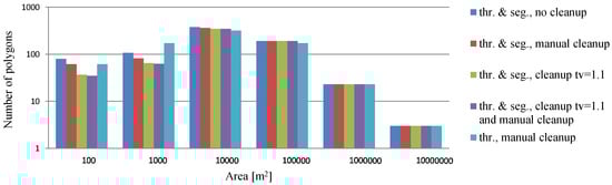
Figure 12.
Area distribution of the detected water extents over the Prairie Pothole Region.
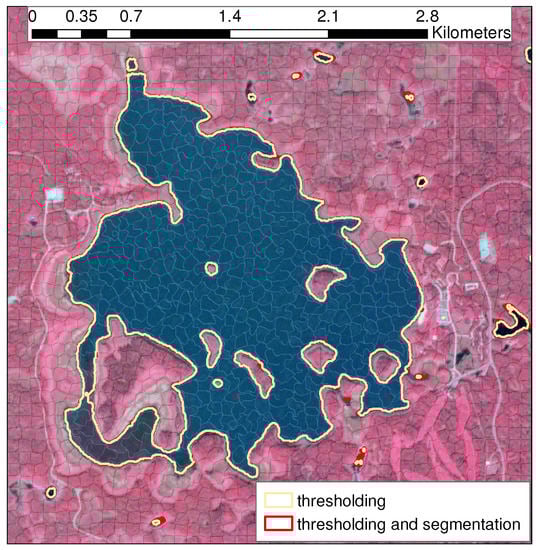
Figure 13.
Water extents from the RapidEye image; colored lines represent water extents generated using thresholding and thresholding/segmentation over Astotin lake.
In this case, the automated cleanup procedure improved the removal of false positives with the loss of very few true water polygons (29), which were all less than 1000 m; making up less than 0.15% of the areal extent of all water bodies. The numbers and sizes of water polygons found using the proposed method are provided in Table 6 and plotted in Figure 12. Two points can be highlighted regarding the histograms in Figure 12. First, the difference between the number of detected water polygons after applying the automated cleanup and automated/manual cleanup is very small, demonstrating that after the automated cleanup most false positives are removed. Second, the thresholding method in this scene shows a slightly better performance for water bodies in the range between 100 and 1000 m compared to thresholding/segmentation method. As mentioned previously, it is also possible to improve the accuracy for these small water bodies by decreasing the variance threshold, though at the cost of an increased number of false positives.
It is notable that the total surface water extent extracted by Bolonos et al. [7] is greater than the one calculated here (≃23 km). This difference is a result of Bolanos et al. [7] using a threshold value that is lower (note that the pixel values are all positive in energy texture image; a lower threshold in the energy image is the equivalent of stating a higher threshold in HV channel) than the value at the valley between the two modes of the energy image histogram. Further, the threshold values in their study were normalized values (i.e., subtracted from the mean and divided by standard deviation of the total pixel population), thus a small variation in the normalized threshold value () is translated to a greater change in non-normalized values ().
4.3. Limitations and Future Work
The SWD method proposed in this study can be used to generate seasonal, annual, or long-term permanent and non-permanent water masks using SAR data. However, one notable limitation is the inability to detect vegetation in standing water that is much shorter and thinner than the wavelength of incident microwaves. For the Bay of Quinte site specifically, it was observed that when floating and/or emergent vegetation first appears at the beginning of the growing season, it was sometimes still detected as water with the proposed method (Figure 10); however, as both the density and height of features increased through time, they were eventually classified as non-water pixels. Characterization of this type of temporal inaccuracy is complicated using SAR data as the roughness, height, and volume of this floating and/or emerging vegetation vary spatially, especially among different species. We propose that further improvements to this method can be achieved by incorporating information from high-resolution optical images. However, collecting coincident cloud-free imagery may not be possible in all cases.
5. Conclusions
In this study, a new method for semi-automated SWD using SAR data has been described and evaluated. The approach focuses on automatically defining threshold values, identifying water bodies and edge features on a per-object basis, and implementing an automated cleanup procedure which has been demonstrated to improve accuracy compared to thresholding only. This approach is adaptive to images acquired at different incidence angles and dates, removing the need for human intervention on a scene-by-scene basis. Additionally, an independent cleanup procedure is proposed to remove features falsely identified as water. The cleanup procedure is based on the detection of water boundaries extracted by thresholding images generated from high-order texture measures such as variance. The results showed that a constant threshold value can be used for extracting boundaries, thus it can be used in a fully automated cleanup procedure. This method, despite its current and relatively minor limitations, remains an attractive option in cases where there is need for surface water information for a specific time period (e.g., to determine available waterfowl habitat in spring), and for mapping large geographical areas, because results can be generated automatically, and SAR data can be acquired regardless of cloud cover and haze. Environment and Climate Change Canada expects to implement this approach operationally for spatial and temporal detection and monitoring of surface water within wetlands.
Acknowledgments
The authors would like to thank Bhavana Chaudhary for digitizing WVII images to extract water extents over the Bay of Quinte. We would also like to thank Patrick Kirby for his assistance with interface development and Python scripting. The authors would like to thank the Canadian Space Agency for funding in support of the Data Utilization and Applications Plan project (DUAP).
Author Contributions
The initial idea of this method was suggested/developed by White and Behnamian. Banks and Behnamian performed the all analysis, interpreted the results and wrote the first draft of the manuscript. Chen suggested the implementation of the SLIC superpixel algorithm for segmenting SAR images and contributed in developing the segmentation part of the Python script. Banks, White, Pasher, Millard and Behnamian suggested/developed/implemented the validation procedure. Behnamian wrote the Python scripts. All authors advised on the contents and helped edit the original and subsequent versions of the manuscript.
Conflicts of Interest
The authors declare no conflict of interest. The founding sponsors had no role in the design of the study; in the collection, analyses, or interpretation of data; in the writing of the manuscript, and in the decision to publish the results.
Abbreviations
The following abbreviations are used in this manuscript:
| DEM | Digital Elevation Model |
| ECCC | Environment and Climate Change Canada |
| GCP | Ground Control Point |
| Probability Density Function | |
| RGB | Red, Green, Blue |
| SAR | Synthetic Aperture Radar |
| SLIC | Simple Linear Iterative Clustering |
| SRTM | Shuttle RADAR Topography Mission |
| SWD | Surface Water Detection |
| WVII | WorldView-2 |
Appendix A. Lee Filter and Window Size Effects on Threshold Values
Table A1.
Threshold values in dB for the HV polarization of the RADARSAT-2 image acquired over the Prairie Pothole Region filtered using a polarimetric Lee filter with different window sizes.
Table A1.
Threshold values in dB for the HV polarization of the RADARSAT-2 image acquired over the Prairie Pothole Region filtered using a polarimetric Lee filter with different window sizes.
| Window Size | Threshold Value (dB) | Number of Pixels Selected as Water |
|---|---|---|
| 5 × 5 | −26.25 | 861,052 |
| 7 × 7 | −26.02 | 844,465 |
| 9 × 9 | −25.97 | 806,704 |
| 11 × 11 | −25.98 | 770,204 |
References
- Ontario Biodiversity Council (OBC). State of Ontario’s Biodiversity 2010: A Report of the Ontario Biodiversity Council; Ontario Biodiversity Council: Peterborough, ON, Canada, 2010. [Google Scholar]
- Ontario Biodiversity Council (OBC). State of Ontario’s Biodiversity (Web Application); Ontario Biodiversity Council: Peterborough, ON, Canada, 2015. [Google Scholar]
- Stocker, T.F.; Qin, D.; Plattner, G.K.; Tignor, M.; Allen, S.K.; Boschung, J.; Nauels, A.; Xia, Y.; Bex, B.; Midgley, B.M. Climate Change 2013: The Physical Science Basis; Contribution of Working Group I to the Fifth Assessment Report of the Intergovernmental Panel On Climate Change; IPCC: Geneva, Switzerland, 2013. [Google Scholar]
- Desgranges, J.L.; Ingram, J.; Drolet, B.; Morin, J.; Savage, C.; Borcard, D. Modelling wetland bird response to water level changes in the Lake Ontario—St. Lawrence River hydrosystem. Environ. Monit. Assess. 2006, 113, 329–365. [Google Scholar] [CrossRef] [PubMed]
- Doll, P.; Mueller Schmied, H.; Schuh, C.; Portmann, F.T.; Eicker, A. Global-scale assessment of groundwater depletion and related groundwater abstractions: Combining hydrological modeling with information from well observations and GRACE satellites. Water Resour. Res. 2014, 50, 5698–5720. [Google Scholar] [CrossRef]
- Ficke, A.D.; Myrick, C.A.; Hansen, L.J. Potential impacts of global climate change on freshwater fisheries. Rev. Fish Biol. Fish. 2007, 17, 581–613. [Google Scholar] [CrossRef]
- Bolanos, S.; Stiff, D.; Brisco, B.; Pietroniro, A. Technical Note: Operational Surface Water Detection and Monitoring Using Radarsat 2. Remote Sens. 2016, 8, 285. [Google Scholar] [CrossRef]
- Brisco, B.; Short, N.; van der Sanden, J.; Landry, R.; Raymond, D. Technical Note: A semi-automated tool for surface water mapping with RADARSAT-1. Can. J. Remote Sens. 2009, 40, 135–151. [Google Scholar]
- Matgen, P.; Hostache, R.; Schumann, G.; Pfister, L.; Hoffmann, L.; Savenije, H.H.G. Towards an automated SAR-based flood monitoring system: Lessons learned from two case studies. Phys. Chem. Earth 2011, 36, 241–252. [Google Scholar] [CrossRef]
- Li, J.; Wang, S. An automatic method for mapping inland surface waterbodies with Radarsat-2 imagery. Int. J. Remote Sens. 2015, 36, 1367–1368. [Google Scholar] [CrossRef]
- White, L.; Brisco, B.; Pregitzer, M.; Tedford, B.; Boychuk, L. Research Note: RADARSAT-2 Beam Mode Selection for Surface Water and Flooded Vegetation Mapping. Can. J. Remote Sens. 2014, 40, 135–151. [Google Scholar]
- Schumann, G.; Baldassarre, G.D.; Alsdorf, D.; Bates, P.D. Near real-time flood wave approximation on large rivers from space: Application to the River Po, Italy. Water Resour. Res. 2010, 46. [Google Scholar] [CrossRef]
- Otsu, N. A threshold selection method from gray-level histograms. IEEE Trans. Syst. Man Cybern. 1979, 9, 62–66. [Google Scholar] [CrossRef]
- Lee, S.U.; Chung, S.Y.; Park, R.H. A comparative performance study of several global thresholding techniques for segmentation. Comput. Vis. Graph. Image Process. 1990, 52, 171–190. [Google Scholar] [CrossRef]
- Vala, M.H.J.; Baxi, A. A review on Otsu image segmentation algorithm. Int. J. Adv. Res. Comput. Eng. Technol. (IJARCET) 2013, 2, 387–389. [Google Scholar]
- Qin, F.; Guo, J.; Lang, F. Superpixel Segmentation for Polarimetric SAR Imagery Using Local Iterative Clustering. IEEE Geosci. Remote Sens. Lett. 2015, 12, 13–17. [Google Scholar]
- Ren, X.; Malik, J. Learning a Classification Model for Segmentation. In Proceedings of the Ninth IEEE International Conference on Computer Vision, Nice, France, 13–16 October 2003. [Google Scholar]
- Achanta, R.; Shaji, A.; Smith, K.; Lucchi, A.; Fua, P.; Susstrunk, S. SLIC Superpixels; Technical report; EPFL 149300; Images and Visual Representation Laboratory: Lausanne, Switzerland, 2010. [Google Scholar]
- Achanta, R.; Shaji, A.; Smith, K.; Lucchi, A.; Fua, P.; Susstrunk, S. SLIC Superpixels Compared to State-of-the-Art Superpixel Methods. IEEE Trans. Pattern Anal. Mach. Intell. 2012, 34, 2274–2281. [Google Scholar] [CrossRef] [PubMed]
- Ecological Stratification Working Group, Center for Land, Biological Resources Research, State of the Environment Directorate. A National Ecological Framework for Canada; Centre for Land and Biological Resources Research, State of the Environment Directorate: Hull, QC, Canada, 1996. [Google Scholar]
- Canada, E.A. Canadian Climate Normals. Available online: http://climate.weather.gc.ca/climatenormals/ (accessed on 10 October 2017).
- Manjusree, P.; Kumar, L.P.; Bhatt, C.M.; Rao, G.S.; Bhanumurthy, V. Optimization of threshold ranges for rapid flood inundation mapping by evaluating backscatter profiles of high incidence angle SAR images. Int. J. Disaster Risk Sci. 2012, 3, 113–122. [Google Scholar] [CrossRef]
- Martinis, S. Automatic Near Real-Time Flood Detection in High Resolution X-Band Synthetic Aperture Radar Satellite Data Using Context-Based Classification On Irregular Graphs (Doctoral Dissertation, Lmu). Ph.D. thesis, University of Munchen, Bavaria, Geramany, 2010. [Google Scholar]
- Schumann, G.; Hostache, R.; Puech, C.; Hoffmann, L.; Matgen, P.; Pappenberger, F.; Pfister, L. High-resolution 3-D flood information from radar imagery for flood hazard management. IEEE Trans. Geosci. Remote Sens. 2007, 45, 1715–1725. [Google Scholar] [CrossRef]
- Henry, J.B.; Chastanet, P.; Fellah, K.; Desnos, Y.L. Envisat multi-polarized ASAR data for flood mapping. Int. J. Remote Sens. 2006, 27, 1921–1929. [Google Scholar] [CrossRef]
- Mascarenhas, N.D.A. An overview of speckle noise filtering in SAR images. In Proceedings of the First Latino-American Seminar on Radar Remote Sensing, Buenos Aires, Argentina, 2–4 December 1997; Volume 407, p. 71. [Google Scholar]
- Lopes, A.; Touzi, R.; Nezry, E. Adaptive speckle filters and scene heterogeneity. IEEE Trans. Geosci. Remote Sens. 1990, 28, 992–1000. [Google Scholar] [CrossRef]
© 2017 by the authors. Licensee MDPI, Basel, Switzerland. This article is an open access article distributed under the terms and conditions of the Creative Commons Attribution (CC BY) license (http://creativecommons.org/licenses/by/4.0/).