1. Introduction
The Greenland Ice Sheet, extending for about 1,700,000
over
of the entire Greenland surface, represents the second largest ice body on the planet after the Antarctic Ice Sheet. Its properties are significantly affected by temperature changes. Their knowledge can substantially contribute to a better understanding of the arctic and its response to climate change. Melt phenomena have strongly increased in the last years, therefore leading to modifications in the characteristics of the snow pack [
1].
Previous studies of the Greenland Ice Sheet led to the definition of different snow facies, depending on the amount of snow melt and on the properties of the snow coverage itself. Using a large number of survey sites, C. S. Benson [
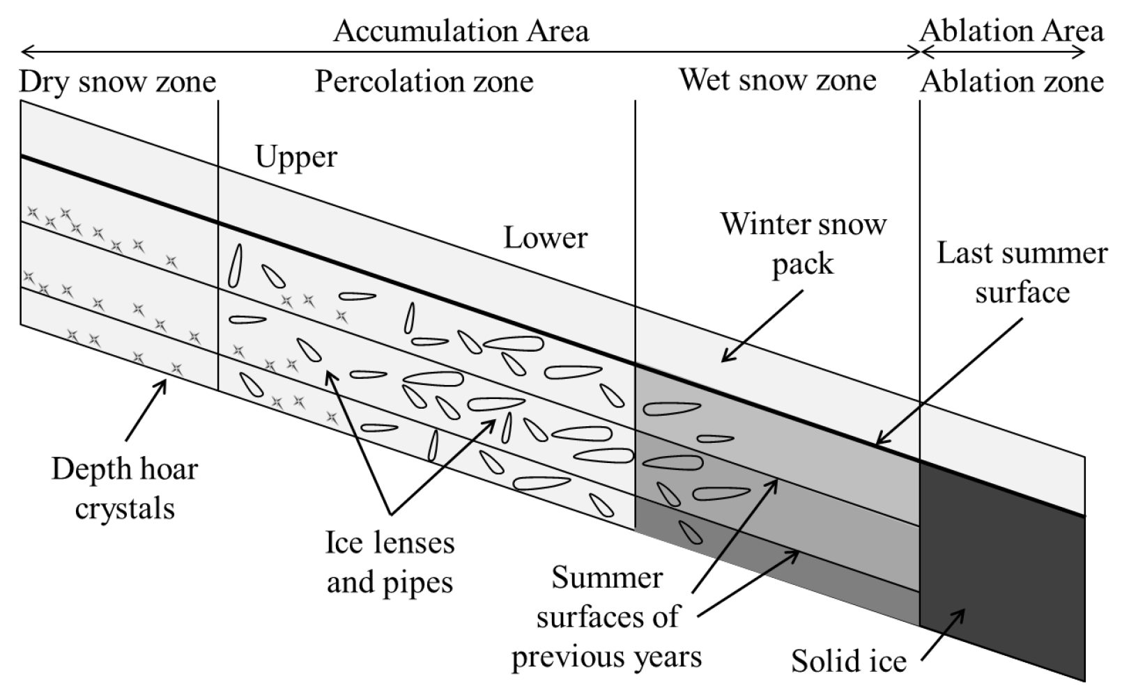
2] divided the Ice Sheet into four zones, according to
Figure 1. Melt does not occur in the dry snow zone, which is situated at the highest altitudes at the center of the Greenland plateau. The snow is gradually compacted under its own weight and the surface layer is subject to modifications due to wind effects. Moreover, the properties of the dry snow zone are not uniform, since it is characterized by different levels of snow accumulations, systematically decreasing from the southwest to the northeast regions of Greenland [
3,
4]. This inner region is surrounded by the percolation zone, where a limited amount of melt per year occurs, leading to the generation of larger snow grains and to the formation of small ice structures, like lenses and pipes, within the snow pack. The size of such ice formations can vary from some centimeters to tens of centimeters [
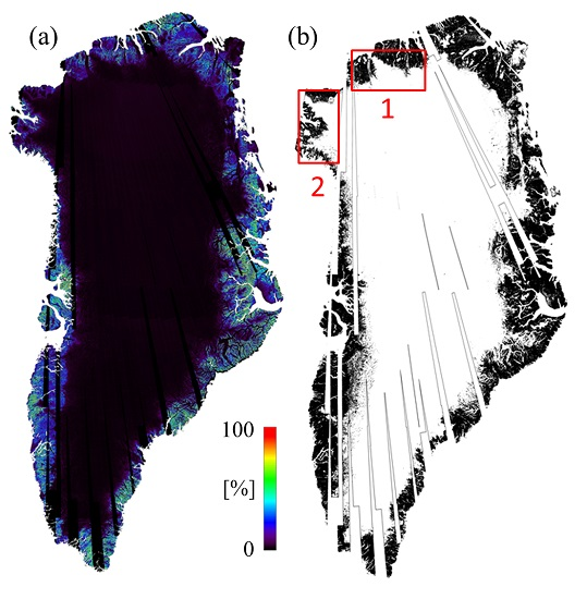
5]. The wet snow zone is located further down slope towards Greenland’s coasts, where a substantial part of the snow melt drains off during summer, and is characterized by the presence of multiple ice layers. Outer coastal regions are finally classified as ablation zone, where the previous year accumulation completely melts during summer, resulting in a surface of bare ice and surface moraine. Up to now, the different facies have been located using microwave sensors by estimating the backscatter levels of the reflected signal [
6,
7]. The dry snow zone is characterized by low levels of backscatter, given the absorption of the incident radar wave; on the other hand, the presence of ice pipes and lenses in the percolation snow, whose dimensions are comparable to the wavelength of the incident radar wave, strongly increase the backscattered signal from such a region. The scattering mechanisms occurring in the wet snow zone are similar to those in the percolation zone, even though a higher variability is expected during summer, due to increased melt rates [
5]. Moreover, the availability of several spaceborne SAR missions allows for the monitoring of radar backscatter evolution in time, demonstrating the great potential of radar to track down changes in the Ice Sheet properties [
8].
The penetration of an incident radar wave on a snow pack is dependent on the sensor’s frequency and wave polarization, and on the characteristics of the illuminated target, such as snow density and structure, leading to volume scattering. Interferometric synthetic aperture radar (SAR) acquisitions over the Greenland Ice Sheet are therefore subjected to volume decorrelation [
9]. Its amount can be associated to the dominant backscattering mechanism for radar waves incident onto a snow pack, helping to classify the characteristics and structure of the snow pack itself.
The German SAR mission TanDEM-X has the primary goal of generating a global, high-precision digital elevation model (DEM) with a spatial resolution of 12 m [
10,
11,
12]. Since October 2010, two twin satellites TerraSAR-X and TanDEM-X have been flying in a close orbit configuration, acting as an X-band single-pass SAR interferometer and systematically scanning the Earth’s land masses in bistatic single horizontal polarization stripmap mode, with a swath width of about 30 km. In this paper we present an approach to locate and investigate different snow facies by exploiting TanDEM-X interferometric SAR acquisitions over the snow-covered areas of Greenland. TanDEM-X data, acquired in X-band at 9.6 GHz, are particularly suitable for this analysis due to the single-pass bistatic capabilities of the system, which does not suffer from temporal decorrelation [
13]. As far as spaceborne SAR sensors are concerned, this data set is unique.
The goal of classification techniques is to group together the input data in different classes on the basis of a defined measure of similarity. The approach can either be supervised, if a priori knowledge is introduced for defining the properties of the different classes, or unsupervised, if such classes are directly estimated from the input data, without external additional information. Since only a few local studies have been performed for determining the properties of the Greenland and Antarctica Ice Sheets using X-band SAR data [
14,
15,
16], only a limited a priori knowledge is available for directly defining the characteristics of each snow facies from X-band signatures. Unsupervised classification techniques, such as fuzzy clustering, therefore represent an attractive technique.
A first preliminary study on the potential of TanDEM-X interferometric data for snow facies analysis using fuzzy clustering was presented in [
17]. We refined the classification algorithm, investigated its performance in detail, and performed comparisons with in situ observations to support interpretation of the results. In
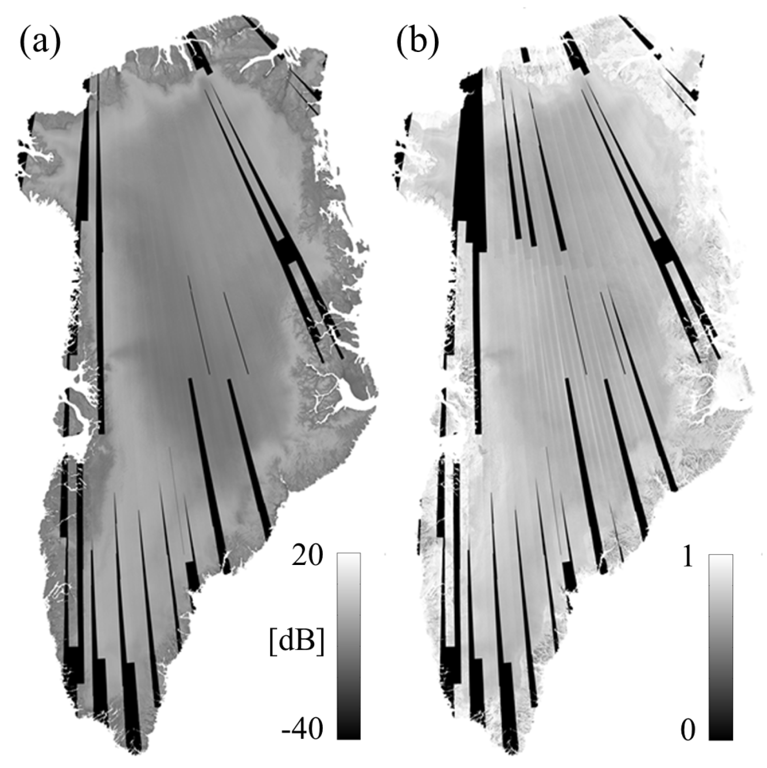
Section 3 we describe the large-scale mosaics of SAR backscatter and volume correlation factor, together with additional parameters, derived from systematic TanDEM-X interferometric acquisitions. These mosaics are the starting point for applying the
c-means fuzzy clustering algorithm, detailed in
Section 2.1. We present the obtained results in
Section 4, where we also address the use of different number of clusters. Their interpretation is discussed in
Section 5, by means of reference melt data, snow density, and in situ measurements of snow structure. A dedicated sub-clustering of the inner snow facies allows to further refine its classification, as discussed in
Section 5.3. In
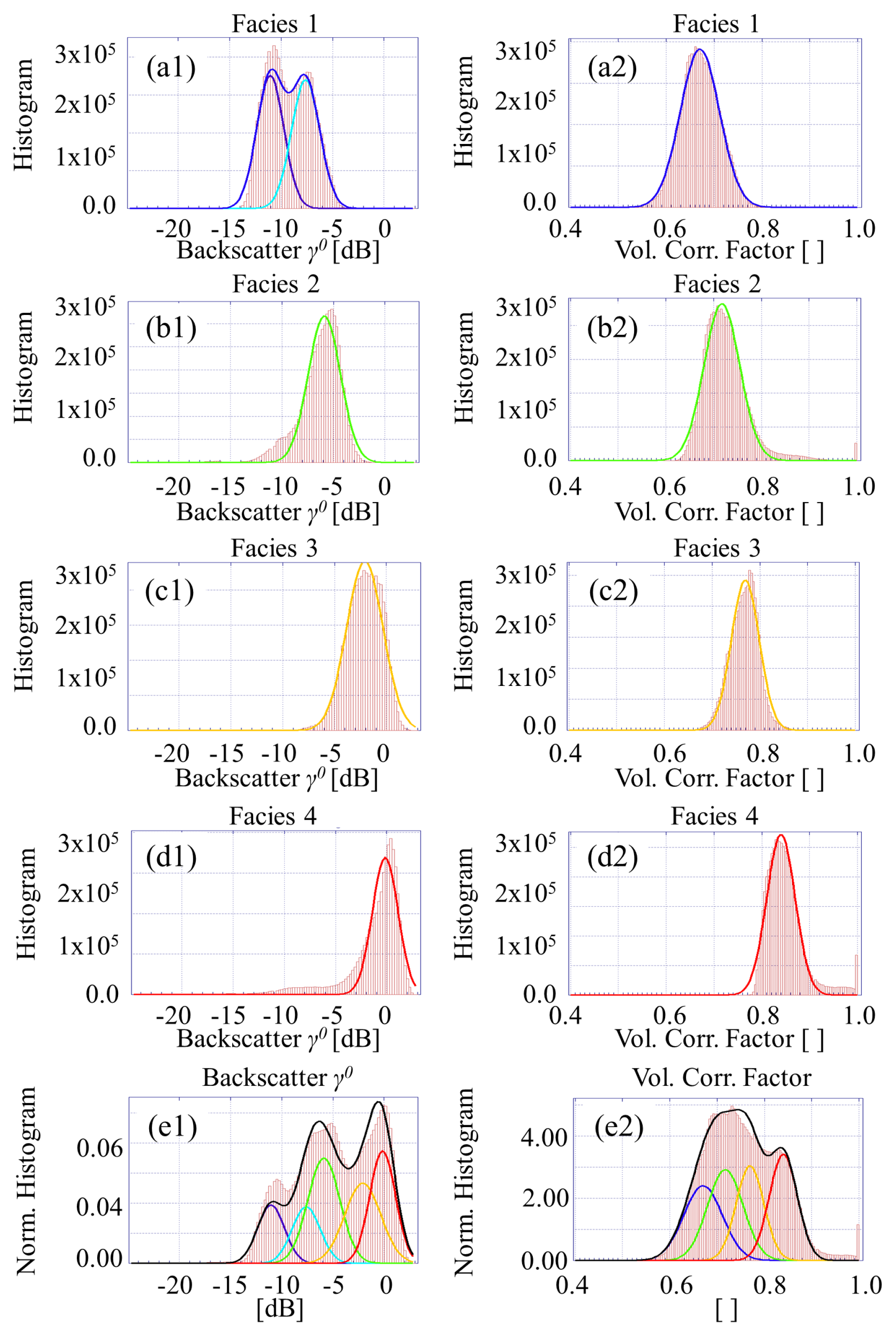
Section 5.4, we present a statistical analysis of backscatter and volume decorrelation for the derived snow facies, which allows to fit a Gaussian model to the histograms of these quantities. Finally, knowing the location of the different facies, it is possible to estimate the X-band penetration depth along the whole Ice Sheet, as explained in
Section 6, and to compare it to an independent estimation, obtained by composing TanDEM-X digital elevation model (DEM) data and ICESat laser altimeter measurements. Conclusions are finally drawn in
Section 7.
2. Fuzzy Clustering for Snow Facies Classification
In this section we describe the method used to classify the different snow facies of the Greenland Ice Sheet. It is based on the use of the
c-means fuzzy clustering algorithm, developed by J. Bezdek et al. in [
18], which is an unsupervised classification algorithm based on fuzzy logic theory.
In this work, two characterizing radar quantities are considered for classifying snow facies: radar backscatter and coherence contribution due to volume decorrelation. The choice of an unsupervised classification method resides in the fact that a gradual transition of backscattering intensity between different snow facies on the Greenland Ice Sheet was observed by K. C. Partington in [
19], impairing the use of a manual partitioning approach, which would strongly depend on the subjective choice of the decision thresholds. Moreover, the
c-means fuzzy clustering algorithm has already been used in the literature for discriminating snow facies using Envisat active and passive microwave observations, showing it to be a promising approach for clustering similar regions of the Greenland Ice Sheet, as presented by Tran et al. in [
20].
2.1. The Fuzzy c-Means Clustering Optimization
Clustering defines the task of grouping together elements coming from an input set of observations, depending on how similar they are to each other. The observations are divided into
c non-empty subsets called clusters. Since in reality clusters may show some kind of overlap, fuzzy-clustering has been introduced [
21]. The fuzzy
c-means clustering algorithm is an iterative optimization algorithm which allows the determination of the optimal cluster centers without requiring a priori information [
22]. In literature, the fuzzy
c-means clustering has been found to be very popular within the research community, being used for a large variety of applications, such as risk and claim classification or vehicular pollution estimation [
23,
24].
The idea is to represent the similarity that an observation shares with each cluster by using a membership function, whose values are between 0 (0% probability of belonging to cluster i) and 1 (100% probability of belonging to cluster i). The results are fuzzy c-partitions of the input observation data set, which contain observations characterized by a high intracluster similarity and a low extracluster one.
For a given input vector of N observations, defined as (), where each is characterized by P features, the membership function can be expressed using a real matrix . The cluster center is then identified by a P-dimensional tie-point vector .
If cluster centers are not known by
a priori considerations, an optimization method has to be applied in order to estimate them. Their locations are iteratively determined by optimizing the following objective function:
where
is the squared Euclidean distance from point
to the cluster center
. The parameter
m controls the fuzziness of the algorithm:
produces hard partitions of
, while increasing
m allows the single clusters to overlap, blurring the membership degree to higher levels of fuzziness. Since the Euclidean distances of the observations from the cluster centers in Equation (
1) have to be minimized, it is important to scale the different features to the same order of magnitude, in order to avoid having a predominant one, which would affect the classification accuracy. In this work, we decided to normalize each input set of features to a unit standard deviation as:
where
is a vector containing the
N input values of
for the
feature and
is the standard deviation.
By substituting the normalized input data set
into (
1), the optimal clustering of
is therefore obtained as:
and
can be optimized by iterating over the following equations:
After a random initialization of
, (
4) and (
5) are iteratively updated until convergence is obtained. A convergence test can be performed by computing the mean square error between
at steps
and
.
A recurrent issue of the c-means clustering algorithm is to remain stuck in a local minimum, being unable to provide a meaningful set of cluster centers. A proper initialization of the cluster centers is therefore highly recommended, as presented in the next section.
2.2. Algorithm Initialization
The algorithm initialization represents a crucial step in avoiding local minima. Many investigations have been carried out on finding an effective initialization for the algorithm; in this paper we based our initialization on the work presented in [
25]. The input set of normalized observations per feature
is transformed into a positive vector
by:
Now the Euclidean distances of each scaled observation from the origin are evaluated and sorted in increasing order. The corresponding scaled observations are sorted accordingly. Given the desired number of output clusters c, the sorted observations are grouped together into c subsequent sub-sets, each of those composed of observations. For each sub-set, a cluster center is then initialized by evaluating, for each feature, the mean value of all available observations.
4. Classification Results
In this section we present the results obtained by applying the classification method, described in
Section 2, to the input data set of interferometric TanDEM-X acquisitions, presented in
Section 3. We selected
features, namely
and
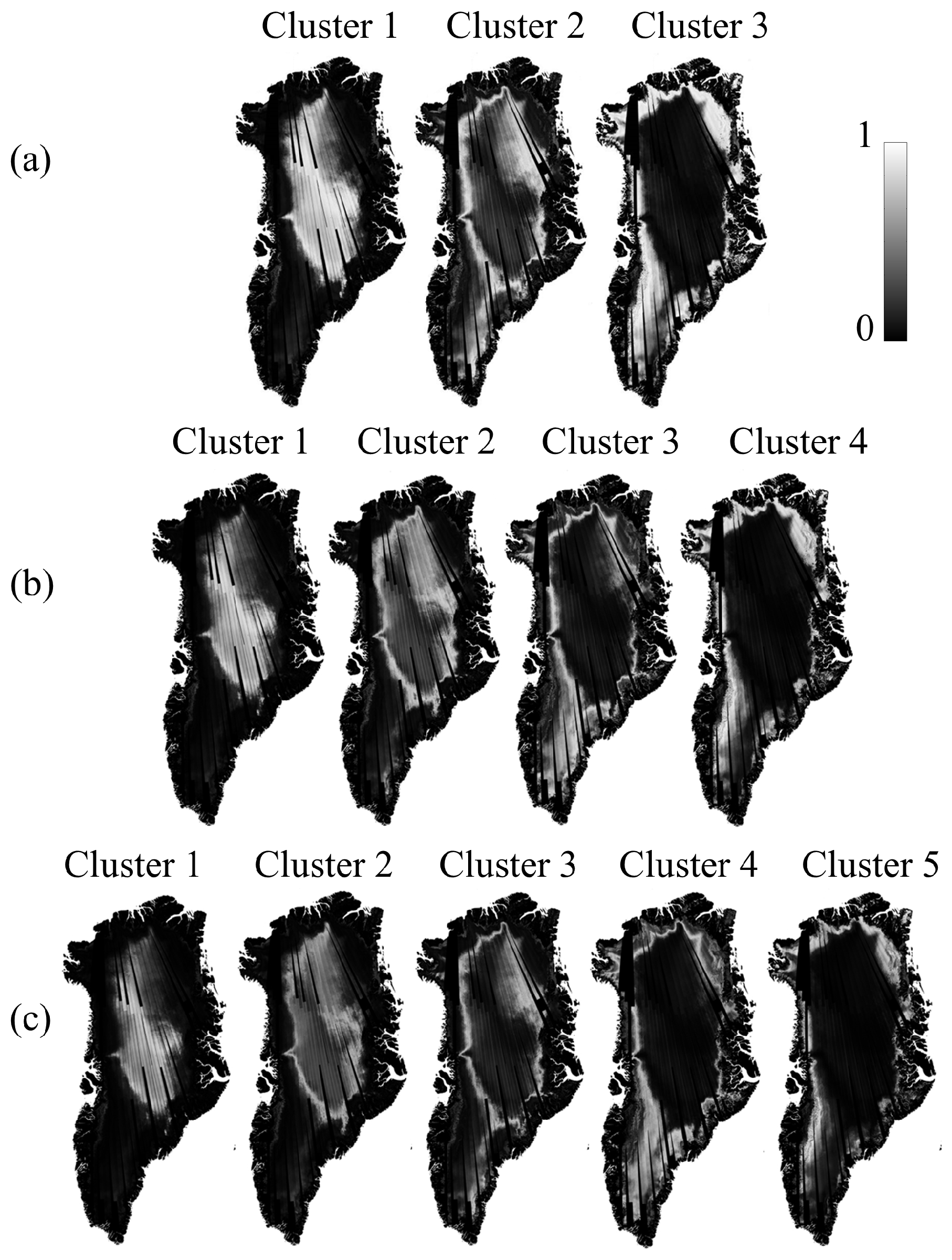
, and tested different numbers of clusters. We report here the results obtained using
number of clusters. The
m parameter was set to 2. The resulting membership maps are displayed in
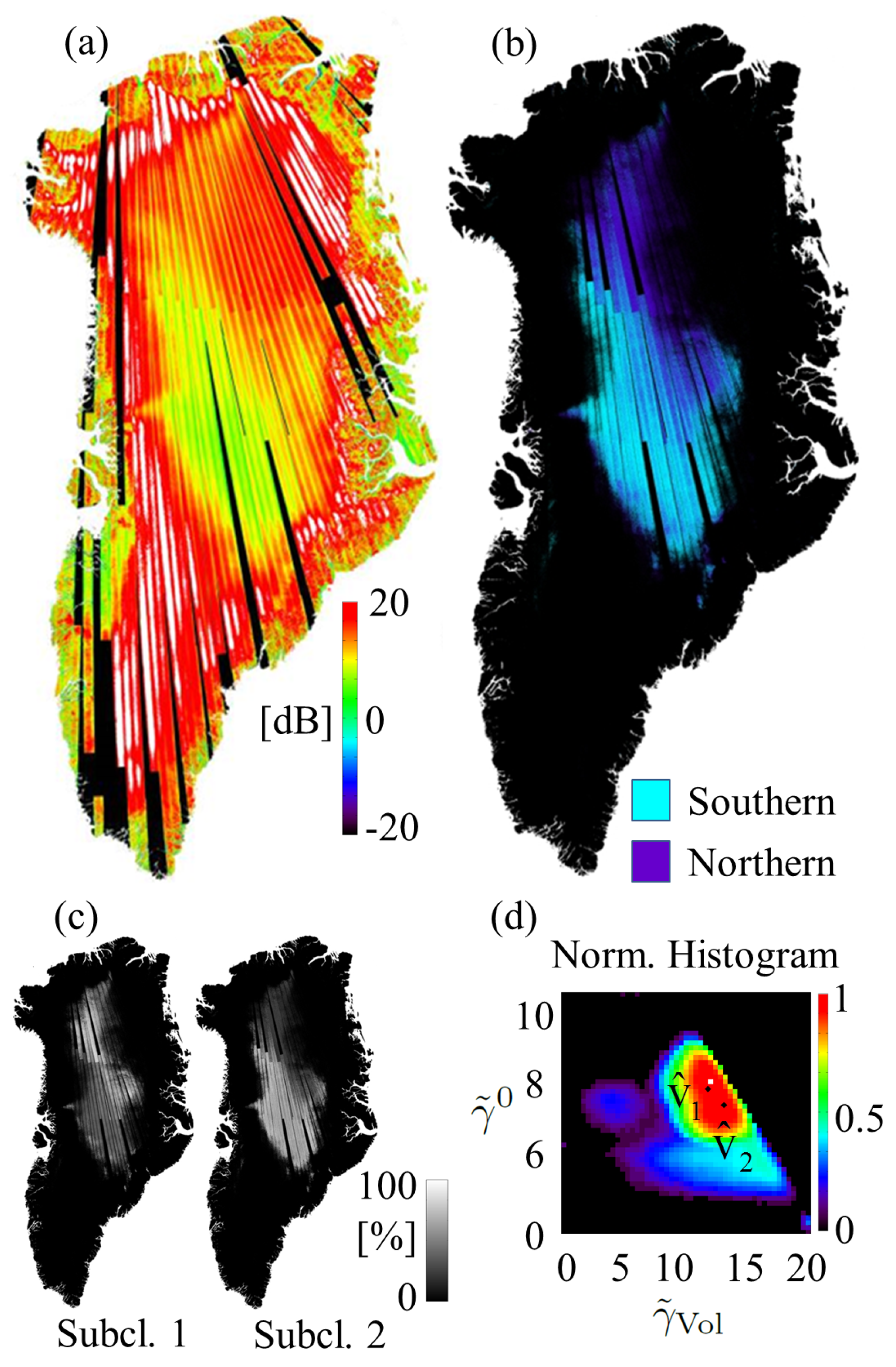
Figure 6. A high percentage corresponds to a high probability of belonging to a specific cluster. The classification results for the three different sets of clusters are presented in
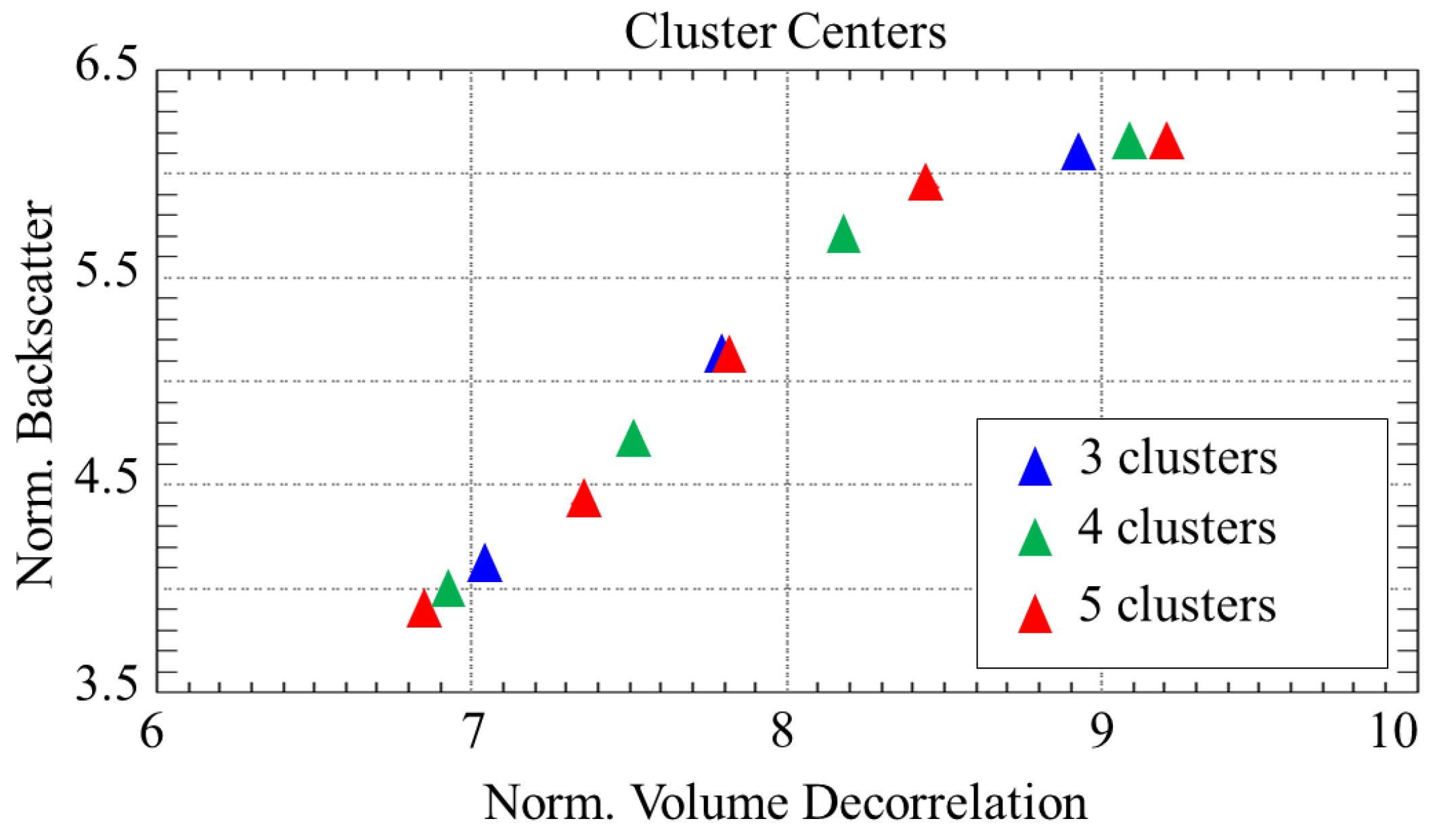
Figure 7a–c. The corresponding normalized histograms of the input data, together with the location of the cluster centers
, are depicted in
Figure 7d–f, where the horizontal and vertical axis display the normalized volume correlation factor
and the normalized backscatter
, evaluated as:
being
and
the standard deviations of
and
, respectively. For the considered input data set, we have
,
,
dB, and
dB. The cluster centers for the selected partition in the normalized histogram of the input data are given in
Figure 8.
The fuzzy partition of three clusters shows a higher distance among the single cluster centers. Higher numbers of clusters are also characterized by a higher degree of inter-cluster overlap and result in a classification where lower values of the membership matrix are accepted for associating a certain cluster to an input observation. Nevertheless, increasing the number of clusters allows to get a more detailed characterization of the different snow facies, strongly influenced by increasing melt phenomena from the center of the plateau toward the outer edges.
The algorithm was run using a higher a-priori number of clusters
c as well, obtaining partitions characterized by a very limited extend and increasing the confusion between adjacent classes. Such a trend is already visible when using
(
Figure 7c), where cluster 2 (light blue) corresponds to a very thin intermediate layer between cluster 1 (blue) and cluster 3 (green) and is entirely characterized by the presence of pixels classified as both cluster 1 and 3. This trend is maintained for higher number of cluster centers and the results are here omitted.
Furthermore, for the three different numbers of selected clusters presented in
Figure 7, the percentage of pixels classified accordingly to a membership value which is higher than 0.3, 0.5, 0.7 and 0.9 are summarized in
Table 1. The results indicate that, using four clusters, over 81% of the pixels are classified with a membership value above 0.5. From a pure algorithmic point of view, such a partition shows therefore a reasonably good performance in terms of classification reliability.
Based on this finding, we decided to consider the partition with
for our further investigation, which represents a good trade-off between a satisfying level of detail and a good separation between adjacent clusters. From now on, we will therefore refer to snow facies instead of clusters and we will consider the map presented in
Figure 7b as reference, characterized by the presence of 4 different snow facies.
Finally, by considering an overall Ice Sheet surface of 1,700,000
, it is possible to estimate the extension of each snow facies. The results are presented in
Table 2.
6. Estimation of the Penetration Depth
Knowing the properties and the location of the different facies of the Greenland Ice Sheet represents the bases for further scientific investigations. In this section, we derive a map of the penetration depth, based on the model presented by Weber Hoen and Zebker in [
9] and we compare it to real elevation measurements from TanDEM-X data. By assuming a homogeneous, lossy scattering medium, they modeled the volume correlation factor
with respect to the one-way power penetration depth
as:
where
is the dielectric constant and, for an icy medium, it is supposed to be real and to remain constant throughout it.
represents the penetration depth where the one-way power decreases by
. By inverting (
17), we obtain
as:
The two-way penetration depth
can then be derived as:
We consider the two-way penetration depth because it is the one that approximates the location of the radar mean phase center and is therefore related to the measured interferometric height.
By exploiting the snow facies map in
Figure 9a, we can now associate to facies with a proper value of
. The dielectric constant
can be related to the snow density
as presented in [
43]; taking the single measurements which relate the density to the permittivity in H polarization, we performed a 2nd-order polynomial fitting, shown in
Figure 14. Assuming a homogenous density of snow within the most superficial layers of the snow pack (until about 10 m depth), the mean snow density
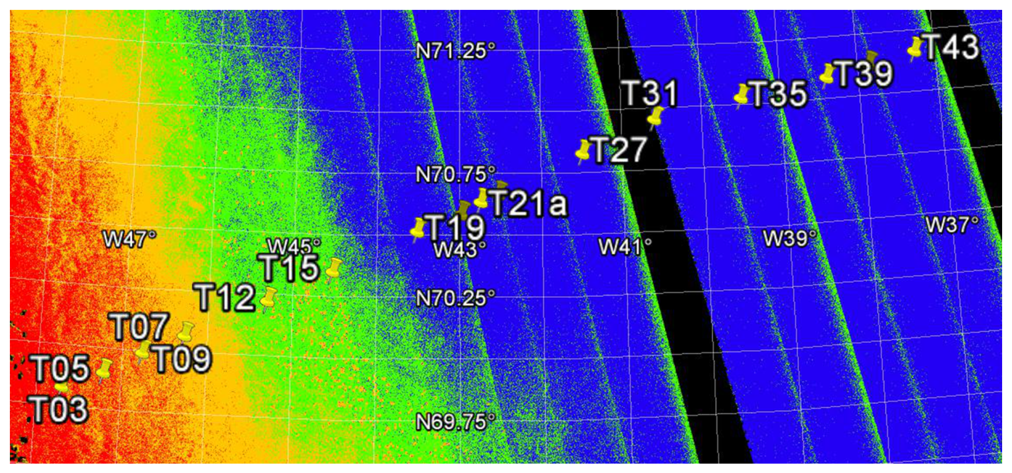
along the EGIG line, accumulated over the period of spring 2004 to summer 2006, can be extrapolated from Equation (20) in [
40] and associated to the different test sites, depending on the distance from T05 (as in Table 1 of [
40]), leading to the following values:
at T05 (belonging to facies 4): ,
at T09 (belonging to facies 3): ,
at T12 and T15 (belonging to facies 2): and ,
from T21 to the summit of the traverse (belonging to facies 1): decreases from about to about .
When more than a single
value per facies are available, the mean value has been considered. These values are summarized in
Table 5, together with the corresponding permittivities. By substituting the derived
into Equations (
18) and (
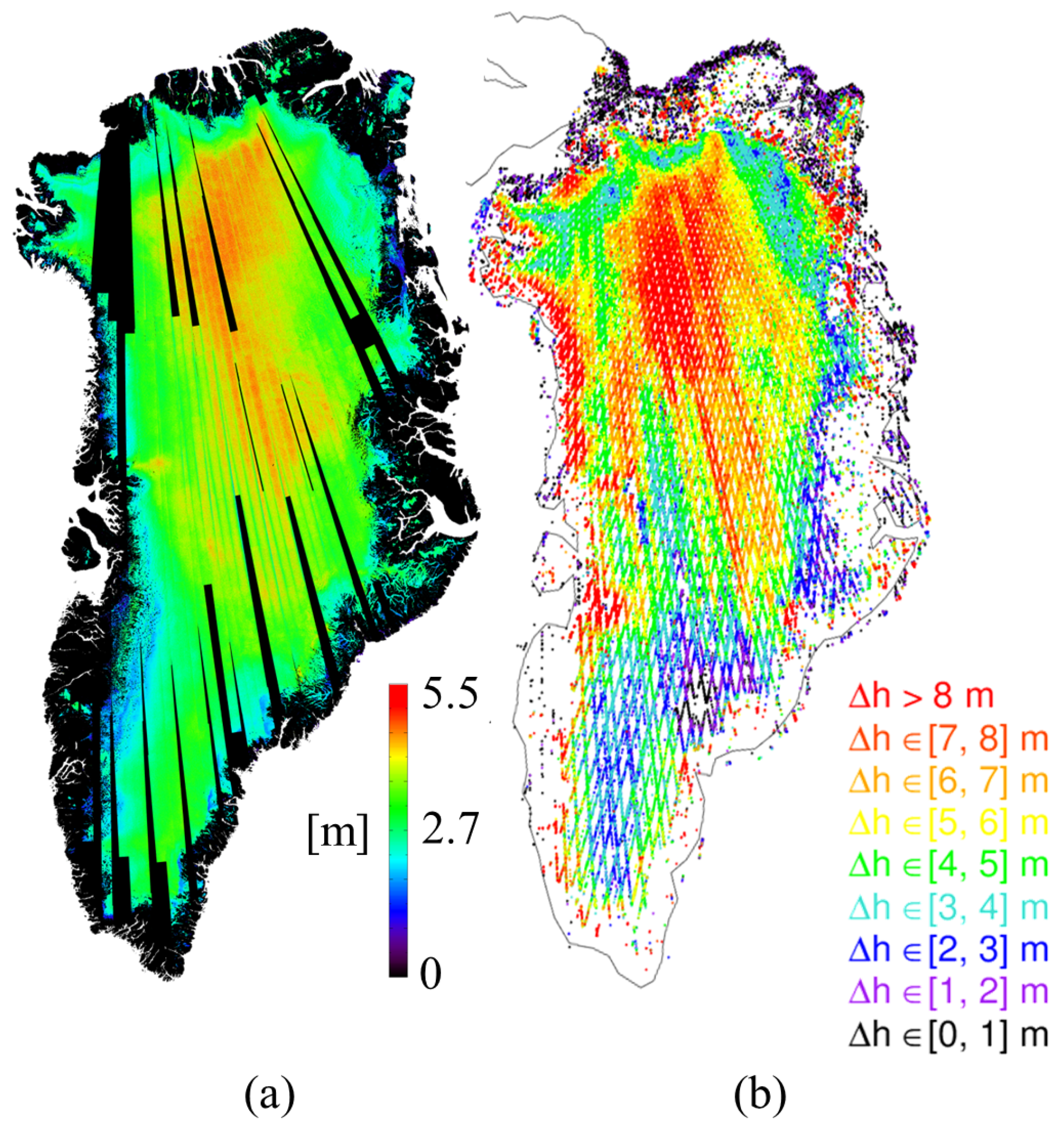
19), together with the other parameters derived for the considered TanDEM-X acquisitions, we obtain the map of the two-way penetration depth in
Figure 15a. The corresponding histograms for each facies are depicted in
Figure 16a and the mean value
and standard deviation
for each distribution are summarized in
Table 6.
The obtained results over facies 1 (characterized by dry snow) match very well with the ones obtained by Rott et al. in [
14], where a one-way penetration depth of 8.1 m at 10 GHz was estimated for dry, highly metamorphic snow, corresponding to a two-way penetration depth of 4.05 m.
We also compared the obtained results to the difference between ICESat laser elevation measurements, carried out between 2003 and 2009 [
44], and the final global TanDEM-X DEM. As already mentioned, radar DEMs typically represent the location of the mean phase center of the backscattered signal; in case of penetration into the snow pack, they will differ from ICESat, which measures the height of the surface. For each available ICESat value, we evaluated the mean difference
between ICESat and TanDEM-X DEM as:
where
identifies the mean height of the final TanDEM-X DEM within the considered ICESat footprint and
represents the measured height from ICESat over the same ground area. The results are shown in
Figure 15b.
has been separately evaluated for the four different snow facies in
Figure 9a by applying a defined polygon for each zone, derived as presented in
Figure 9. The corresponding histograms for the different facies are depicted in
Figure 16b and the mean values and standard deviations are again summarized in
Table 6. It has to be mentioned that ICESat measurements are older than the considered TanDEM-X DEMs. In the time intermediate there have been changes in the height of the Ice Sheet that introduce a further amount of uncertainty in the estimation.
The depth of the mean phase center of a radar wave, measured by the interferometric phase, approximately equals the two-way penetration depth
if the latter is lower than about 10% of the height of ambiguity
, otherwise a bias between the two is introduced [
45]. For the current analysis, the worst-case can be estimated using the ratio between the
two-way penetration depth over the dry snow zone, given by
m, and a minimum
of about 40 m (
Figure 13). The result is a ratio of about 14%, which allows us to reasonably assume that no significant bias is introduced between the two-way penetration depth
and the elevation measurement
.
We can now evaluate the difference
between the mean
and the mean
for each snow facies as:
Assuming a good accuracy of the two-way penetration depth
, at least confirmed for the inner snow facies (characterized by the presence of dry snow) by the results obtained by Rott et al. in [
14],
is expected to be around zero. Even though the results match quite well, the obtained values, shown in
Table 6, indicate the presence of a slightly negative offset which varies from about −0.8 m to −1.4 m.
A reason to at least partly explain such differences is the simplified (single layer) model of Hoen and Zebker for relating volume decorrelation to penetration depth. The model assumes that there is no depth dependency of the scattering cross-section, a constant density, and uncorrelated scatterers. This hypothesis is not true for a highly stratified medium such as polar firn, as addressed in
Section 5.2 [
39,
40]. For example, since the penetration depth at X-band is on the order of a few meters, the density of the upper layers of the snow pack becomes of predominant importance. In particular, the first two meters typically present lower density than the mean values used here (see e.g., Figures 2 and 5 in [
40]). If we now assume a decrease of
in snow density, which is comparable to the density change in the upper layers in [
39,
40] with respect to the mean one, this would result in an increase of the mean two-way penetration depth in the range from 7 cm (facies 1) up to 17 cm (facies 4), reducing the remaining offsets by the same amount.
Other sources of uncertainty may result from the fact that the TanDEM-X DEM has been calibrated using ICESat measurements in the outer regions of Greenland only. Along the Ice Sheet a self-adjusting block calibration has been implemented [
46], which might also explain the persistence of a residual offset. A further reason might be the occurrence of height changes during the time span which separates ICESat measurements from TanDEM-X acquisitions.
A way to improve the accuracy of the penetration depth model could be to combine both backscatter and volume decorrelation information, which would be consistent with the applied snow facies classification method, which considers both quantities. This topic will be the object of further investigations.
7. Summary and Conclusions
In this paper we present an approach for locating different snow facies of the Greenland Ice Sheet by exploiting X-band TanDEM-X interferometric SAR acquisitions. We applied an unsupervised classification method based on the c-means fuzzy clustering algorithm, which uses features inherent in the data without subjective interference. This is an appropriate method for exploring the information content of the 2D feature space, given by the combination of radar backscatter and volume correlation factor , with respect to glacier facies, which is a main objective of the work. The algorithm has been applied to TanDEM-X data acquired during winter 2010/2011, by analyzing three different partitions, obtained by selecting a different number of clusters (), in order to assess the feasibility for discriminating facies types. The partition composed of 4 clusters is a good compromise in terms of classification reliability and high level of detail and has therefore been chosen as reference for the current work. We then provided a statistical analysis of both and over the Ice Sheet for each different facies and investigated the dependency of on the acquisition geometry and, in particular, on the height of ambiguity ranging from 40 m to 53 m. The use of a correction factor for depending on the height of ambiguity might represent a starting point for a future refinement of the classification algorithm.
The derived snow facies have been interpreted by means of reference melt data and in situ measurements along the EGIG line.
Facies 1 is dominated by the presence of dry snow. Further refined clustering reveals two sub-facies (a southern and a northern one) which can be related to different snow accumulation rates. Facies 2 to 4 belong to a transition zone where melt phenomena increase toward the outer regions of the Ice Sheet. Facies 2 and 3 approximately correspond to the percolation zone, and facies 4 to the wet snow zone, reported by Benson in [
2]. This is confirmed by structural properties of the snow volume as observed by Morris and Wingham in [
40]. The subdivision into different facies results from differences in
and
due to spatial changes in microstructure of firn related to melt intensity and accumulation rates, which vary with elevation, snowfall pattern, and wind drift. The subdivision is therefore a pointer to such differences.
Given the high similarity in terms of backscattering properties and volume decorrelation among pixels belonging to the same cluster, we can then apply the mean value of snow density to the entire considered snow facies. This allowed us to estimate the penetration depth by inverting the interferometric model proposed by Weber Hoen and Zebker in [
9] and assuming the dielectric constant for an icy medium to be real and to remain constant for a given facies type. The obtained results show a mean two-way penetration depth of 4.18 m for facies 1, 3.58 m for facies 2, 3.07 m for facies 3, and 2.34 m for facies 4. These values have been compared to the elevation between the global TanDEM-X DEM and ICESat measurements, proving that, theoretically, no considerable bias between the two measurement approaches is to be expected. A residual negative offset has nevertheless been detected, which varies from about −0.8 m to −1.40 m for the different snow facies, which will be object of further investigations. A possible explanation might be the fact that the Weber Hoen and Zebker’s model relies on simplifying assumptions, such as no depth dependency of the scattering cross-section, a constant density, and uncorrelated scatterers. Other sources of uncertainty may be related to the TanDEM-X DEM calibration or to the occurrence of height changes during the time span which separates ICESat measurements from TanDEM-X acquisitions.
Even though featuring a limited penetration into the snow pack, TanDEM-X interferometric data demonstrates itself to be highly sensitive to changes in snow properties and represents a highly valuable data set for investigating Greenland Ice Sheet characteristics and its evolution. The continuous monitoring of the cryosphere in an era of climate changes represents one of the most challenging tasks for the remote sensing community. The developed approach can also be applied to more recent TanDEM-X acquisitions over Greenland and Antarctica Ice Sheets, to characterize their properties and changes. The work performed here represents therefore a starting point for further analyzing the evolution in time of Ice Sheets, by monitoring the changes in the location of the different snow facies, as an indicator of climate changes. Moreover, the technique could be exploited within future interferometric SAR missions as well. For example, the Tandem-L mission is being currently designed for acting as single-pass interferometer at L-band [
47], with the main object of assessing the dynamic processes in the Earth’s environmental system.


