Article

Sea Ice Concentration Estimation during Freeze-Up from SAR Imagery Using a Convolutional Neural Network

Department of Systems Design Engineering, University of Waterloo, Waterloo, ON N2L 3G1, Canada
*
Author to whom correspondence should be addressed.
Remote Sens. 2017, 9(5), 408; https://doi.org/10.3390/rs9050408
Submission received: 27 January 2017 / Revised: 17 April 2017 / Accepted: 21 April 2017 / Published: 26 April 2017
(This article belongs to the Special Issue Learning to Understand Remote Sensing Images)

Abstract

:
In this study, a convolutional neural network (CNN) is used to estimate sea ice concentration using synthetic aperture radar (SAR) scenes acquired during freeze-up in the Gulf of St. Lawrence on the east coast of Canada. The ice concentration estimates from the CNN are compared to those from a neural network (multi-layer perceptron or MLP) that uses hand-crafted features as input and a single layer of hidden nodes. The CNN is found to be less sensitive to pixel level details than the MLP and produces ice concentration that is less noisy and in closer agreement with that from image analysis charts. This is due to the multi-layer (deep) structure of the CNN, which enables abstract image features to be learned. The CNN ice concentration is also compared with ice concentration estimated from passive microwave brightness temperature data using the ARTIST sea ice (ASI) algorithm. The bias and RMS of the difference between the ice concentration from the CNN and that from image analysis charts is reduced as compared to that from either the MLP or ASI algorithm. Additional results demonstrate the impact of varying the input patch size, varying the number of CNN layers, and including the incidence angle as an additional input.

Graphical Abstract

1. Introduction

In the operational sea ice community, visual analyses of SAR imagery by expert ice analysts are a key contribution to ice charts, which are used to assist navigation and operations in ice-covered waters [1]. However, the generation of these analyses is time consuming. Upcoming and new satellite missions, such as the Canadian RADARSAT Constellation Mission (RCM), and the European Sentinel mission, will lead to significantly increased volumes of SAR imagery [2], increasing the need for automated methods to analyze the imagery.
There are several previous studies extracting information from SAR imagery using automated methods. Many of these studies use ‘engineered’ or hand-crafted features, which are features designed and selected to carry out a specific task. Examples include, the HH autocorrelation, normalized polarization difference and cross-polarization ratio all of which have been used in ice concentration estimation [3,4], grey level co-occurrence matrix features, Gabor filters and Markov random fields, which have been used to classify imagery into ice type and ice/water [5,6,7,8], and curvelet features used to locate the ice edge [9]. One of the challenges with using a set of engineered features to automatically extract information from SAR imagery is the difficulty of developing a set of robust features that can be applied to different geographic regions and seasons and for different imaging geometries. To capture various ice conditions, features may need to be designed for different locations or times of the year. For example, a large database of HH and HV backscatter values that represent typical signatures of 100% ice cover has been generated to retrieve ice observations for use in data assimilation. In the database, the backscatter values are estimated for each month as a function of incidence angle and windspeed on a region dependent-basis [10]. Such an extensive database may be necessary to assess the robustness of engineered features for large-scale applications, such as estimating ice concentration for assimilation in an operational prediction system [11]. Data assimilation requires high quality observations due to the nature of the assimilation cycle, in which erroneous observations will lead to an erroneous analysis, the influence of which will persist when the analysis is used to initialize the next assimilation cycle. For example, the open water regions that are estimated by Karvonen [4] as having an ice concentration of 10% or 15% would generate an incorrect analysis in a sea ice data assimilation system. A similar situation would arise upon assimilating a consolidated ice cover estimated with passive microwave data, in the event that the real ice cover has cracks and leads. Such openings in the ice are crucial for heat transfer from the ocean to the atmosphere. When the ice cover is used as a boundary condition for numerical weather prediction, an accurate estimate of the sea ice concentration is critical [12].
When an analyst estimates ice concentration from a SAR image, they combine their knowledge of ice conditions in the region with visual cues in the image. This may involve looking at the SAR image features over a range of scales. For example, at large scale, tonal changes across a region can be used to identify the region as either ice or open water, while at small scale visible ridges in the ice cover may indicate a region of high ice concentration, or small-scale ice floes may indicate a marginal ice zone. Thus, if it is desired to emulate the analyst’s task, the goal can be viewed as emulating the human visual system’s ability to assimilate information at various scales with prior knowledge. Convolutional neural networks (CNNs) are a known method to learn features from images, taking into account information at various scales. The training takes place by minimizing a difference between output of the CNN and training data, which represents prior knowledge. Remarkable similarities between CNNs and the human visual system have been demonstrated in numerous studies [13].
The present study uses a CNN trained with image analysis charts to estimate ice concentration from SAR imagery acquired over the Gulf of St. Lawrence during freeze-up in the winter of 2014. A previous study [14] has evaluated a similar architecture for the problem of ice concentration estimation in the Beaufort Sea for the 2010-2011 melt period. The present study builds on that work, addressing the following questions: (i) Can a CNN estimate sea ice concentration accurately during freeze-up, when the ice is very thin and may be difficult to distinguish from open water [15,16]? (ii) How is the performance of the CNN affected when some of the parameters (e.g., number of layers and input patch size) are modified? (iii) Can a CNN manage to interpret ice concentration for environments, such as the Gulf of St. Lawrence, where the ice characteristics are dynamic?

2. Background

Learning image features from SAR imagery to estimate ice concentration, as compared to first calculating engineered features from the image, builds on previous work in feature learning, which is a promising method to analyze complex and large volumes of data [17,18,19,20,21]. Deep learning is a type of feature learning method that can automatically extract complex data representations at high levels of abstraction [18,22,23]. For image recognition tasks, deep convolutional neural networks (CNN) are widely used due to their ability to model local image structures at multiple scales efficiently [24,25,26,27].
There has been limited research in using CNNs to learn features from satellite images. Related studies include using CNNs for road classification from aerial images [28] and the detection of vehicles [29] and buildings [30] from high resolution satellite images. Training of CNN models requires a large quantity of high quality training samples. For many remote sensing problems, gathering high quality ground truth is expensive and sometimes not feasible, due to the vast study area and diversity of surface conditions. This is in particular the case for ice concentration mapping. Due to harsh environmental conditions and in the interest of safety, obtaining adequate in situ samples coincident or near-coincident in time with a SAR scene is not usually feasible. Normally such in-situ studies are limited to small geographic regions and a limited time period.
Using other sources of satellite data or output from ice-ocean models may not be very suitable choices for training data. For example, many algorithms that compute ice concentration from passive microwave data are known to be biased over thin ice and in regions with low ice concentration levels [16,31,32]. Training a CNN with this data will lead to a CNN model that generates similar biases. Ice concentration estimated by image analysts is considered the best available ice concentration information [33]. Hence, the extensive image analysis database at the Canadian Ice Service (CIS) represents a promising archive that can be used to provide data to investigate the use of a CNN to estimate ice concentration from SAR imagery.

3. Data and Study Area

The study area is located in the Gulf of Saint Lawrence, which is situated on the east coast of Canada (Figure 1). The period of study extends from 17 January 2014 to 10 February 2014. This time of year corresponds to freeze-up in the Gulf of Saint Lawrence, with both ice concentration and thickness increasing from January into February. For the duration of the study, the ice cover is composed of new ice (less than 10 cm in thickness) and grey and grey-white ice (10–30 cm in thickness), with thicker first-year ice near Prince Edward Island. Definitions for the various ice types are provided by the World Meteorological Organization (WMO) [34].
A total of 25 RADARSAT-2 dual-pol (HH and HV) ScanSAR Wide [35] images are used for the present study. The full list of the SAR images used is provided in Table 1. The nominal pixel spacing of the acquired SAR images is 50 m by 50 m, and the incidence angle ranges from 20 to 49 . The image size is roughly 10 k × 10 k covering a spatial extent of about 500 km × 500 km. The outlines of all the SAR images in the dataset are shown in Figure 1.
Each SAR image has an accompanying image analysis chart, which is used to provide the training data to the ice concentration estimation methods. Compared to other types of ice charts (daily ice chart and regional ice chart), image analysis charts provide a more detailed interpretation of SAR images and are valid at the SAR image acquisition time [34]. Image analyses are prepared manually by a trained analyst who identifies regions (polygons) in which the ice conditions appear to be uniform, in terms of the total ice concentration and the relative mix of ice types. The ice types are defined according to their stage of development following World Meteorological Organization standards [34]. The ice concentration label given to a polygon is assigned in increments of 10%, hence the the precision of the image analyses cannot be higher than 10%. In addition, since each polygon of the image analysis is labeled with a single ice concentration value for the entire polygon, the actual ice concentration at the grid-point locations may be different from that indicated by the polygon label, depending on the spatial distribution of ice within the polygon.
As is the case with other sources of ice concentration data, it is difficult to quantify the accuracy of the image analysis charts. In comparing image analyses with other sources of data there are several factors that should be taken into account. First of all, the preparation of image analyses is subjective, and interpretation of image data by different analysts can lead to biases [36]. There are also errors due to converting continuous image data to discrete ice thickness categories, for example small scale details such as cracks in the ice or streaks of new ice are typically lost. Finally, the ice charts may have a slight tendency to over predict the ice concentration in the interest of marine safety.
The image analysis training data obtained from CIS in this study are grid-point data from the image analysis charts. The sampling interval is about 8 km in the north-south direction and 5 km in the east-west direction. The number of image analysis grid points for each SAR image varies from a few hundred to several thousand (Table 1) which depends on the area of sea surface in that scene. Note that while most of the validation data were acquired in February, these validation images overlay a large part of the study area. Visual inspection of the images reveals that they contain a variety of ice types, representative of those seen in the training and test data.
Corresponding daily AMSR2 ice concentration maps for each SAR scene are downloaded from the website of PHAROS group at the University of Bremen. These AMSR2 ice concentration maps are reprojected to their corresponding SAR image pixel grids with cubic interpolation, and are referred to as ASI ice concentration in the remainder of this paper, where ASI refers to the ARTIST sea ice concentration algorithm [31]. The ice cover during the study period is generally thin, with significant regions of thickness less than 30 cm. Based on previous studies [16] it is expected that the ice concentration calculated from passive microwave data will be underestimated in these regions of thin ice. However, the ASI ice concentration is based on the 89GHz channels of the AMSR2 sensor, and is known to have less of an underestimation than other products [16]. No modifications were made to the ASI algorithm, such as a recalibration of the algorithm tie-points, in order to compare our ice concentration against that from an available product. Note that the ASI algorithm contains a weather filter that on average removes all ice up to 15% concentration, and that the ASI data are daily averages whereas the CNN results and image analyses are snapshots valid at the image acquisition time.

4. Methodology

4.1. Preprocessing of SAR Images

All the SAR images are sub-sampled by 8 × 8 block averaging to reduce data volume while also reducing image speckle noise. Learning at this reduced scale requires a smaller spatial context window and therefore smaller neural networks. This is desired because of the limited number of training samples available (0.152 million image analysis sample points) for our study compared to model size (≈3.9 million parameters). The sub-sampled images have 400 m pixel spacing with pixel values between 0 and 255. Input normalization is a common practice to improve the performance of CNNs [26,37]. In this study, the pixel values of the dual-polarized SAR images are normalized by first calculating the mean and standard deviation of pixel values over the entire dataset for each channel, then subtracting from each pixel value this mean, and dividing by the standard deviation.
If training sample patches are selected near land, when the patches are processed by the CNN, the land pixels may lead to signatures in the adjacent water regions that could be interpreted as ice. This may lead to overestimation (contamination) of ice concentration estimates near land. The size of land contaminated regions depends on the size of training sample patches. In our case, an image patch size 45 by 45 pixels is used, which corresponds to 18 km × 18 km ground distance. Therefore, land contamination can potentially affect regions within 18 km distance to the coast. Direct masking out land pixels to 0 is not used because the masked pixels may be confused with dark new ice or calm open water. Instead, a land mask is applied to the SAR images and land pixels are replaced by their corresponding mirrored ice or water pixels to reduce land contamination. By doing this, the estimated ice concentration only depends on local ice or water pixels. The actual ice concentration may be changed by the land mirroring process, depending on the shape of the coastline. However, in our testing, the mirroring was found to significantly reduce the effect of land on the estimated ice concentration. Therefore, no further investigation of alternative methods to mask land pixels is performed at this time.
The incidence angle for each SAR image pixel is calculated from the image meta data using linear interpolation and stored as incidence angle images. These incidence angle images are also normalized to have similar value ranges as the normalized SAR images. For the experiments that use incidence angle, each image patch is a three dimensional matrix of size 3 × 45 × 45, while for the experiments that do not use incidence angle, each image patch is a two dimensional matrix of size 2 × 45 × 45.
Each extracted patch and the ice concentration located at the patch center from the image analysis is one sample used to train the CNN. Polygon boundaries were not considered in selecting samples from the image analyses due to the limited number of samples available. Patches chosen that contain a polygon boundary are assigned the label corresponding to the polygon of the central pixel of the patch, but could be better described with a label the specifies the ice concentration as the mixture of the two polygons. These issues should be considered in a future study.

4.2. Overview and Structure of the CNN

CNN is a trainable architecture composed of multiple stages [38,39,40]. Each stage is composed of three consecutive operations (layers): convolutional filtering, non-linear transformation and sub-sampling (pooling). A CNN normally contains multiple stages that learn the image features, followed by a stack of fully connected (FC) layers [40]. The structure of the CNN used in this study is illustrated in Table 2. The CNN contains three convolutional layers followed by two fully connected layers. An excellent overview of CNNs can be found in [13].
In the convolutional layers, the layer input matrix x (width S x pixels, height S y pixels and number of channels S z ), which is a patch extracted from the SAR image, is convolved with K convolution filters of size ( C x , C y , S z ) , denoted by C k , k = 1 , , K . Each filter is applied to the image patch with a step size (stride) P (convolution is carried out for locations that are P pixels apart). A total of K feature maps, denoted as h k of dimension M x and M y will be generated as the output of this convolutional layer as described in Equation (1),
h k = ( C k * x ) + b , in   which , k = 1 , , K
M x = S x - C x P + 1
M y = S y - C y P + 1 ,
where the operation of convolution is denoted by * and the size of the feature maps ( M x × M y ) is given for the case with zero padding. For a discussion of padding see [41]. Each convolutional layer is mainly characterized by the size and number of filters. The values of the filter weights and the bias term, b, are learned from the training data [42].
A convolutional layer is followed by a nonlinear transformation layer, which applies a nonlinear function to each element in the feature maps. This nonlinear function is also referred as the activation function, and is a well known feature used in neural networks to ensure the output is not simply a linear transformation of the input [43]. The rectified linear unit, ReLU is used as the activation function in the present study. ReLU activation has been demonstrated to lead to faster learning and better features than traditionally used sigmoid activation function, because ReLU activation does not saturate, as compared to sigmoid activation [26,44].
The nonlinear transformation layer is followed by the sub-sampling layer, also known as the pooling layer. Max pooling is used in the present study due to its simplicity and effectiveness [25,26,40,45]. It outputs the maximum value over each pooling window. For example, when pooling window size and step size are both set to 2, a max-pooling layer outputs the maximum value of every two by two non-overlapping window of its input.
The convolutional layers are followed by fully connected layers that serve as classification modules using the features extracted by the previous multiple stages. These layers have structure that is similar to that of a basic neural network [43]. Every neuron in a fully connected layer is connected to all the neurons of its input layer. The first fully connected layer takes a stack of feature maps, h k as input. The feature maps are flattened to a vector and transformed to the output space by a weight matrix W and bias b. This is followed by the application of an activation function, f, to generate the output,
h = f ( ( W * x ) + b ) .

4.3. Training and Testing

Our network is trained to output the ice concentration from SAR image patches. Instead of using softmax loss [26], which is commonly used in classification CNNs, the L 2 loss is used (3) for this regression problem to penalize the discrepancy between the CNN output and the ice concentration provided by the image analysis charts. The loss function is,
L ( F ( x ; θ ) , z ) = 1 M m = 1 M ( F ( x ; θ ) m - z m ) 2 ,
where F ( x ; θ ) is the network output given input x and parameterization θ , z m is the ice concentration for the mth sample from image analyses, and M is the number of samples used in each training sample batch. For batch sizes larger than 1, the overall loss of this mini-batch is the average loss of all samples in that mini-batch.
Backpropagation and mini-batch stochastic gradient descent (SGD) [46] are used as the training algorithm. This method uses the derivatives of loss function (3) with respect to the network parameters
L θ = 2 M ( F ( x ; θ ) m - z m ) F ( x ; θ ) m θ , m = 1 , . . . , M .
The derivatives are backpropagated through each pixel in the predictions. The network parameters are updated according to the derivative of the loss to the parameters over each mini-batch, which is described by (5).
V t + 1 = α · V t - r · ϵ · θ t - ϵ L θ | θ t
θ t + 1 = θ t + V t + 1 .
The weights θ are updated by V i + t at iteration t + 1 with learning rate ϵ = 10 - 3 and weight decay of r = 2 × 10 - 5 with momentum, α , of 0 . 9 . The setting of the training parameters for SGD is similar to the published setting by Krizhevsky et al. [26]. Adjustments are made by tuning the training parameters sequentially. ϵ is first tuned due to its significant effect on the training results. Then r and α are tuned. Similar to Krizhevsky et al. [26], the parameters of the CNN are initialized by uniform random sampling between −0.05 and 0.05. Stochastic gradient descent is used to iteratively update the model weights using the gradient of loss with respect to the model parameters calculated using a subset of the training samples (mini-batch). The gradients of the loss with respect to the network parameters ( L / θ ) are calculated and averaged over the mini-batch. An epoch training scheme [46] is adopted. For each epoch, all the training samples are iterated once by the training algorithm. The learning rate is reduced by a factor of 10 for every 20 thousand mini-batches (about 17 epochs). To accelerate the training process, the training is set to stop when the score of the loss function is changing less than 0.001 for 20 consecutive epochs, in case the training converges early (which is typical [47]).
Overfitting is a common problem with CNNs. It is common practice to use a validation dataset to validate the CNN model during training time [26]. The derived CNN model is evaluated after each training epoch by calculating the loss function on the validation dataset using the current model. The CNN model with the smallest validation error will be selected as the trained CNN. Note that validation is used for model selection and it is therefore part of the training scheme. In this case, the 25 scenes are randomly divided to 17 training images, 4 testing images and 4 validation images, as described in Table 1.
To further reduce overfitting, training sample augmentation and dropout are used. Training sample augmentation artificially enlarges the training dataset by label-preserving transformations, such as rotation and flipping [26,48]. In our experiment, training samples are augmented on-the-fly by random rotating and flipping. These transformed SAR image patches are used for forward-propagation, which corresponds to increasing the training set by a factor of several hundred times. Dropout is a different and complementary technique used to reduce overfitting. A dropout layer randomly sets the outputs of neurons (also referred as units) in a layer to zero with predefined probability [49]. Those dropped neurons are not contributing to the forward pass and therefore are not updated in the backpropagation. The use of dropout can reduce the co-adaptations between neurons because a neuron cannot rely on the presence of other neurons [26,49]. The network is therefore forced to learn more representative features. A dropout layer with drop rate 0.5, i.e., half of the neurons are randomly chosen and their outputs are set to zero, is used in the present study.
Once the CNN model is trained, ice concentration for each pixel location is estimated by applying the trained model on the target SAR images. Since the CNN can only predict a single location in one forward-propagation, the CNN model is used on input images with stride 1, i.e., the input window moves one pixel every time.

4.4. Implementation

Caffe [50], a popular C++ open-source deep learning package, is used in this study. It provides a ready-to-use implementation of the CNN. SAR image preprocessing and patching are implemented in Python. A data layer is implemented using C++ under Caffe to read the image patches and their corresponding image analyses ice concentration values. In-situ training sample augmentation is also implemented in the data layer.

5. An MLP for Ice Concentration Estimation

For the purpose of evaluation, a fully connected neural network, known as MLP (multilayer perceptron) has also been developed to estimate sea ice concentration from the set of SAR images. The structure of this MLP is similar to that of a fully connected layer, and is described in [43]. The MLP used here is a variation of that used in the ice concentration estimation algorithm developed by Karvonen [4]. Karvonen’s method [4] uses a preliminary ice concentration estimated from the autocorrelation of HH pol SAR images by a segmentation based approach [3] and four other SAR image features (HV, HV/HH, (HH-HV)/HH, and incidence angle) as input to an MLP with one hidden layer of 10 units. The MLP developed in [4] was trained using data from Finnish Ice Service (FIS) ice charts.
In our implementation, the ice concentration is estimated on a pixel-by-pixel basis using an MLP with one hidden layer of size 40. Ten GLCM features are used in addition to the four features used by Karvonen (HV, HV/HH, (HH-HV)/HH, and incidence angle). These ten GLCM features are identified as the most important ten SAR image features from a pool of 172 SAR image features used to distinguish ice and water [7] and should also benefit the ice concentration estimation task. The features input to the MLP are listed in Table 3. In Leigh et al. [7], image features are extracted from 4 by 4 block averaged SAR images. For consistency with the 8 by 8 block averaged SAR images used here, the image features are first calculated from 4 by 4 block averaged SAR images as done in [7], and are then averaged for every 2 by 2 block.
Due to the larger number of input image features in our MLP as compared to [4], the number of hidden neurons needs to be increased. The resulting MLP has higher ratio of hidden neurons to input features (40/15) as compared to Karvonen’s implementation (10/6). Note that Karvonen [4] made a correction to the images to account for the variation of backscatter with incidence angle, while in our implementation such a correction was not applied due to the fact that such a correction depends on whether the underlying surface is ice or water [10], and also varies with ice type, none of which can be assumed known in advance. The same training scheme used by Karvonen is used to train the MLP [4].

6. Results

6.1. Evaluation

The ice concentration estimated from the SAR images using the CNN described in Section 4, as well as ice concentration from ASI and MLP40 are evaluated against image analyses in the SAR image space. In other words, each image analysis sample point is compared to the ice concentration of its nearest pixel in the associated SAR scene, which means the image analysis samples are used at a finer spatial resolution than what the analyst intended. The mean error ( E s g n ), mean absolute error ( E L 1 ), error standard deviation ( E s t d ) and root mean squared error ( E r m s e ) are calculated for evaluation purposes using (6)
E s g n = m e a n ( I C - I m A )
E L 1 = m e a n ( | I C - I m A | )
E s t d = s t d ( I C - I m A )
E r m s e = ( m e a n [ ( I C - I m A ) 2 ] ) .
The term I C denotes the ice concentration estimated using the CNN and I m A denotes the ice concentration from the image analysis charts.
While the ice concentration derived from the image analysis is a discrete number (0–10) scaled between 0 and 1 (0, 0.1, ..., 1.0), the ice concentration from the CNN is determined as a real number between 0 and 1. This difference may introduce errors into the evaluation statistics. To investigate this, the ice concentration estimates are also quantized by rounding to 11 levels between 0 and 1 and re-evaluated against the image analyses. The evaluation results are similar with slight improvement after quantization, and are therefore not shown.
The evaluation results for training, testing and validation datasets are given in Table 4. The E r m s e is lower for the ice concentration estimated by the CNN than that from either MLP or ASI. The statistical significance of the E r m s e for each of the test datasets is assessed using a z-test, with the E r m s e assumed to follow a chi-squared distribution [51]. For Table 4, the null hypothesis is that the E r m s e of the CNN and MLP have the same distribution. The calculated p-value is <<0.001, indicating that the difference between the two is statistically significant for significance level of 0.01. Similar tests were done for the other experiments (discussed in Section 6.3.2 and Section 6.3.3) and in all cases the p-value is < < 0.001, with the exception of the experiment comparing two convolutional layers with three convolutional layers, in which case the p-value is 0.0019. For each experiment it was the E r m s e of the test dataset that was evaluated.
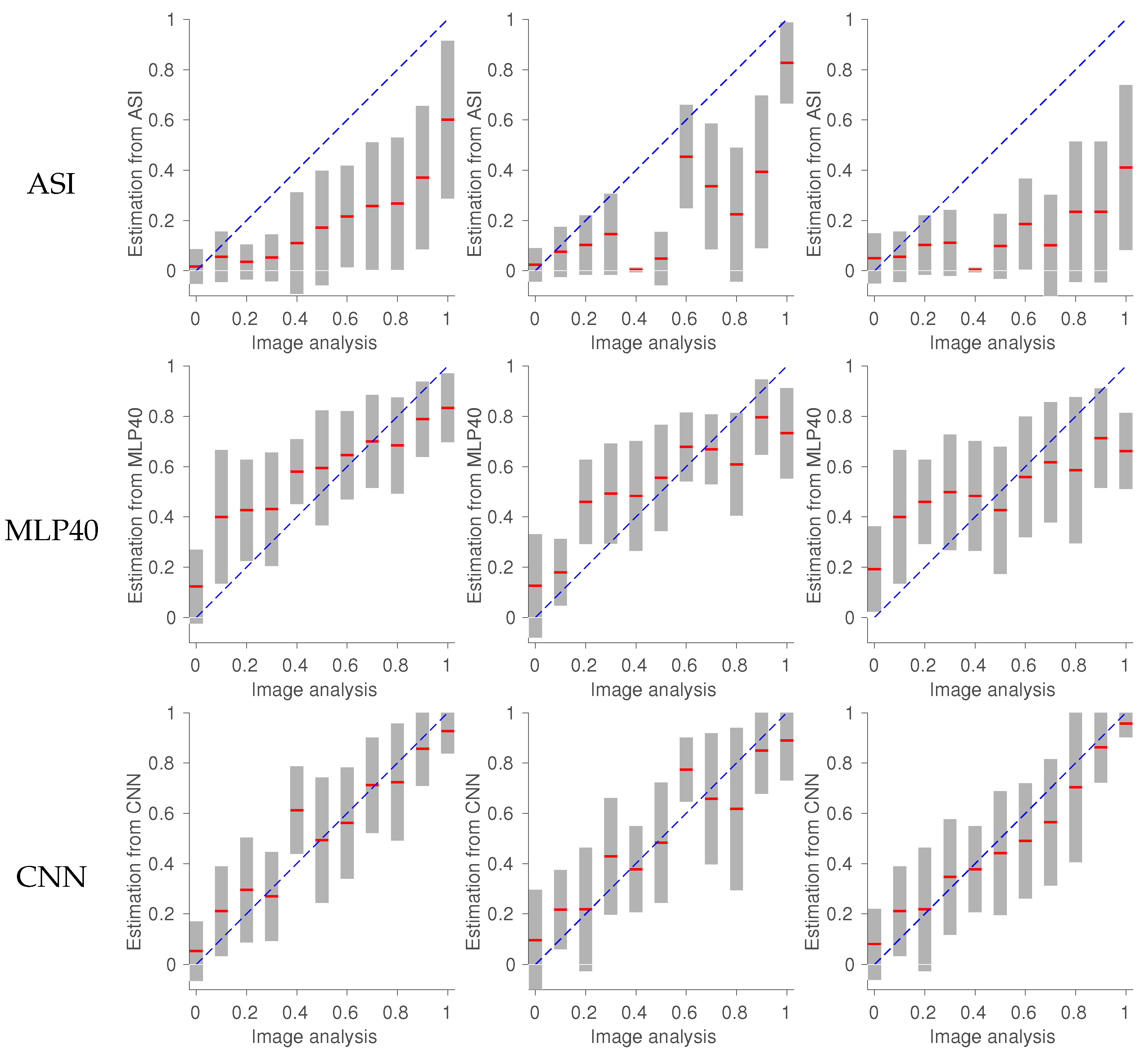
In Table 4 it can be seen that ASI underestimates ice concentration by around 24% when compared with image analyses (Table 4). Since the CNN is trained using image analysis charts, while ASI ice concentration is not, it is expected to have lower error than ASI when the error is calculated with respect to image analysis charts. Previous studies reported that the ASI ice concentration normally has errors less than 10% for intermediate and high ice concentrations [31]. The large underestimation of ice concentration observed in this study is mainly caused by the large regions of thin ice, and the magnitude of the error is consistent with that reported in other studies [16]. The underestimation of ice concentration is improved by the CNN compared to MLP40. Note that the error standard deviation ( E s t d ) for testing is at the same level as training and validation for the CNN, which indicates a low level of over-fitting for the trained CNN model. The validation errors are larger than testing errors for MLP40. This might be caused by the insufficient testing samples used, which could lead to different distributions of image surface types for validation and testing images.
Figure 2 shows the mean value of the estimated ice concentration ± one standard deviation of the ice concentration estimate errors for different ice concentration bins from the image analysis charts. Results are shown separately for training, validation and testing datasets. There is a clear trend between image analyses and ice concentration estimates generated from SAR images for all three sets in general. ASI shows underestimation for almost all ice concentration levels, with larger underestimation for higher ice concentration values. MLP40 overestimates ice concentration for water regions by about 15% for all three datasets, and underestimates ice concentration by 20% to 40% for training, testing and validation in the highest ice concentration bin. The CNN has relatively less overestimation for water regions and less underestimation for ice regions compared to MLP40. For water, CNN overestimates ice concentration on average by approximately 5% for training and 10% for testing and validation. For ice (where ice concentration is equal to 1), CNN underestimates ice concentration by less than 10% on average for all three sets. The estimation of pure water or ice generally has smaller error standard deviation than the estimate for intermediate ice concentration levels. This might be caused by the abundant water samples and ice samples in the training dataset (Figure 3), or the better quality (less errors) of ice/water samples than samples of intermediate ice concentration levels. It is reasonable to assume that the ice concentration estimates could be improved by using more training samples of intermediate ice concentration levels.

6.2. Comparison between MLP and CNN

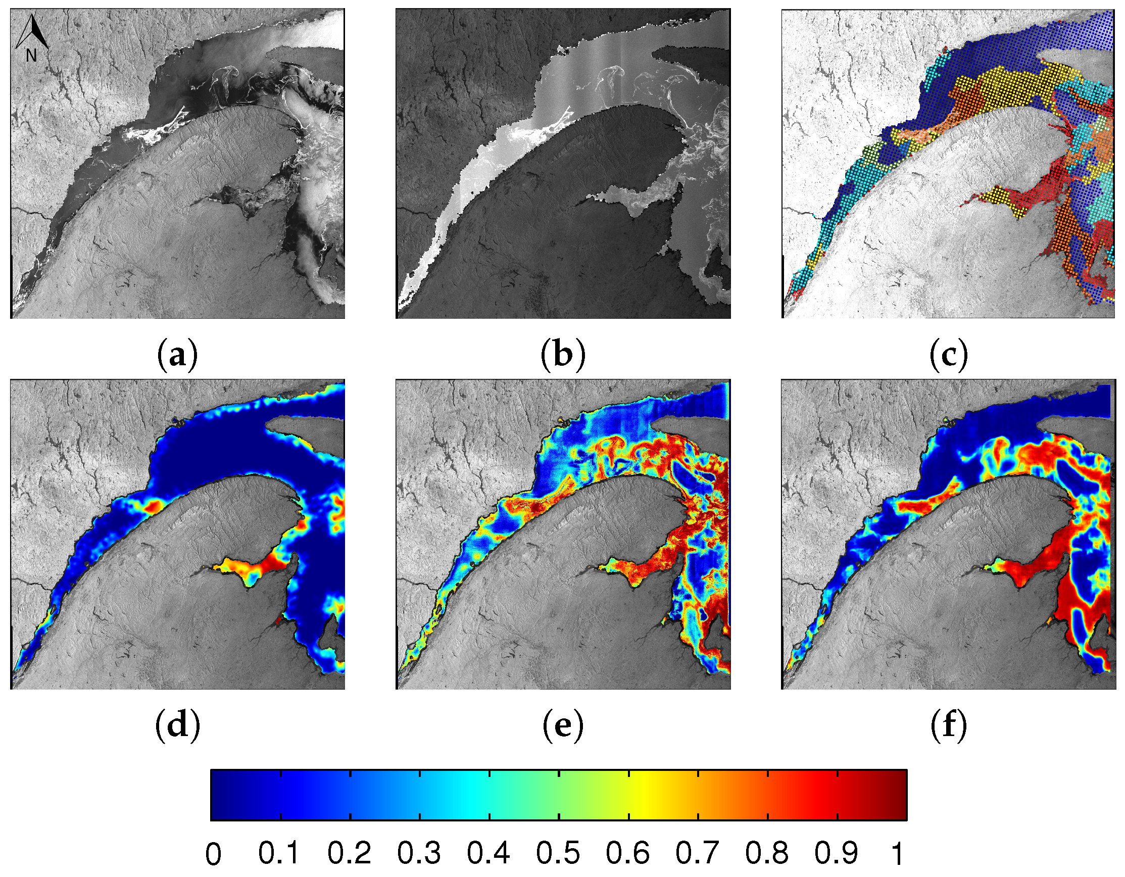
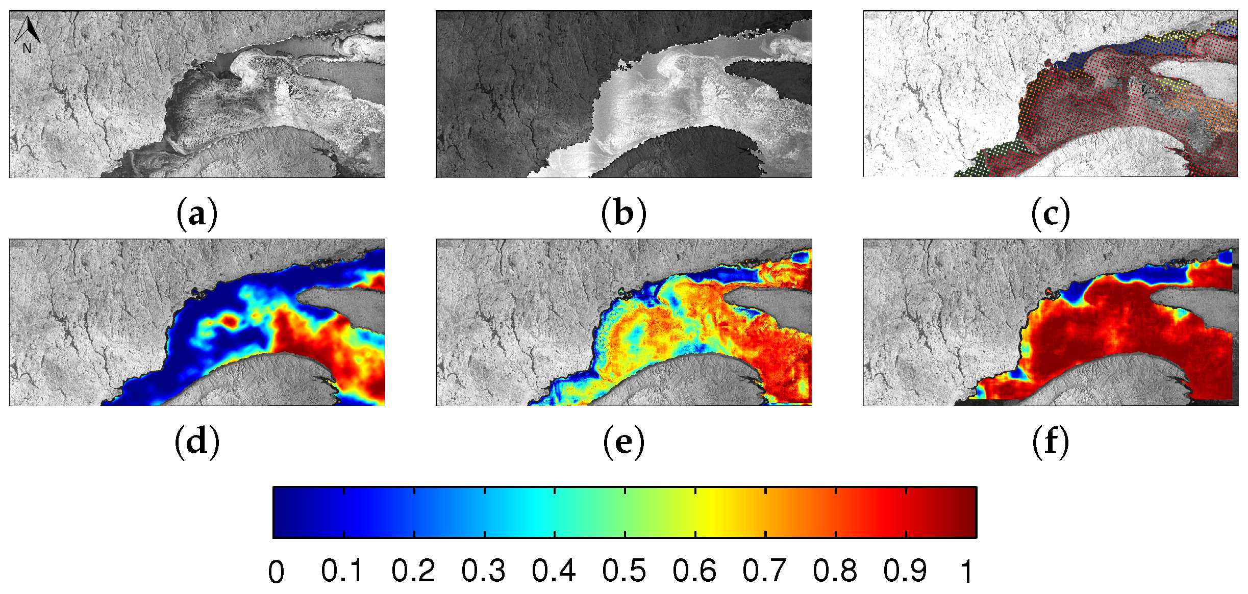
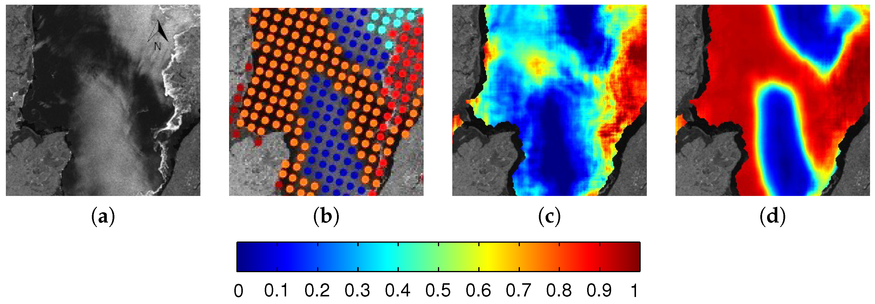
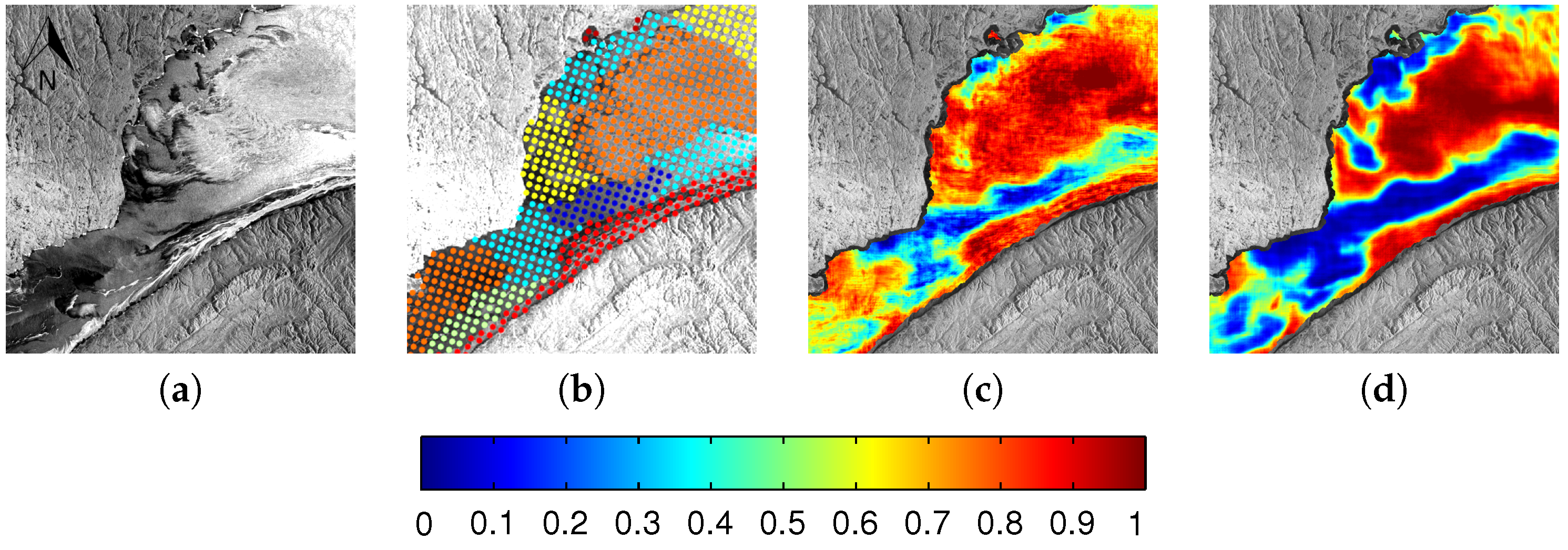
All SAR based algorithms produce ice concentration estimates with more details and sharper ice-water boundaries than the ASI data (see Figure 4 and Figure 5), which may be due to the higher resolution of SAR images, and the fact that regions of thin ice are reasonably well captured in the training data used for the SAR based methods. Figure 4e,f shows that MLP40 is more sensitive to backscatter changes in SAR images than the CNN. Therefore, MLP40 produces more details in the ice concentration estimates, as well as an ice cover that appears noisy (e.g., spurious ice can be seen over open water regions). This can sometimes introduce errors, noted in the lower left portion of Figure 6d. The ice concentration estimates by the CNN contain fewer visible errors in assignment of ice concentration than the result of MLP40, but more details than the image analysis charts, especially in low ice concentration regions and marginal ice zones (Figure 6). These differences may be caused by the difficulty to manually identify accurate boundaries of low ice concentration regions by ice analysts or the limited number of polygons they can use for each image analysis, or simply the fact that the ice charts contain an estimate of ice concentration in 10% intervals over a region (polygon) identified as homogeneous.
Strong banding in the HV channel of the RADARSAT-2 imagery may cause overestimation of ice concentration for water regions. Such an example is given in Figure 7, where MLP and CNN overestimate ice concentration for water regions with strong banding in the HV pol. The level of overestimation is reduced slightly when a larger patch size (55 vs. 45) is used for the CNN.

6.3. Evaluation of CNN Architecture and Parameters

6.3.1. Patch Size

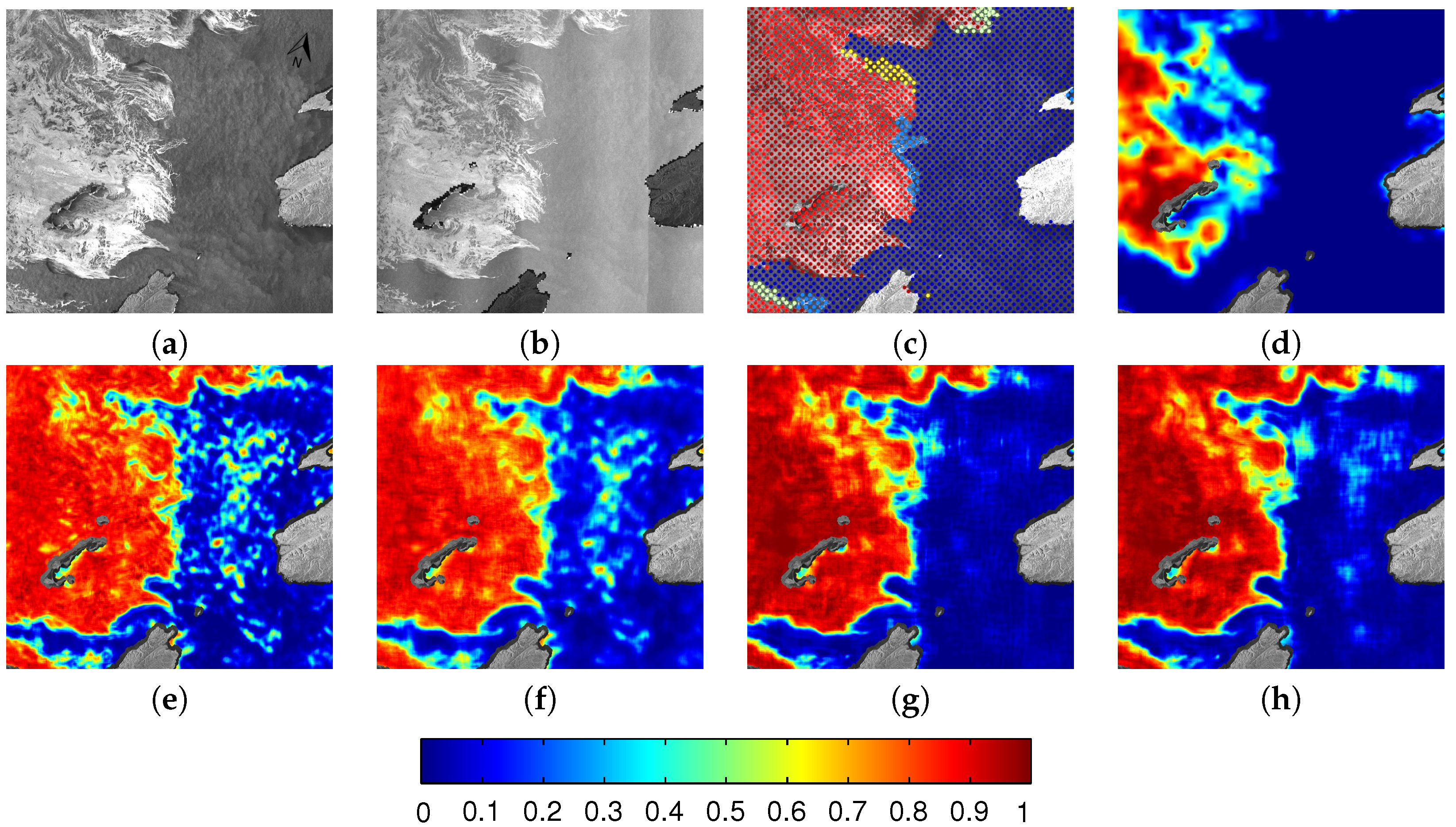
The size of the input patches, and the support of the convolutional filters, are related to the intrinsic scale and complexity of the problem. The impact of patch size was evaluated by examining the output of the CNN for patch sizes of 25, 35, 45 and 55, corresponding to 10 km (25 × 400 m), 14 km (35 × 400 m), 18 km (45 × 400 m) and 22 km (55 × 400 m). With larger patch size, the model is a better fit to the training data and the E r m s e of the training data decreases. The E r m s e for test and validation data decreases when the patch size increases from 25 to 45. However, when the patch size increased from 45 to 55, the E r m s e for the test and validation data increased slightly, which could be an indication of slight overfitting for the dataset used. Therefore, a patch size of 45 was used in this study. Note that for a different dataset, the patch size selected may be different.
The impact of patch size on the estimated ice concentration can be seen in the regions contaminated with either banding or wind roughened open water. Examples are shown in Figure 8. The smaller patch sizes (Figure 8e,f) lead to spurious ice in water regions due to wind and banding. These results suggest that the separation of water and ice requires spatial context information over a larger region. This is also seen in studies using GLCM statistics to separate ice from water, in which case the separation of the two generally improves when larger patches are considered [7]. In contrast, ice is generally well identified for all tested patch sizes. Using small patch sizes tends to slightly underestimate ice concentration, leading to ice cover that is less homogeneous, as compared to larger patch sizes. For the patch size of 25, in some cases openings (i.e., open water) can be seen in the ice cover (not shown) for polygons corresponding to 100% ice concentration in the image analysis chart.

6.3.2. Use of Incidence Angle Data

The results shown in previous sections used input image patches consisting of HH pol, HV pol and incidence angle. To investigate the impact of including incidence angle on the estimated ice concentration, CNNs are trained, validated and tested, with HH pol and HV pol only. The network structure used is the same as that for the CNN without incidence angle (Table 2). The ice concentration from the CNN is evaluated against image analysis charts, results are given in Table 5. The errors are higher in all cases when incidence angle is included. This is in part likely due to the fact that including the incidence angle information leads to greater dependency of the CNN on the HH channel. This may also be due to the fact that with a third channel of input, the model is larger (there are more weights that need to be trained), and is therefore has more potential to overfit the training data.
Due to the reduced dependency of the CNN on the HV pol, and more significant extraction of information from the HH pol with the use of incidence angle, the banding effect from HV is reduced, but the ice concentration estimates appear to be more sensitive to wind roughening. New ice is more likely to be correctly identified when incidence angle is used (Figure 9), in particular for cases when there are features visible in the HH image that appear to indicate a region of new ice.

6.3.3. Network Depth

Network depth is the number of convolutional layers in the CNN, where each layer contains a filtering, non-linear activation and pooling operation. The network depth is an important parameter that determines the level of abstraction used for classification or regression. Here, CNN models with two and three convolutional layers are trained and evaluated. In both cases, there are two fully connected layers after the convolutional layers. The error statistics against image analyses are illustrated in Table 6. Although the use of two or three convolutional layers in the networks generates similar error statistics, visually, the network with three convolutional layers produces smoother and more reasonable ice concentration estimates, as shown in Figure 10. This makes sense as deeper networks extract more abstract features so that the results are less sensitive to raw pixel values. The ice-covered regions in Figure 10a that are incorrectly identified by the network with two convolutional layers (Figure 10c) are correctly identified by the network with three convolutional layers (Figure 10d). Regions that can be visually identified as open water in Figure 11a look cleaner when three layers are used, as shown in Figure 11d. While similar results (meaning sharper features with increasing layers) are obtained when more convolutional layers are used, as adding more layers leads to increased computational complexity, the three-convolutional-layer structure is deemed adequate.

7. Discussion

In this study, a CNN has been applied to estimate sea ice concentration from dual-polarized SAR images in the Gulf of St. Lawrence. State-of-the-art ice concentration estimates with finer details than the image analysis chart are generated. Experiments using HV pol or HH pol only have also been carried out (results not shown here). Using dual-pol SAR imagery leads to improved ice concentration estimates as compared to using HH pol or HV pol only. When using HH pol only, the results are strongly affected by the incidence angle, which causes overestimation of ice concentration for water regions at low incidence angles. Using only HV pol shows banding in the estimated ice concentration. Similar results have been demonstrated in previous studies [4,52].
Sea ice concentration from image analysis charts was selected as the training data for this study. These charts contain regions (polygons) labelled by a trained analyst as having homogeneous ice conditions. When the image analysis charts were sampled, a single pixel from the image analysis (representing an area of 8 km × 5 km) was associated with a patch from the SAR image (representing an area of 18 km × 18 km). This means the SAR image patches could overlap polygon boundaries. While it may have been more appropriate to sample the image analysis charts to avoid this overlap, the accuracy of the polygon boundaries is not known. The image analyses are also subjective manual analyses, and are known to contain errors [36], as is the case with any ice concentration analysis. Even if it can be assumed the polygon boundaries are accurate, the use of spatially discrete polygons to represent the ice concentration over an image of continuous grey levels, introduces sampling errors in the ice concentration estimates. Preliminary work on the impact of errors in the training data, and alternative methods to train a CNN to estimate sea ice concentration, can be found in [53]. Learning a sparse representation of the data could improve the ice concentration estimates when training sample quality and quantity are not sufficient [54].
Testing demonstrates that the CNN is robust to the changes in image tone with incidence angle, even without explicitly including incidence angle data as an input. When the incidence angle data was included, an increased dependence on the HH pol image was observed in the ice concentration. Windspeed information could also be included as an additional input, which could help reduce the spurious ice that appears in some cases over open water when it appears to be wind-roughened. This would require accurate windspeed information at a sufficiently high spatial resolution, which is not presently available.
A linear activation function has been chosen for the last fully connected layer, which means that ice concentration values can be estimated that are greater than 1 or less than zero. For comparison between the different methods these ice concentration values were truncated to remain in the range of [0,1]. A sigmoid activation would be a more intuitive choice, as it naturally bounds the output of the CNN to 0 and 1. However, in our experiment, sigmoid activation was found to produce saturated ice concentration predictions close to 0 or 1, and large errors for intermediate ice concentration levels.

8. Conclusions

The CNN has been found to generate ice concentration estimates with improved details and accuracy as compared to ASI passive microwave ice concentration products when IA charts are used as the verification data. Our CNN ice concentration is also improved as compared to that from a method that uses an MLP to regress ice concentration from a set of engineered SAR image features. Because of the shallow network structure, MLP40 is more sensitive to the SAR image backscatter values than the CNN, which causes noisy ice concentration estimates. The small model used by MLP40 does not have the large learning capacity as the CNN. Some complex cases, such as dark new ice, are not recognized correctly. This causes systematic errors in the results, which cannot be corrected by segmentation based post-processing. Therefore, the deeper and larger CNNs used here can generate more accurate ice concentration estimates than MLP40. Note that while a multilayer version of MLP40 could be developed, maintaining full connectivity between the weights in these layers would require many weights to be learned, making such networks prone to overfitting [13]. Compared to standard fully connected neural networks with similar number of units, CNNs are able to model local spatial information more efficiently with fewer trainable parameters, which also makes them easier to train [26,55]. The success of CNNs as multi-layer networks is due to weight sharing and the local connectivity between adjacent layers [38], and methods developed to reduce overfitting [26], such as training sample augmentation and dropout, which have been implemented in the present study.
We note that there are alternative approaches to using a CNN for this problem that may be more efficient than that presented here. For example, methods that predict dense labelling as compared to a label [30,56] at a single pixel location (as has been done in the present study). Preliminary work using such an architecture for the GSL data has been presented in [53], and will be investigated further in a future study.

Acknowledgments

This study was funded through the Chinese Scholarship Council, the National Science and Engineering Research Council of Canada, ArcticNet Networks of Centres of Excellence, and the Grants and Contributions program through Environment Canada. The authors would like to thank Lynn Pogson and Alain Caya for providing the SAR imagery and image analysis charts. RADARSAT-2 Data and Products ©MacDonald, Dettwiler and Associates Ltd. 2010. All Rights Reserved. RADARSAT is an official mark of the Canadian Space Agency.

Author Contributions

Lei Wang carried out the data processing and analysis, and contributed to the research design and manuscript writing. Andrea Scott led manuscript writing, contributed to the research design and co-supervised this study. David Clausi contributed to manuscript writing and research design, and co-supervised this study.

Conflicts of Interest

The authors declare no conflict of interest.

References

  1. Carrieres, T.; Greenan, B.; Prinsenberg, S.; Peterson, I. Comparison of Canadian daily ice charts with surface observations off Newfoundland, winter 1992. Atmos. Ocean 1996, 34, 207–226. [Google Scholar] [CrossRef]
  2. Arkett, M.; Braithwaite, L.; Pestieau, P.; Carrieres, T.; Pogson, L.; Fabi, C.; Geldsetzer, T. Preparation by the Canadian Ice Service for the operational use of the RADARSAT Constellation Mission in their ice and oil spill monitoring programs. Can. J. Remote Sens. 2015, 41, 380–389. [Google Scholar] [CrossRef]
  3. Karvonen, J. Baltic sea ice concentration estimation based on C-band HH-polarized SAR data. Sel. Top. Appl. Earth Obs. Remote Sens. 2012, 5, 1874–1884. [Google Scholar] [CrossRef]
  4. Karvonen, J. Baltic sea ice concentration estimation based on C-band dual-polarized SAR data. IEEE Trans. Geosci. Remote Sens. 2014, 52, 5558–5566. [Google Scholar] [CrossRef]
  5. Clausi, D.A. Comparison and fusion of co-occurrence, Gabor, and MRF texture features for classification of SAR sea ice imagery. Atmos. Ocean 2001, 39, 183–194. [Google Scholar] [CrossRef]
  6. Deng, H.; Clausi, D.A. Unsupervised segmentation of synthetic aperture radar sea ice imagery using a novel Markov random field model. IEEE Trans. Geosci. Remote Sens. 2005, 43, 528–538. [Google Scholar] [CrossRef]
  7. Leigh, S.; Wang, Z.; Clausi, D.A. Automated ice-water classification using dual polarization SAR satellite imagery. IEEE Trans. Geosci. Remote Sens. 2014, 52, 5529–5539. [Google Scholar] [CrossRef]
  8. Zakhvatkina, N.Y.; Alexandrov, V.Y.; Johannessen, O.M.; Sandven, S.; Frolov, I.Y. Classification of Sea Ice Types in ENVISAT Synthetic Aperture Radar Images. IEEE Trans. Geosci. Remote Sens. 2013, 51, 2587–2600. [Google Scholar] [CrossRef]
  9. Liu, J.; Scott, K.; Gawish, A.; Fieguth, P. Automatic detection of the ice edge in SAR imagery using curvelet transform and active contour. Remote Sens. 2016, 8. [Google Scholar] [CrossRef]
  10. Pogson, L.; Geldsetzer, T.; Buehner, M.; Carrieres, T.; Ross, M.; Scott, K. A collection of empirically-derived characteristic values from SAR across a year of sea ice environments for use in data assimilation. Mon. Weather Rev. 2016, in press. [Google Scholar]
  11. Buehner, M.; Caya, A.; Pogson, L.; Carrieres, T.; Pestieau, P. A new Environment Canada regional ice analysis system. Atmos. Ocean 2013, 51, 18–34. [Google Scholar] [CrossRef]
  12. Drusch, M. Sea ice concentration analyses for the Baltic Sea and their impact on numerical weather prediction. J. Appl. Meteorol. Climatol. 2006, 45, 982–994. [Google Scholar] [CrossRef]
  13. LeCun, Y.; Bengio, J.; Hinton, G. Deep Learning. Nature 2015, 521, 436–444. [Google Scholar] [CrossRef] [PubMed]
  14. Wang, L.; Scott, K.A.; Xu, L.; Clausi, D.A. Sea Ice Concentration Estimation During Melt From Dual-Pol SAR Scenes Using Deep Convolutional Neural Networks: A Case Study. IEEE Trans. Geosci. Remote Sens. 2016, 54, 4524–4533. [Google Scholar] [CrossRef]
  15. Geldsetzer, T.; Yackel, J. Sea ice type and open water discrimination using dual co-polarized C-band SAR. Can. J. Remote Sens. 2009, 35, 73–84. [Google Scholar] [CrossRef]
  16. Ivanova, N.; Tonboe, R.; Pedersen, L.T. SICCI Product Validation and Algorithm Selection Report (PVASR)—Sea Ice Concentration; Technical Report; European Space Agency: Paris, France, 2013. [Google Scholar]
  17. Dumbill, E. Strata 2012: Making Data Work; O’Reilly: Santa Clara, CA, USA, 2012. [Google Scholar]
  18. Najafabadi, M.M.; Villanustre, F.; Khoshgoftaar, T.M.; Seliya, N.; Wald, R.; Muharemagic, E. Deep learning applications and challenges in big data analytics. J. Big Data 2015, 2. [Google Scholar] [CrossRef]
  19. National Research Council. Frontiers in Massive Data Analysis; The National Academies Press: Washington, DC, USA, 2013. [Google Scholar]
  20. Domingos, P. A Few Useful Things to Know About Machine Learning. Commun. ACM 2012, 55, 78–87. [Google Scholar] [CrossRef]
  21. Bengio, Y.; Courville, A.; Vincent, P. Representation learning: A review and new perspectives. IEEE Trans. Pattern Anal. Mach. Intell. 2013, 35, 1798–1828. [Google Scholar] [CrossRef] [PubMed]
  22. Hinton, G.E. Learning multiple layers of representation. Trends Cogn. Sci. 2007, 11, 428–434. [Google Scholar] [CrossRef] [PubMed]
  23. Bengio, Y. Learning deep architectures for AI. Found. Trends Mach. Learn. 2009, 2, 1–127. [Google Scholar] [CrossRef]
  24. Lee, H.; Grosse, R.; Ranganath, R.; Ng, A.Y. Convolutional deep belief networks for scalable unsupervised learning of hierarchical representations. In Proceedings of the 26th Annual International Conference on Machine Learning, Montreal, QC, Canada, 14–18 June 2009; pp. 609–616. [Google Scholar]
  25. Ciresan, D.C.; Meier, U. Flexible, high performance convolutional neural networks for image classification. In Proceedings of the Twenty-Second International Joint Conference On Artificial Intelligence, Barcelona, Spain, 16–22 July 2011; pp. 1237–1242. [Google Scholar]
  26. Krizhevsky, A.; Sutskever, I.; Hinton, G.E. ImageNet classification with deep convolutional neural networks. In Proceedings of the 25th International Conference on Neural Information Processing Systems, Lake Tahoe, NV, USA, 3–6 December 2012; pp. 1097–1105. [Google Scholar]
  27. Karpathy, A.; Toderici, G.; Shetty, S.; Leung, T.; Sukthankar, R.; Fei-Fei, L. Large-scale video classification with convolutional neural networks. In Proceedings of the 2014 IEEE Conference on Computer Vision and Pattern Recognition, Columbus, OH, USA, 23–28 June 2014; pp. 1725–1732. [Google Scholar]
  28. Mnih, V.; Hinton, G.E. Learning to detect roads in high-resolution aerial images. In Computer Vision-ECCV 2010; Springer: Berlin/Heidelberg, Germany, 2010; pp. 210–223. [Google Scholar]
  29. Chen, X.; Xiang, S.; Liu, C.L.; Pan, C.H. Vehicle Detection in Satellite Images by Hybrid Deep Convolutional Neural Networks. IEEE Geosci. Remote Sens. Lett. 2014, 11, 1797–1801. [Google Scholar] [CrossRef]
  30. Maggiori, E.; Tarabalka, Y.; Charpiat, G.; Alliez, P. Fully convolutional neural networks for remote sensing image classification. In Proceedings of the 2016 IEEE Geoscience and Remote Sensing Symposium, Beijing, China, 10–15 July 2016. [Google Scholar]
  31. Spreen, G.; Kaleschke, L.; Heygster, G. Sea ice remote sensing using AMSR-E 89-GHz channels. J. Geophys. Res. 2008, 113. [Google Scholar] [CrossRef]
  32. Agnew, T.; Howell, S. The use of operational ice charts for evaluating passive microwave ice concentration data. Atmos. Ocean 2003, 41, 317–331. [Google Scholar] [CrossRef]
  33. Karvonen, J.; Vainio, J.; Marnela, M.; Eriksson, P.; Niskanen, T. A comparison between high-resolution EO-based and ice analyst-assigned sea ice concentrations. J. Sel. Top. Appl. Earth Obs. Remote Sens. 2015, 8, 1799–1807. [Google Scholar] [CrossRef]
  34. Fequest, D. MANICE: Manual of Standard Procedures for Observing and Reporting Ice Conditions; Environment Canada: Ottawa, ON, Canada, 2002. [Google Scholar]
  35. Slade, B. RADARSAT-2 Product Description; MacDonald, Dettwiler and Associates Ltd.: Richmond, BC, Canada, 2009. [Google Scholar]
  36. Moen, A.; Doulgeris, P.; Anfinsen, S.; Renner, A.; Hughes, N.; Gerland, S.; Eltoft, T. Comparison of feature based segmentation of full polarimetric SAR satellite sea ice images with manually drawn ice charts. Cryosphere 2013, 7, 1693–1705. [Google Scholar] [CrossRef]
  37. De Andrade, A. Best Practices for Convolutional Neural Networks Applied to Object Recognition in Images; Technical Report; Department of Computer Science, University of Toronto: Toronto, ON, USA, 2014. [Google Scholar]
  38. LeCun, Y.; Bottou, L.; Bengio, Y.; Haffner, P. Gradient-based learning applied to document recognition. Proc. IEEE 1998, 86, 2278–2324. [Google Scholar] [CrossRef]
  39. LeCun, Y.; Huang, F.J.; Bottou, L. Learning methods for generic object recognition with invariance to pose and lighting. In Proceedings of the 2004 IEEE Computer Society Conference on Computer Vision and Pattern Recognition, Washington, DC, USA, 27 June–2 July 2004. [Google Scholar]
  40. LeCun, Y.; Kavukcuoglu, K.; Farabet, C. Convolutional networks and applications in vision. Proceedings of 2010 IEEE International Symposium on Circuits and Systems (ISCAS), Paris, France, 30 May–2 June 2010; pp. 253–256. [Google Scholar]
  41. Chen, L.C.; Papandreou, G.; Kokkinos, I.; Murphy, K.; Yuille, A.L. Semantic image segmentation with deep convolutional nets and fully connected CRFs. arXiv, 2016; arXiv:1412.7062. [Google Scholar]
  42. Hastie, T.; Tibshirani, R.; Friedman, J. The Elements of Statistical Learning; Springer: Berlin/Heidelberg, Germany, 2009; Volume 2. [Google Scholar]
  43. Bishop, C.M. Pattern Recognition and Machine Learning; Springer: Berlin/Heidelberg, Germany, 2006. [Google Scholar]
  44. Nair, V.; Hinton, G.E. Rectified linear units improve restricted Boltzmann machines. In Proceedings of the 27th International Conference on Machine Learning (ICML-10), Haifa, Israel, 21–24 June 2010; pp. 807–814. [Google Scholar]
  45. Scherer, D.; Müller, A.; Behnke, S. Evaluation of pooling operations in convolutional architectures for object recognition. In Artificial Neural Networks–ICANN 2010; Springer: Berlin/Heidelberg, Germany, 2010; pp. 92–101. [Google Scholar]
  46. LeCun, Y.; Bottou, L.; Orr, G.; Müller, K. Efficient backprop. In Neural Networks: Tricks of the Trade; Springer: Berlin/Heidelberg, Germany, 2012. [Google Scholar]
  47. Prechelt, L. Early stopping-but when? In Neural Networks: Tricks of the Trade; Springer: Berlin/Heidelberg, Germany, 2012; pp. 53–67. [Google Scholar]
  48. Chatfield, K.; Simonyan, K.; Vedaldi, A.; Zisserman, A. Return of the Devil in the Details: Delving Deep into Convolutional Nets. arXiv, 2014; arXiv:1405.3531. [Google Scholar]
  49. Hinton, G.E.; Srivastava, N.; Krizhevsky, A.; Sutskever, I.; Salakhutdinov, R.R. Improving neural networks by preventing co-adaptation of feature detectors. arXiv, 2012; arXiv:1207.0580. [Google Scholar]
  50. Jia, Y.; Shelhamer, E.; Donahue, J.; Karayev, S.; Long, J.; Girshick, R.; Guadarrama, S.; Darrell, T. Caffe: Convolutional architecture for fast feature embedding. In Proceedings of the ACM International Conference on Multimedia, Orlando, FL, USA, 3–7 November 2014; pp. 675–678. [Google Scholar]
  51. Watkins, J.C. Probability Theory. In Course Note for Probability Theory; University of Arizona: Tucson, AZ, USA, 2006. [Google Scholar]
  52. Wang, L.; Scott, K.; Clausi, D. Automatic feature learning of SAR images for sea ice concentration estimation using feed-forward neural networks. In Proceedings of the 2014 IEEE Geoscience and Remote Sensing Symposium, Quebec City, QC, Canada, 13–18 July 2014; pp. 3969–3971. [Google Scholar]
  53. Wang, L. Learning to Estimate Sea Ice Concentration from SAR Imagery. Ph.D. Thesis, University of Waterloo, Waterloo, ON, Canada, 2016. [Google Scholar]
  54. Wang, Q.; Lin, J.; Yuan, Y. Salient band selection for hyperspectral image classification via manifold ranking. IEEE J. Neural Netw. Learn. Syst. 2016, 27, 1279–1289. [Google Scholar] [CrossRef] [PubMed]
  55. LeCun, Y. Generalization and network design strategies. In Connections in Perspective; Elsevier: Amsterdam, The Netherlands, 1989; pp. 143–155. [Google Scholar]
  56. Maggiori, E.; Tarabalka, Y.; Chariot, G.; Alliez, P. High-resolution semantic labeling with convolutional neural networks. arXiv, 2016; arXiv:1611.01962v1. [Google Scholar]
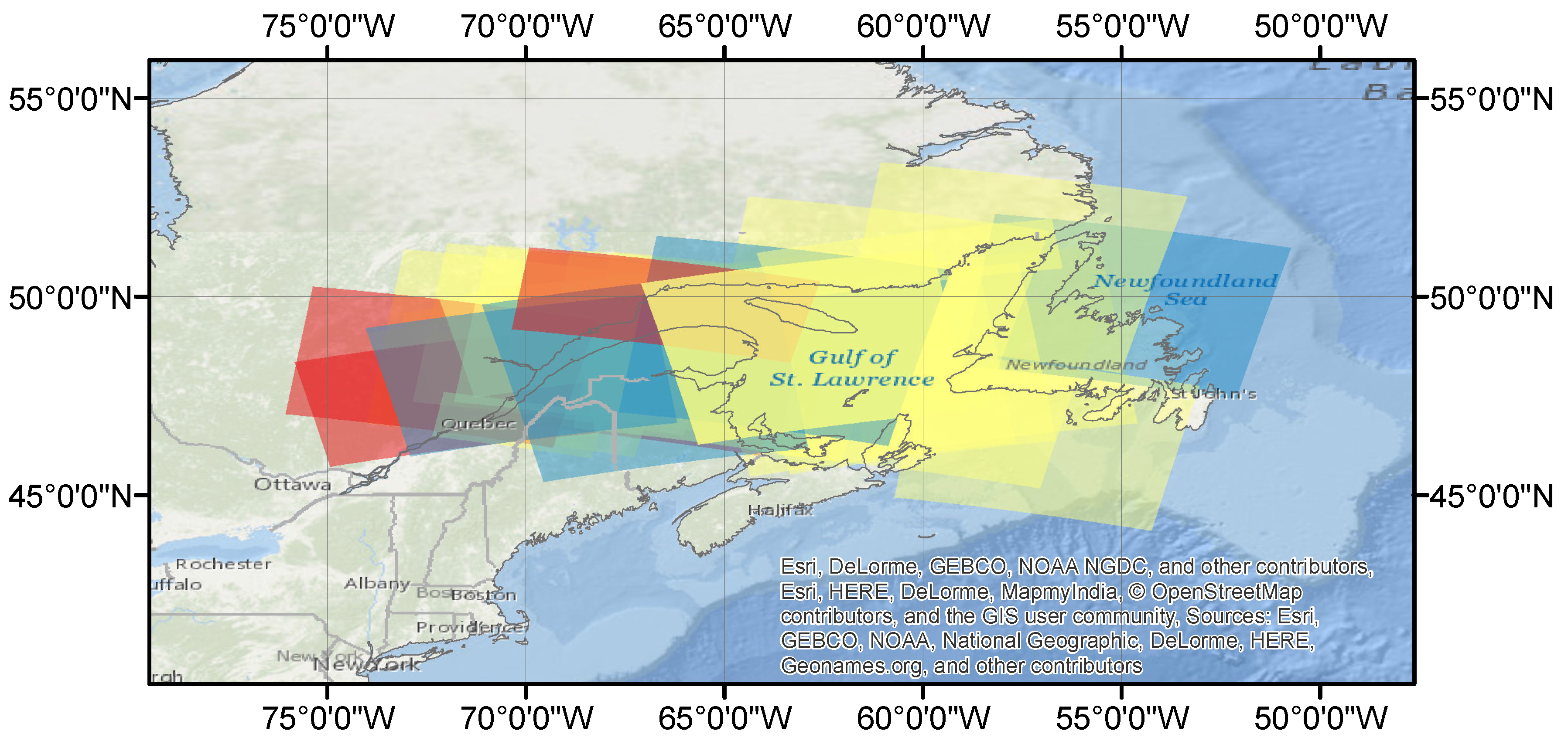
Figure 1. Study area and the dataset for the Gulf of Saint Lawrence. There are 25 scenes of dual-pol SAR images acquired between 16 January 2014 and 10 February 2014 in this area. The coverage for each scene is marked in a translucent polygon with different colors. Yellow scenes are used for training, red are used for validation and blue for testing.
Remotesensing 09 00408 g001
Figure 2. Errors at different ice concentration levels for ASI (1st row), MLP40 (2nd row), and CNN (3rd row) for training (1st column), validation (2nd column) and testing (3rd column) sets. The red lines represent the mean ice concentration, and half length of a bar represents the error standard deviation.
Remotesensing 09 00408 g002
Figure 3. Histogram of the percentage of samples from each 10% interval of the image analyses for training, validation and testing dataset of the Gulf of Saint Lawrence. The training samples are strongly biased since the majority of the training samples are either water or ice. (a) Training; (b) Validation; (c) Testing.
Remotesensing 09 00408 g003
Figure 4. Ice concentration estimated by CNN compared to that from other methods. The HH and HV images are shown in panels (a) and (b) repectively. Panel (c) is the image analysis, (df) are the ice concentration from ASI, MLP40 and CNN, repectively. Scene shown is 20140117_103914, which is used for testing. Scene centered at 47.99 N, 66.85 W with extent of 500 km by 500 km.
Remotesensing 09 00408 g004
Figure 5. Ice concentration estimated by CNN compared to that from other methods. The HH and HV images are shown in panels (a) and (b) respectively. Panel (c) is the image analysis. Panels (df) are ice concentration from ASI, MLP40 and CNN respectively. Scene shown is 20140210_103911, which is used for testing. Scene centered at 49.90 N, 66.42 W with extent of 500 km by 230 km.
Remotesensing 09 00408 g005
Figure 6. An example shows the details for a region with new ice and water. The ASI result is mainly water for this region. It can be seen MLP40 (d) produces noisy ice concentration estimates with new ice in the bottom left identified as water with some ice of low ice concentration. The CNN (e) is able to correctly identify new ice and water with higher accuracy. Subscene of dimension 60 km × 60 km from 20140117_103914 centered at 47.60 N, 64.13 W. The HH image, HV image and image analysis are shown in panels (ac) respectively.
Remotesensing 09 00408 g006
Figure 7. Example of water misidentified as ice for both MLP40 and CNN due to the banding effect in HV pol. Water in the right part of HV pol (a) is obviously brighter than water in the left. Water regions are estimated incorrectly for MLP40 (c), and CNN with patch size 45 (d). Results from the CNN are improved when a patch size of 55 is used, as shown in panel (e), although the features are also less sharp. Subscene centered at 49.72 N, 59.11 W of dimension 200 km × 200 km from 20140121_214420. Image analysis is shown in panel (b).
Remotesensing 09 00408 g007
Figure 8. Visual comparison of different patch sizes, (e) 25 × 25 pixels, (f) 35 × 35 pixels, (g) 45 × 45 pixels, (h) 55 × 55 pixels. Estimate of ice concentration is improved when patch size increases. Patch size 45, corresponding to ground distance of 18 km, has cleaner water estimates than the others. Subscene of dimension 270 km × 270 km from 20140124_215646 centered at 47.86 N, 60.94 W. Panels (ad) are the HH image, HV image, image analysis chart and ASI ice concentration respectively.
Remotesensing 09 00408 g008
Figure 9. New ice can be seen in the HH image as the dark regions along the coast (a). This ice is correctly identified when incidence angle data are used (c), as compared to when the incidence angle data is not used (d). Subscene of dimension 120 km × 52 km from 20140206_221744 centered at 47.12 N, 64.72 W. Image analysis is shown in panel (b).
Remotesensing 09 00408 g009
Figure 10. The network with three convolutional layers (d), improves the estimation for new ice compared to network with two convolutional layers (c). Panel (a) is the HH image, and (b) is the image analysis chart. Subscene of dimension 8 km × 8 km centered at 47.06 N and 64.46 W from 20140117_103914.
Remotesensing 09 00408 g010
Figure 11. Comparison of results produced by networks with two-convolutional-layer (c) and three-convolutional-layer structures (d) for a sample location centered at 49.57 N, 66.59 W with size 200 km × 200 km in scene 20140127_104734 in Gulf of Saint Lawrence. Estimate by the two-convolutional-layer network is noisier. The three-convolutional-layer network produces smoother and more reasonable results. Panel (a) is the HH image and (b) is the image analysis chart for the subregion.
Remotesensing 09 00408 g011
Table 1. Details of the Gulf of Saint Lawrence dataset. Each image analysis point covers an area of approximately 5 km × 8 km.
SetScene IDDate AcquiredNumber of Image Analysis Points
Training20140131_10305331 January 20148231
20140127_22102727 January 20141319
20140203_1043233 February 20143019
20140116_22304216 January 2014530
20140208_0957588 February 201413,872
20140210_22011110 February 20148358
20140207_2149387 February 2014612
20140125_10050025 January 20145200
20140131_21524031 January 201411,111
20140124_10350124 January 20146900
20140120_10514920 January 2014829
20140118_10100218 January 20147492
20140128_10175128 January 201412,791
20140130_22223430 January 20141407
20140123_22262723 January 2014950
20140127_10473427 January 20143427
20140124_21564624 January 201410,964
20140121_21442021 January 201415,897
Validation20140122_09524722 January 20145014
20140206_2217446 February 20143395
20140209_2230309 February 2014545
20140207_1026317 February 20149228
Testing20140210_10391110 February 20142918
20140130_11002930 January 2014425
20140126_22385026 January 2014165
20140117_10391417 January 20142922
Table 2. Structure and configuration of the CNN model used in the present study. Each row for a given layer corresponds to: the layer dimension (top row), the layer configuration (middle row) and the dimension the output (bottom row). For example for the layer Conv1 there are 64 filters of dimension 3 × 5 × 5 that are applied to an input patch of size 3 × 45 × 45 with a stride of 1 and using a pad 2, to produce an output of dimension 64 × 45 × 45 .
Layer
Data3 × 45 × 45
Conv164 × 3 × 5 × 5
stride 1, pad 2, ReLU
64 × 45 × 45
Pool12 × 2
stride 2, pad 1, Max
64 × 23 × 23
Conv2128 × 64 × 5 × 5
stride1, pad 2, ReLU
128 × 23 × 23
Pool2128 × 23 × 23
stride 2, pad 1, Max
128 × 12 × 12
Conv3128 × 128 × 5 × 5
stride 1 , pad 2 , ReLU
128 × 12 × 12
FC41024 × 128 × 5 × 5
ReLU
1024 × 1
Dropout1024 × 1 × 1
Drop rate: 0.5
1024 × 1
FC51 × 1024
Linear
1
Table 3. Image features used for method MLP40.
#PolFeature
1HVGLCM mean 25 by 25 step 5
2HHGLCM correlation 51 by 51 step 5
3HHGLCM mean 25 by 25 step 1
4HHGLCM dissimilarity 51 by 51 step 20
5HHGLCM second moment 101 by 101 step 5
6HHIntensity
7HVAverage 25 by 25 window
8HHAverage 5 by 5 window
9HHGLCM dissimilarity 51 by 51 step 5
10HHGLCM mean 101 by 101 step 20
11HVIntensity
12HH, HVHV/HH
13HH, HV(HH-HV)/HH
14HHIntensity autocorrelation
15 Incidence angle
Table 4. Average error statistics across different methods for Gulf of Saint Lawrence dataset.
MethodSet E sgn E L 1 E std E rmse
ASITraining−0.24230.26050.32070.4020
Validation−0.34160.37680.36930.5031
Testing−0.27170.28770.30970.4121
MLP40Training0.00020.14600.20500.2049
Validation−0.04100.23810.29860.3015
Testing−0.08190.17270.23250.2466
CNNTraining−0.00390.08450.15060.1507
Validation−0.01230.12530.20560.2059
Testing−0.02740.12950.21970.2214
Table 5. The average error statistics for networks trained with or without incidence angle data using CNN on the Gulf of Saint Lawrence data.
Set E sgn E L 1 E std E rmse
with incidence angleTraining−0.00390.08450.15060.1507
Validation−0.01230.12530.20560.2059
Testing−0.02740.12950.21970.2214
without incidence angleTraining0.00520.08170.14340.1435
Validation0.00350.11830.18370.1836
Testing−0.01190.12200.20310.2035
Table 6. Average error statistics for networks with two convolutional layers and three convolutional layers on the Gulf of Saint Lawrence dataset.
Two Convolutional LayersThree Convolutional Layers
Set E sgn E L 1 E std E rmse E sgn E L 1 E std E rmse
Training−0.00550.08740.12660.1269−0.00390.08450.15060.1507
Validation−0.00280.12290.19330.1934−0.01230.12530.20560.2059
Testing0.00540.15560.23000.2302−0.02740.12950.21970.2214