1. Introduction
Remote sensing image change detection is the process of identifying land cover changes by using remotely-sensed images of the same geographical area at different times [
1]. It is of high practical value in a large number of applications in diverse disciplines, such as crop growth monitoring [
2], urban sprawl detection [
3,
4], hazard assessment [
5], and snow cover monitoring [
6]. Therefore, change detection has become an attractive research topic in remote sensing communities recent years.
With the development of Earth observation programs, more and more multi-temporal synthetic aperture radar (SAR) images are available [
7]. Owning to the fact that SAR images can be obtained independently of atmospheric and sunlight conditions, SAR images are more suitable than optical or hyperspectral images to be employed in change detection. Hence, in recent decades, SAR images have been successfully applied in environmental monitoring, urban studies, and forest monitoring. However, change detection based on SAR images encounters more difficulties than that based on optical or hyperspectral images due to the presence of speckle noise [
8,
9].
In spite of the difficulties brought about by speckle noise, tremendous progress has been made in recent years, and many SAR image change detection techniques have shown impressive performance. These techniques can be categorized into two main research streams: supervised approaches and unsupervised approaches [
10]. Supervised approaches need to utilize reliable training samples to train a classifier, which will be used to classify each pixel into a changed class or an unchanged class. The samples are selected based on prior knowledge or manual labeling. On the other hand, unsupervised approaches make direct comparisons between multi-temporal images to identify the changes. Due to the fact that reliable samples are not always available, unsupervised approaches are more preferable to supervised ones. Unsupervised approaches are widely used in remote sensing communities in practice. Therefore, this paper focuses on unsupervised SAR image change detection.
Existing unsupervised SAR image change detection techniques are mainly based on difference image (DI) analysis. Generally, these techniques are often comprised of two steps [
8]: (1) DI generation by using various kinds of operators, and (2) classification of the DI into changed and unchanged classes. Since these techniques are based on DI analysis, the quality of DI is very important and affects the final change detection results. The common technique used to generate a DI is the log-ratio operator [
11,
12], since the log-ratio operator is widely acknowledged to be robust to calibration and radiometric errors.
In the DI classification step, the thresholding method and clustering method are generally used. The thresholding method is the most intuitive way to analyze the DI. Bruzzone et al. [
13] assumed that the conditional density functions of the changed and unchanged classes can be modeled by Gaussian distributions. The Expectation-Maximization (EM) iterative algorithm is used to find the optimal threshold. Later, a similar framework was proposed in [
14] by using the Kittler-Illingworth (K&I) threshold selection criterion. Celik [
15] proposed an automatic threshold technique based on Bayes theory in the wavelet domain instead of the spatial domain. These thresholding methods have achieved good performance when changed and unchanged classes have distinct modes in the histogram of DI, respectively. However, they often encounter difficulties when changed and unchanged classes are strongly overlapped or their statistical distribution cannot be modeled accurately [
16]. Therefore, clustering methods are proposed to take local region information into account. In [
17], a reformulated fuzzy local information c-means cluster algorithm (RFLICM) is proposed to classify the DI based on local information. The algorithm does not need to estimate the distribution of changed and unchanged classes, and it is robust to speckle noise due to the use of local information. Celik [
18] proposed an efficient method for change detection by using PCA and k-means clustering. In this method, the DI is divided into overlapping image blocks. A feature vector space is created by projecting the block around each pixel into eigenvector space, and then the k-means clustering algorithm is employed to cluster the feature vector space into changed and unchanged classes. Li et al. [
19] proposed a novel change detection method based on two-level clustering. Two-level clustering is designed in Gabor feature space by successively combining the first-level fuzzy c-means (FCM) clustering with the second-level nearest neighbor rule. In the optical image change detection community, the contextual information is an important factor in DI analysis. Lv and Zhong [
20] proposed a multi-feature probabilistic ensemble conditional random field model for DI analysis. In this method, morphological operators are used to keep the main structure of the changed regions, and spatial contextual information is considered by the pairwise potential designed in the conditional random field model.
Several recent publications have formulated unsupervised change detection problem as an incremental learning problem. To be specific, the process of change detection simulates the learning process of humans [
21]. Humans learn to understand the world by prior knowledge provided by predecessors, through which each forms his own interpretations of the world. Similarly, the change detection task can be formulated as the following steps: First, an initial change map is generated by thresholding or clustering algorithms. Second, samples are selected from the change map and fed into a learning system as prior knowledge. Finally, the system gives its own interpretations of multi-temporal SAR images and generates a final change map. Liu et al. [
21] established a deep neural network using stacked Restricted Boltzmann Machines (RBM) to analyze the DI. In [
22], a joint classifier based on FCM was designed to select reliable samples, and then a two-layer RBM network was established for image change detection. Liu et al. [
23] proposed a deep network comprised of one convolutional layer and several coupling layers. The network performs well in heterogeneous optical and SAR image change detection. In the optical image change detection community, deep architectures have been successfully exploited for feature representations in change detections. Zhang et al. [
24] proposed a framework for multi-spatial resolution image change detection, which incorporates deep architecture-based feature learning. In the framework, stacked denoising autoencoders are integrated for learning high-level features from raw image data. Zhong et al. [
25] proposed a method based on pulse-coupled neural networks (PCNN) and normalized moment of inertia (NMI) feature analysis. The method can provide better performance for high spatial resolution optical images. In deep learning, the hierarchical structure can learn different features at different layers, and these features can represent the change information between multi-temporal images. Therefore, the available methods that depend on deep learning can obtain excellent results. In a recent technical tutorial [
26], Zhang et al. systematically reviewed state-of-the-art deep learning techniques in remote sensing data analysis. They pointed out that deep learning can automatically obtain high-level semantic features from raw data in a hierarchical manner, while traditional shallow models can hardly uncover high-level data representations.
Deep learning methods may perform poorly when the number of training samples is relative small. Generally, millions of training samples are necessary to obtain a model with powerful feature representation capability. However, this is nearly impossible for the task of SAR image change detection [
27,
28]. Though deep learning-based methods are promising, the problem of limited samples must be solved. Zou and Shi [
29] proposed SVD networks, which are designed based on the recent popular convolutional neural networks to solve the problem of ship detection in optical images. These networks can efficiently learn features from remote sensing images. Inspired by Zou’s method [
29], in this paper, we put forward a simple change detection scheme for SAR images based on deep semi-nonnegative matrix factorization (Deep Semi-NMF) and SVD networks. Inspired by the aforementioned methods, this paper formulates the change detection problem as an incremental learning problem. Deep Semi-NMF is first utilized for feature extraction, and the hierarchical FCM clustering algorithm is used to select sample pixels that have high probabilities of being changed or unchanged. Then, image patches centered at these sample pixels are generated, and these patches are used to train a model by SVD networks. Finally, pixels in the multi-temporal images are classified by the model. The SVD network classification result and the pre-classification result are combined to form the final change detection result.
The main contribution of this paper can be summarized as the following two aspects. First, we put forward a pre-classification scheme based on Deep Semi-NMF and hierarchical FCM to obtain labeled samples of high accuracy. Second, we propose a classification model based on SVD networks for change detection. SVD networks can learn nonlinear relations from multi-temporal SAR images, and are able to suppress the noisy unchanged regions. The proposed change detection method makes no rigorous assumption and is unsupervised. Therefore, it can be easily adapted for data across different SAR sensors.
This paper is organized into four sections.
Section 2 elaborates on the framework of the proposed change detection method.
Section 3 analyzes the accuracy of change detection on several real SAR datasets.
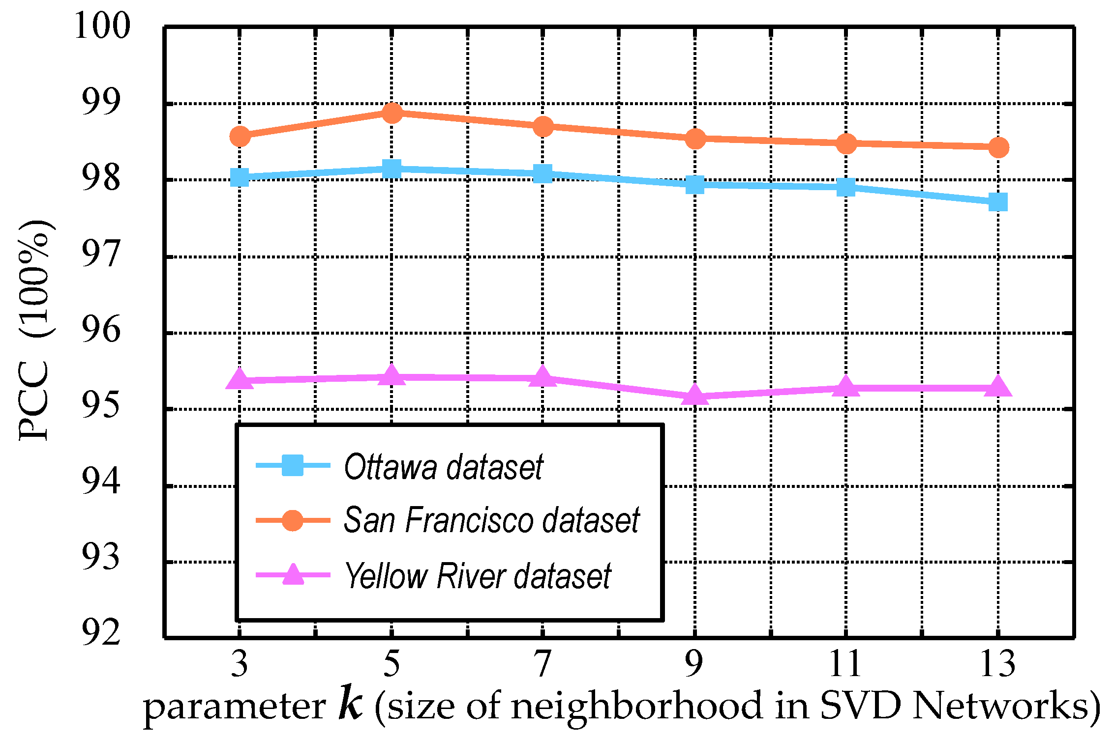
Section 4 first analyzes the influence of related parameters on the performance of change detection, and then discusses the performance of the proposed method with closely related methods. Finally,
Section 5 makes concluding remarks on the proposed method.
2. Change Detection Methodology
Let us consider two co-registered intensity SAR images and acquired over the same geographical area at two different times. Both images are of pixels. The purpose of change detection is to produce a difference image that can represent the change information between the two times in the scene. The final output of the change detection analysis is to produce a binary image associated with changed and unchanged pixels by dividing the difference image into two classes.
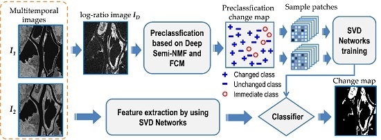
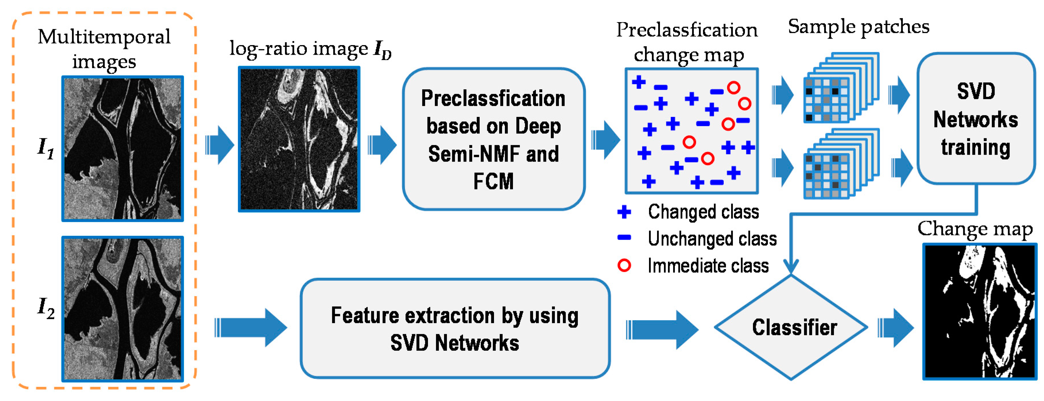
Figure 1 shows the pipeline of the proposed change detection method. The proposed method is mainly comprised of three steps:
Step 1—Pre-classification based on Deep Semi-NMF and hierarchical FCM. The log-ratio operator is first utilized to generate the log-ratio image. Then, Deep Semi-NMF is adopted for feature extraction. The hierarchical FCM algorithm is utilized for feature classification and pixels in the log-ratio image are partitioned into three groups: the changed class , the unchanged class , and the intermediate class . Pixels from and are selected as training samples for SVD networks.
Step 2—Training a classifier by SVD networks. Image patches centered at interested pixels obtained in Step 1 are generated from multi-temporal SAR images. Pixel-wise features are extracted directly from these patches. Then, SVD networks comprised of two SVD convolutional layers and one histogram feature generation layer are built. By using SVD networks, a classifier based on pixel-wise patch features is trained.
Step 3—Classification of changed and unchanged pixels by using the pretrained classifier. Pixels belonging to the intermediate class are classified into changed and unchanged class by using the classifier obtained in Step 2. Then, the classification result and the pre-classification result generated in Step 1 are combined to form the final change map.
Section 2 is organized as follows.
Section 2.1 gives the detailed description of pre-classification based on Deep Semi-NMF and hierarchical FCM clustering.
Section 2.2 introduces the process of classification by using SVD networks.
2.1. Pre-classification Based on Deep Semi-NMF and Hierarchical FCM Clustering
The first step of the proposed change detection method is pre-classification, which aims to select reliable samples for SVD networks. This subsection details the pre-classification process based on Deep Semi-NMF and hierarchical FCM.
Section 2.1.1 reviews the Deep Semi-NMF briefly.
Section 2.1.2 introduces the detailed strategy for pre-classification.
2.1.1. Deep Semi-NMF
Nonnegative Matrix Factorization (NMF) is useful to find representations of nonnegative data. It can approximate a nonnegative matrix with the product of two low-dimensional nonnegative matrices. NMF allows only additive combinations, and therefore the nonnegative constraints of NMF lead to a parts-based representation [
30]. The parts-based property makes NMF suitable for a broad range of applications, such as hyperspectral image unmixing [
31,
32], face recognition [
33], and image classification [
34]. In [
27], Zhang et al. presented an elegant solution for high dimensional remote sensing data analysis. They pointed out that matrix factorization is an important tool to extract significant features for remote sensing data analysis. Therefore, it is plausible to use matrix factorization for SAR image feature explorations.
Given an
nonnegative data matrix
and a pre-specified positive integer
, NMF aims to find two nonnegative matrices
and
, such that:
It should be noted that is a pre-specified positive integer. The value of is relatively small, so that . Thus, is considered as a new representation of the original data matrix . is considered as the mapping between the new representation and the original data matrix .
In many real world applications, the data matrix
often has mixed signs. Considering this, Ding et al. [
35] proposed the Semi-NMF, which can impose non-negativity constraints only on the second factor
, but allows mixed signs in both the data matrices
and
. The Semi-NMF has been considered to be equivalent to
k-means clustering, and it has been expected to perform better than
k-means clustering particularly when the input data is not distributed in a spherical manner.
It is considered that the mapping
contains complex hierarchical and structural hidden representations. By further factorizing the mapping
, we can automatically learn the hidden representations and obtain better higher-level feature representations of the original data matrix
. Inspired by this, Trigeorgis et al. [
36] proposed Deep Semi-NMF, which applies Semi-NMF to a multi-layer structure in order to learn hidden representations of the original data matrix. Specifically, the input data matrix is factorized into
factors as follows:
Here,
means that a matrix is allowed to have mixes signs, and
means that a matrix is comprised of strictly nonnegative components. This can be viewed as learning a hierarchical structure of features, with each layer learning a representation suitable for clustering according to the different attributes of the input data. The input data can be represented by a hierarchy of
layers as follows:
The implicit representations (
,
,
) are also restricted to be nonnegative. Therefore, each layer of this hierarchy of representations also lends itself to be a clustering interpretation. By doing this, the model can find low-dimensional representations of the input data matrix. In [
36], the Deep Semi-NMF model is able to outperform the single-layer Semi-NMF in a human face identification task. In [
37], Deep NMF is utilized in speech separation, and the experimental results show that Deep NMF outperforms the single-layer NMF in terms of the source-to-distortion ratio (SDR). This research proved that the low-dimensional representations generated by Deep Semi-NMF are better suited for clustering.
2.1.2. Strategy for Pre-classification
Traditional methods can hardly discriminate change and unchanged pixels directly. Therefore, we aim to use a deep learning-based method to improve the performance of pixel classification. The change detection task is treated as an incremental learning problem in this paper. An initial change map is generated through the pre-classification process. Pixels in the input images are classified into three groups: the changed class , the unchanged class , and the intermediate class . Pixels belonging to and have high probabilities of being changed and unchanged, respectively. These pixels are the training samples for SVD networks to generate a classifier. By using the classifier, pixels belonging to can be further classified into changed and unchanged. Then, the SVD networks classification result and the pre-classification result can be combined to form the final change map. The intermediate class can be viewed as the bridge between the pre-classification stage and the SVD networks classification stage.
In order to deal with the speckle noise in both SAR images, the well-known log-ratio operator [
1,
14,
23] is applied to generate the difference image (DI). Let
be the DI, and it can be com-puted pixel by pixel from
and
by:
The log-ratio operator is usually expressed in absolute value form. It is worth noting that the absolute value form is empirically verified to be robust to calibration errors. Based on these considerations, we adopt the log-ratio operator in the proposed change detection method.
After obtaining the difference image, the next step is to extract features by using Deep Semi-NMF. Neighborhood patches of the size
pixels around each pixel are extracted and these patches are rearranged as column vectors. Then, the column vectors for all the pixels are combined to form a
data matrix
. The process of data matrix
generation is illustrated in
Figure 2.
The factorization algorithm starts from
and
, where usually
and
are randomly initialized matrices. Here, to speed up the convergence rate of NMF, Nonnegative Double Singular Value decomposition (NNDSVD) is used. Another important issue that can affect the performance of pre-classification is the structure of Deep Semi-NMF. As empirically verified in [
36], the two-layer model is generally sufficient to achieve good performance, and a higher number of layers does not seem to lead to significant improvements. Therefore, we implement Deep Semi-NMF with a first hidden representation
with
features, and a second representation
with
features.
is the mathematical ceiling operator that maps a real number to the smallest following integer.
is a matrix with
rows and
columns. The matrix denotes the low-dimensional representation of all the pixels in the DI. Then we implement the FCM algorithm on the matrix to partition the pixels in the DI into three groups: the changed class
, the unchanged class
, and the intermediate class
. Pixels belonging to
have a high probability of being changed, and pixels belonging to
have a high probability of being unchanged. Therefore, these two kinds of pixels can be chosen as samples. We use the hierarchical FCM clustering algorithm [
38] for classification. We observed that if we directly classify pixels into three classes by FCM, the intermediate class often occupies a large part, and then we can hardly obtain enough representative samples for SVD networks training. Therefore, the FCM algorithm is organized in a cascade way to implement a coarse-to-fine procedure to guarantee efficiency. Finally, we obtain the pre-classification change map with labels
. Pixels belonging to
and
are selected as training samples.
The number of samples is a critical issue for the classification task. In our implementations, 8% of pixels from and are randomly selected as training samples. Moreover, we have empirically observed that these training samples are in general sufficient to achieve good performance and that more training samples do not necessarily lead to further improvement. In the next subsection, we will describe how to classify the pixels belonging to .
2.2. Classification by Using SVD Networks
In order to accurately identify the changed regions between multi-temporal SAR images, the analysis of the nonlinear relations from both input images is very important. In this paper, SVD networks are utilized as the classifier. The merits of SVD networks lay in the fact that features are not designed by human engineers but are learnt from the image raw data by hierarchical structures. Thus, SVD networks are able to obtain better interpretations of the nonlinear relations from the image raw data.
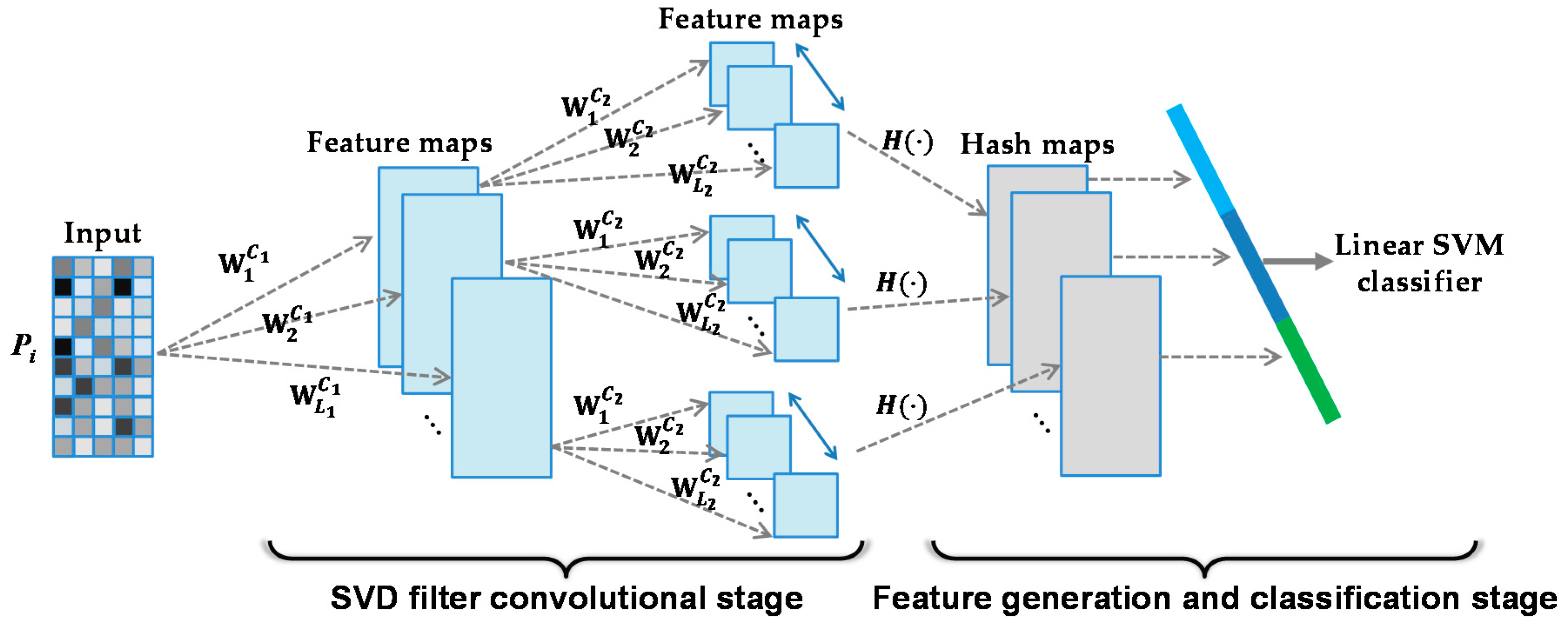
The structure of SVD networks is shown in
Figure 3. In the SVD filter convolutional stage, we use two convolutional layers. In the feature generation and classification stage, hash coding and linear SVM classifier are utilized. In the next subsections, we will give a detailed introduction of the two stages of SVD networks.
2.2.1. Stage 1: SVD Filter Convolutional Stage
In the SVD filter convolutional stage, sample image patches around sample pixels (belonging to
and
) are generated first. The sample image patches generation process is shown in
Figure 4. These patches contain local change information at the same positions. In image
, the sample patch at the central pixel
is defined as
,
. The size of
is
. At the same time, the corresponding sample patch in image
at the central pixel
is defined as
. Both patches are concatenated into a new image patch
, and the size of
is
. We randomly choose
samples to obtain the sample images
,
.
After sample image patches generation, we obtain
sample images
,
. These image patches are fed into two SVD convolutional layers. The filter banks of the first and second convolutional layers are denoted as:
where
and
represent the number of filters in the first and second convolutional layers, respectively. The
mth output map of the first convolutional layer can be denoted as:
Then, the output map of the second convolution layer can be represented as:
We use primary filters in the first convolutional layer, and then we obtain feature maps. In the second convolutional layer, each feature map is an individual input, and the output can be regarded as groups of features maps. Since we use primary filters in the second convolutional layer, we obtain feature maps in total. SVD networks are utilized as the filters to obtain the feature maps, and they are capable of exploiting the abstract semantics of the image data. Next, we give a brief review of the SVD algorithm and then introduce how SVD is used in the two convolutional layers.
SVD is a simple yet effective algorithm for extracting the dominant features by projecting the original high dimensional space into low semantic dimensional space. Compared with other feature reduction methods or feature learning methods, such as linear discriminant analysis and principal component analysis, SVD makes use of the relationships between features to establish underlying semantic means. An enriched feature space with a small number of features is established to represent the original data. Therefore, SVD can not only reduce the dimensionality, but also improve the feature classification performance. Deep learning methods may perform poorly when the number of training samples is relatively small. However, it is nearly impossible for the task of SAR image change detection to obtain tens of millions of training samples. We select SVD as the convolutional filter because it is theoretically sound, robust, and structurally compact. It is empirically verified that it performs better than principal component analysis and linear discriminant analysis.
As mentioned above, in the process of sample image patches generation, we obtain
sample images
,
. In the first convolutional layer, the pixels of each sample image are reshaped into a vector
, and all the vectors are combined into a matrix
. Then, the SVD of the data matrix
is a factorization as follows:
where
is a rectangular diagonal matrix with nonnegative real numbers on its diagonal. The diagonal entries of
are known as the singular values of
.
and
are two orthogonal matrices. The columns of
are called the left-singular vectors of
, and the columns of
are called the right-singular vectors of
. In this paper, the left-singular vectors of
with the largest
singular values are selected as the primary filter banks of the
layer.
The filter banks can be obtained by reforming back into the 2-D filters.
In the
layer, the input is
feature maps. The feature maps are reshaped into a vector
,
. All vectors are combined into a data matrix
. Therefore, the data matrix
is factorized as follows:
where
is a rectangular diagonal matrix containing singular values of
.
is an orthogonal matrix containing left-singular vectors of
.
is an orthogonal matrix containing right-singular vectors of
. Similar to the first convolutional layer, the left-singular vectors of
with the largest
singular values are selected as the primary filter banks of the
layer. The filter banks
are obtained by reforming
back into the 2-D filters.
2.2.2. Stage 2: Feature Generation and Classification Stage
Through two convolutional layers, we obtain
group outputs, and each group contains
feature maps. Then, each feature map is binarized using a Heaviside step function whose value is one for positive input and zero otherwise. Then, in each group of feature maps, around the same position we have
binary bits. For the
th group of the
binary bits, they can be encoded into a decimal number as follows:
Then, the output feature maps
are converted into
groups of integer-valued “images”
, where the value of each pixel is in the range
. Then, the histogram of
are calculated, and form a feature vector
. Finally, all the feature vectors of the same group are further concatenated together to form the final change map to form the final feature descriptor of the input image
, i.e.,
Then, the feature descriptors of all the sample images are fed into the linear SVM to train a model. By using the model, pixels belonging to are further separated into changed and unchanged classes. Finally, we combine the SVD networks classification result and the pre-classification result together to form the final change map. We have tried different numbers of layers in the SVD networks. From the experimental results, we have found that two layers for feature extraction is sufficient to achieve good performance. Therefore, in our implementations, we set the number of layers for feature extraction to two. Moreover, the SVD filter number and also affects the classification performance slightly when and are set larger than six. Inspired by Gabor filters and histogram of oriented gradients (HOG), the common settings of filters often have eight orientations, therefore, and are set as eight in our implementations.
5. Conclusions
In this paper, we proposed a novel SAR image change detection method based on Deep Semi-NMF and SVD Networks. In the proposed method, Deep Semi-NMF is used for pre-classification, and reliable samples of high accuracy can be obtained. In addition, nonlinear relations of multi-temporal SAR images can be exploited by SVD networks. We use two SVD convolutional layers to obtain reliable features, which effectively improve the classification performance. The proposed method makes no rigorous assumption and is unsupervised. Therefore, it can be easily adapted for data across different SAR sensors. The experimental results have demonstrated the effectiveness of the proposed method on three SAR image datasets.
The proposed method is a promising tool to detect changed regions for multi-temporal SAR images. However, it is still challenging to change point targets, such as aircrafts at an airport and cars in a parking lot. Therefore, in the future, we will conduct research on detecting change point targets. In addition, as more and more multisource remote sensing data covering the same area are available, it is demanding to develop change detection techniques for multisource data. Therefore, we will continue to investigate the proposed method to detect changes from multisource data. Moreover, if a series of multi-temporal SAR images are used for change detection, the spatial and temporal dynamics of a specified region can be obtained. The spatial and temporal dynamics can provide predictions of likely changes in the future. They can also provide intricate information for effective planning and management activities. In the future, we will continue our work on investigating change detection by using a series of multi-temporal SAR images.


