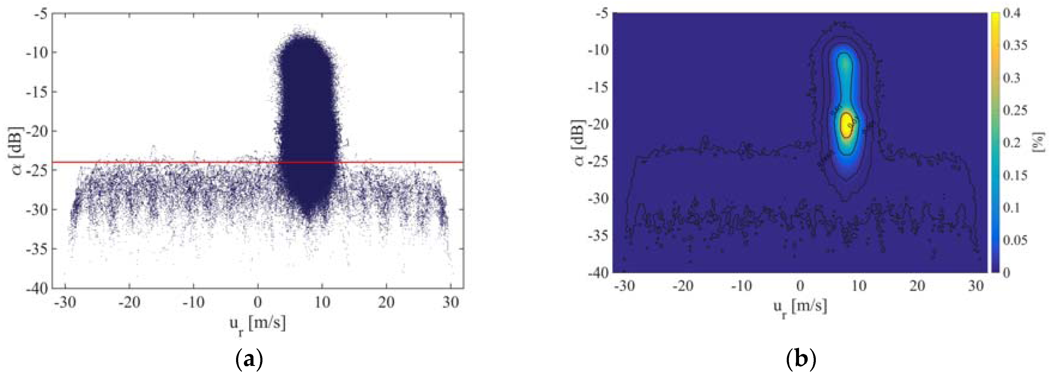
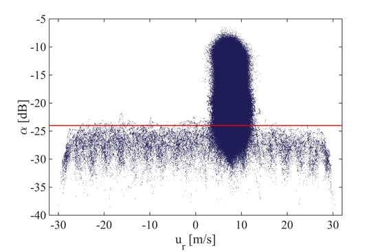
Figure 1.
Example of a staring mode LiDAR measurement in the diagram for a duration of 30 min in distances in the range of 361 m to 2911 m. (a) Blue points represent single measurements points, the red horizontal line indicates the lower CNR-threshold of −24 dB. (b) Visualisation of data density of measurement point distribution. Colours indicate different values of frequency distribution.
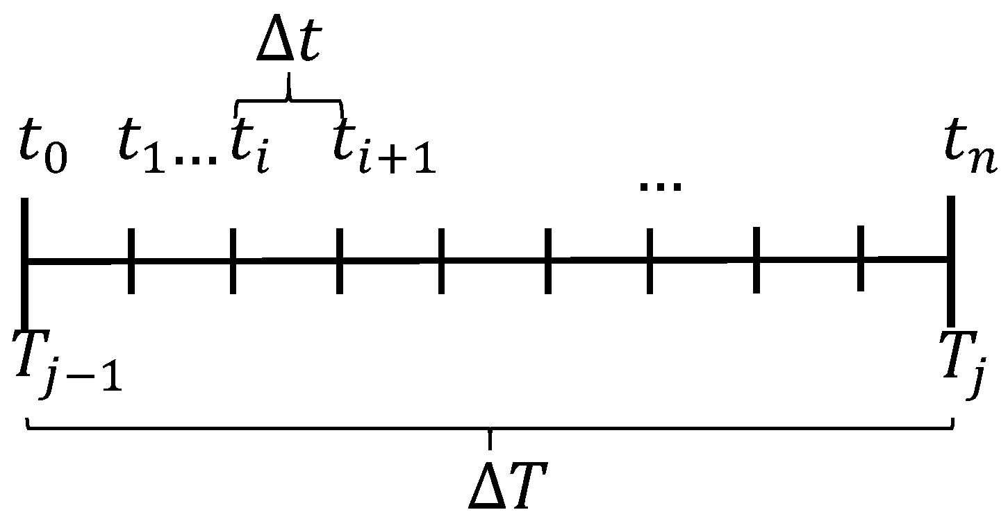
Figure 2.
Visualisation of segmentation of the overall filtering time interval in normalisation intervals .
Figure 2.
Visualisation of segmentation of the overall filtering time interval in normalisation intervals .
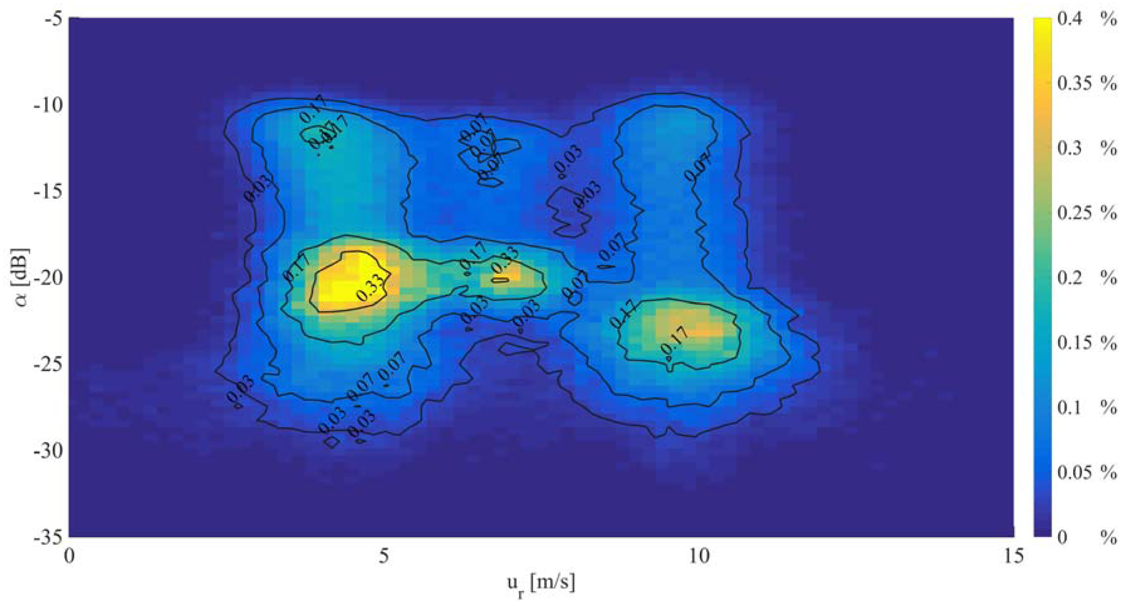
Figure 3.
Example of data-density distribution of a 30-min time interval of LiDAR staring mode measurements in the original frames of reference. Iso-lines show levels of probability of occurrence of the measurement with in a bin of 0.32 m/s width and 0.2 dB height.
Figure 3.
Example of data-density distribution of a 30-min time interval of LiDAR staring mode measurements in the original frames of reference. Iso-lines show levels of probability of occurrence of the measurement with in a bin of 0.32 m/s width and 0.2 dB height.
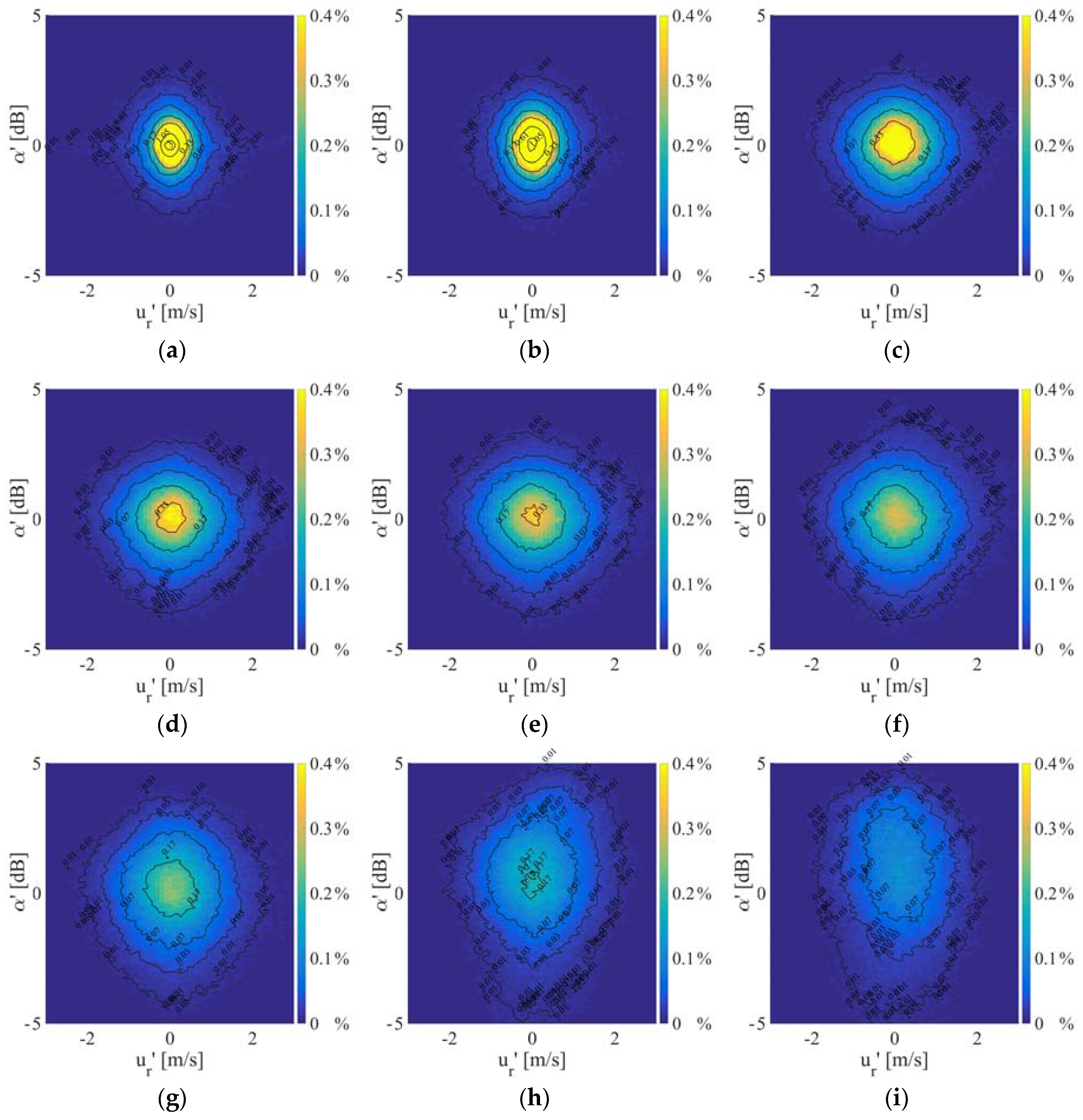
Figure 4.
Visualisation of different normalisation times of the LiDAR data distribution in the normalised frame of reference (a) (b) (c) (d) (e) (f) (g) (h) (i) .
Figure 4.
Visualisation of different normalisation times of the LiDAR data distribution in the normalised frame of reference (a) (b) (c) (d) (e) (f) (g) (h) (i) .
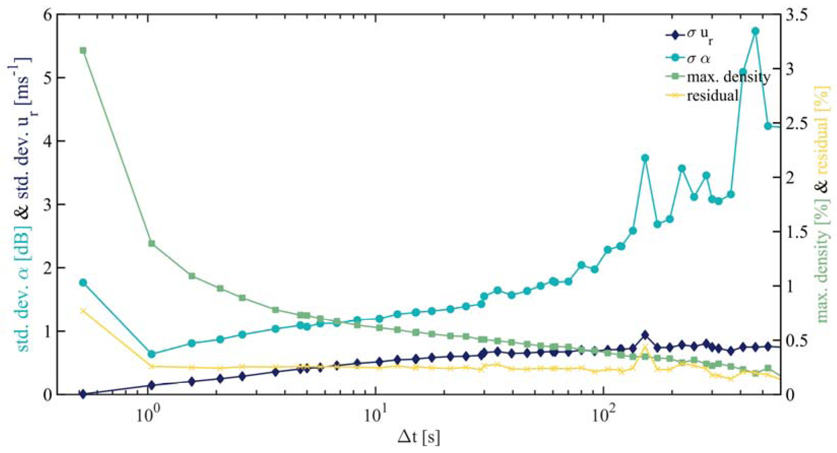
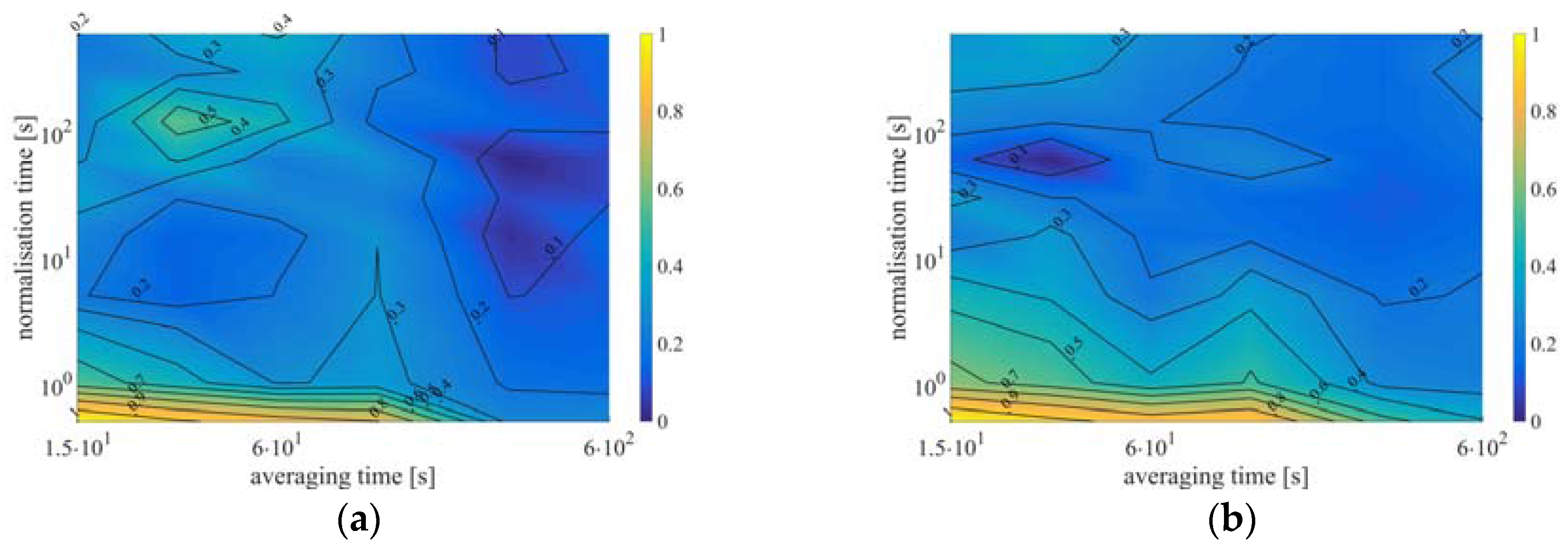
Figure 5.
Behaviour of parametrisation of fitted bi-variate Gaussian distribution of data density in relation to the different normalisation time intervals . The -axis fitted standard deviation is shown in turquoise, -axis fitted standard deviation in dark blue, the maximum probability of occurrence in green and the residual of the original and the fitted data distribution.
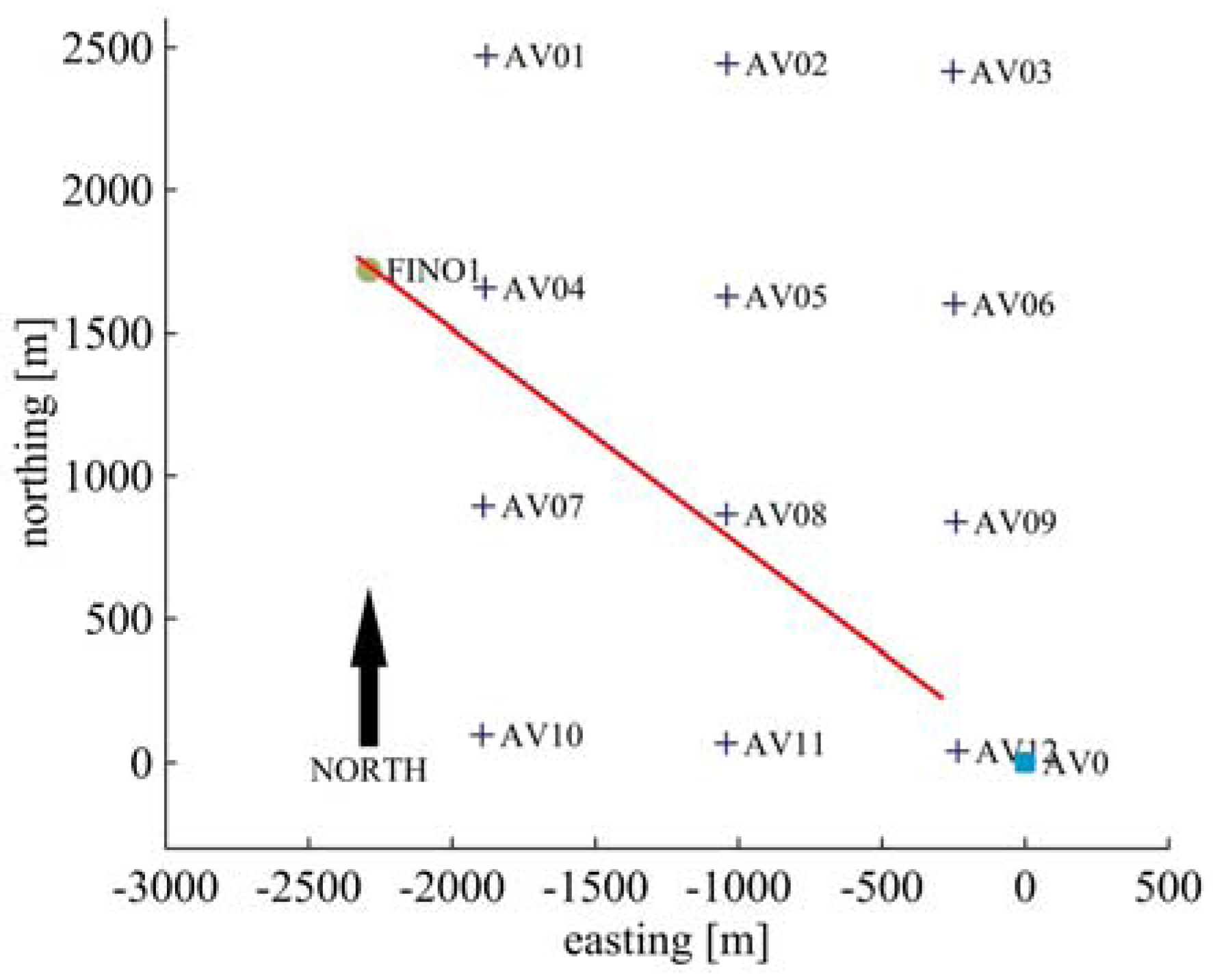
Figure 6.
Layout of the wind farm “alpha ventus” with measurement geometry of staring mode LiDAR with an azimuthal orientation of 306.47° and an elevation of 0.2° (red). Crosses represent wind turbines, the circle the platform FINO1 and the square the substation AV0. The measurement positions are indicated by the red line.
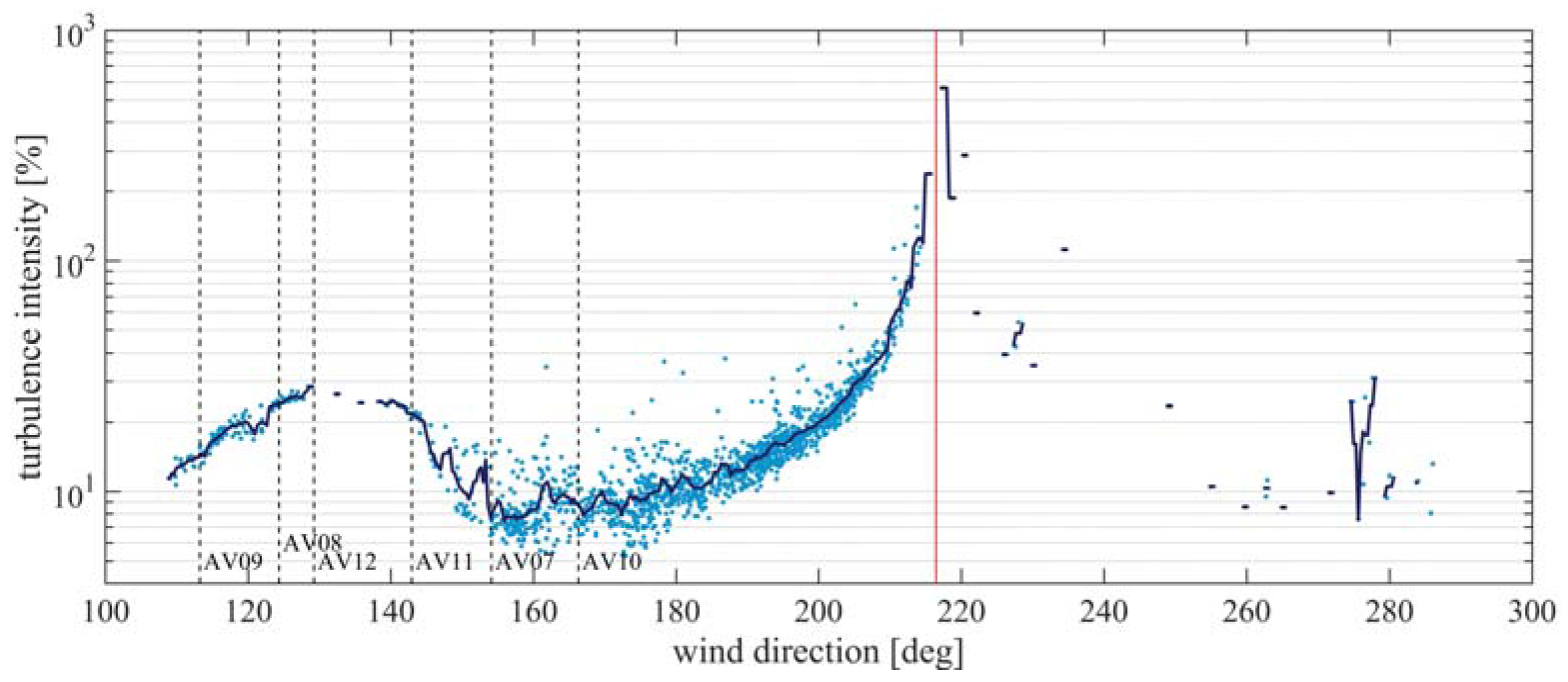
Figure 7.
Visualisation of the line-of-sight velocity turbulence intensity in dependency of the wind direction measured by the ultrasonic anemometer from 21.12.2013 15:35 h (UTC) till 19.01.2014 7:55 h (UTC). Gaps in the plot visualise unavailability of anemometer data. Individual 10 min mean values are shown in light blue whereas the binned averaged is marked in dark blue. Black vertical dashed lines indicate the wind direction of possible wake shading of the anemometer on FINO1 based on geometrical correlations. The red line shows the perpendicular wind direction to the azimuthal orientation of the laser beam.
Figure 8.
Histogram of 10 min averaged ultrasonic anemometer inflow conditions from 21.12.2013 15:35 h (UTC) till 19.01.2014 7:55 h (UTC) (a) horizontal wind speed in the meteorological reference frame is marked in dark blue, whereas the LiDAR laser beam projected wind speed (Equation (17)) is shown in green. The bin width is 1 m/s, (b) wind direction with a bin width of 3°.
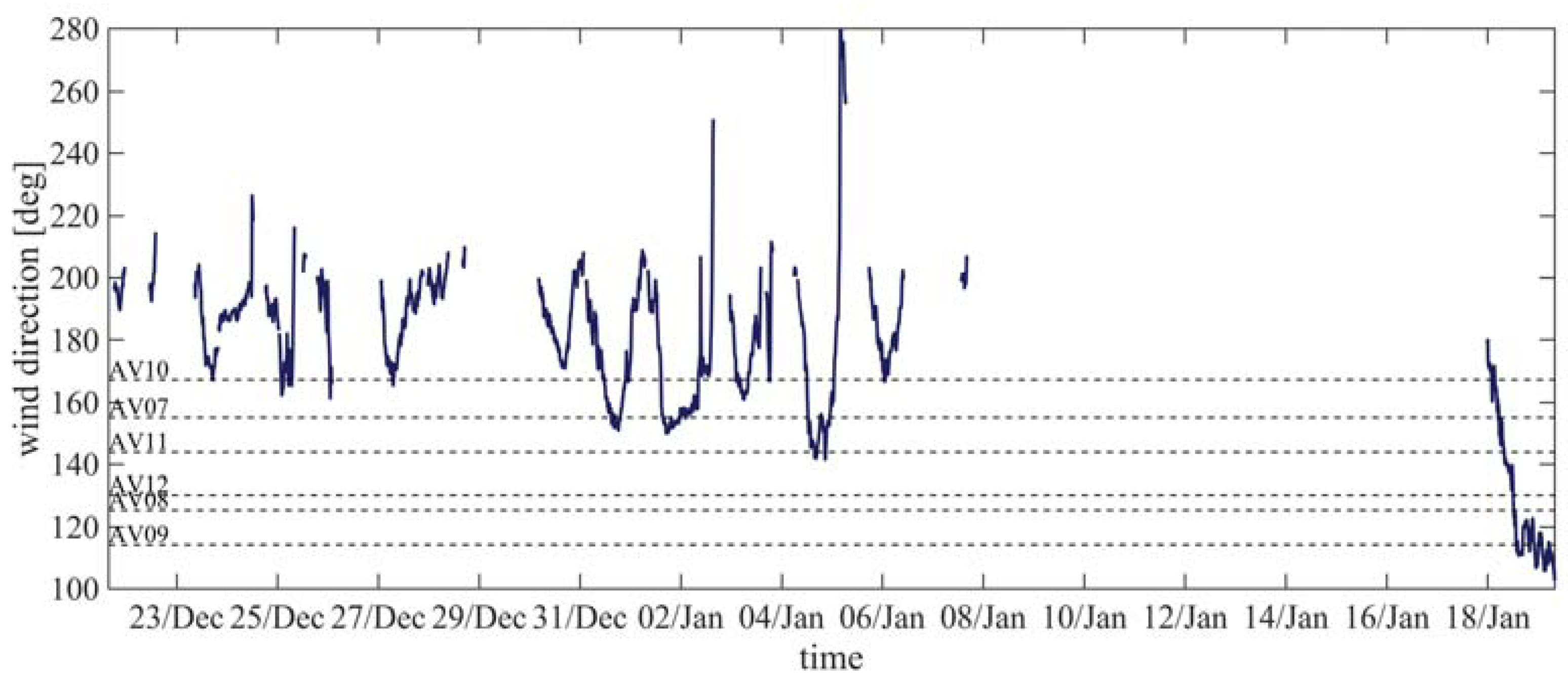
Figure 9.
Time series of the 10 min averaged wind direction measured by the ultrasonic anemometer from 21.12.2013 15:35 h (UTC) till 19.01.2014 7:55 h (UTC). Gaps in the plot demonstrate unavailability of LiDAR data. Horizontal lines indicate the wind direction of possible wake shading of the anemometer on FINO1 based on geometrical correlations.
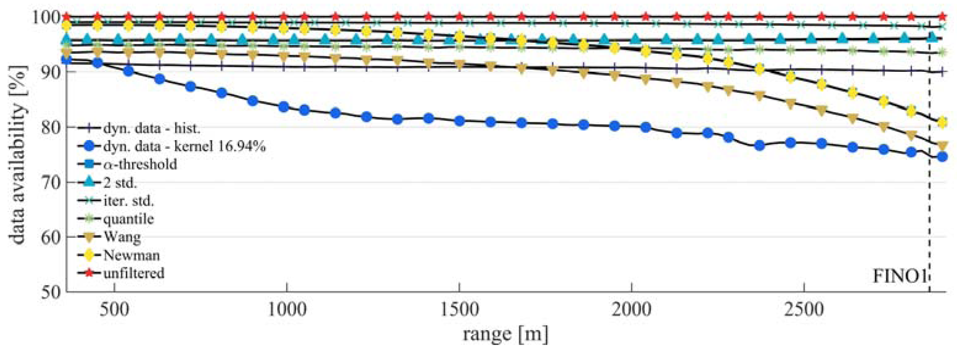
Figure 10.
Data availability of staring mode measurements for different filter methods. (a) time dependent behaviour for range at 2864 m and (b) averaged data availability over all ranges. The dashed line marks the distance of the anemometer at FINO1.
Figure 10.
Data availability of staring mode measurements for different filter methods. (a) time dependent behaviour for range at 2864 m and (b) averaged data availability over all ranges. The dashed line marks the distance of the anemometer at FINO1.
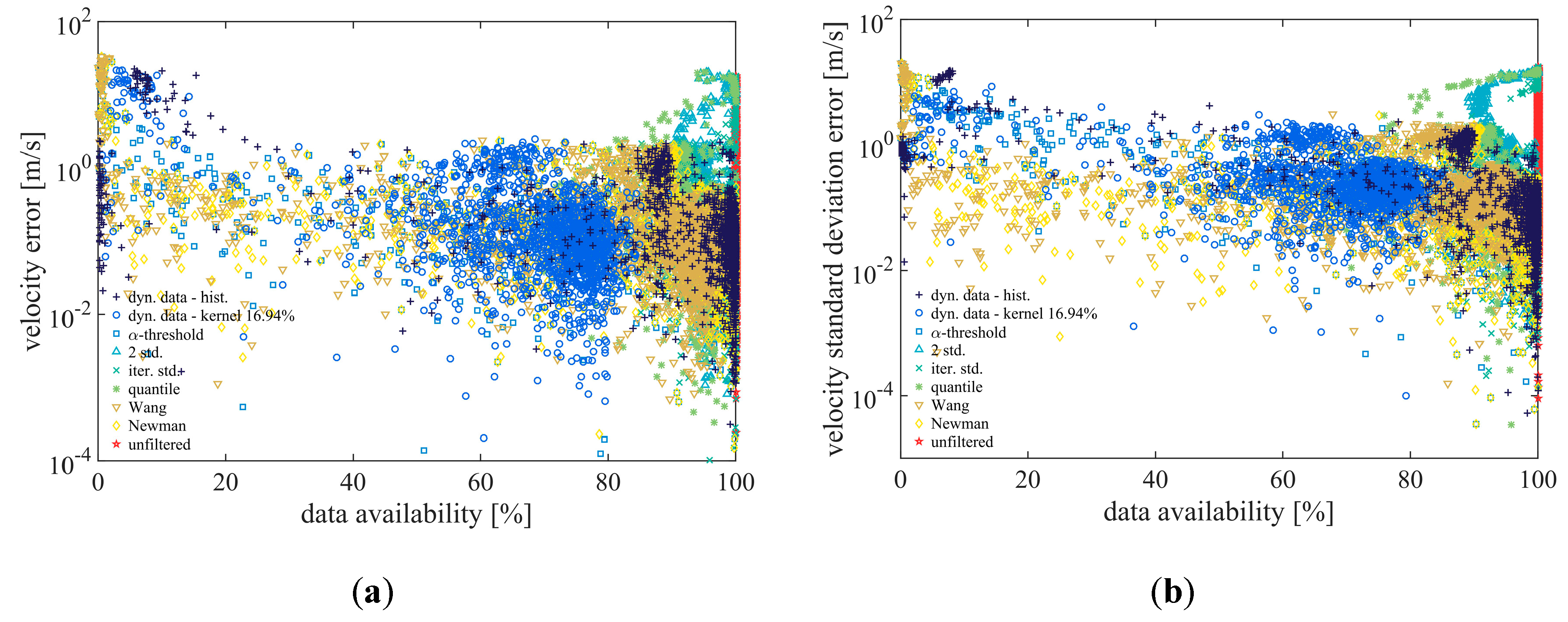
Figure 11.
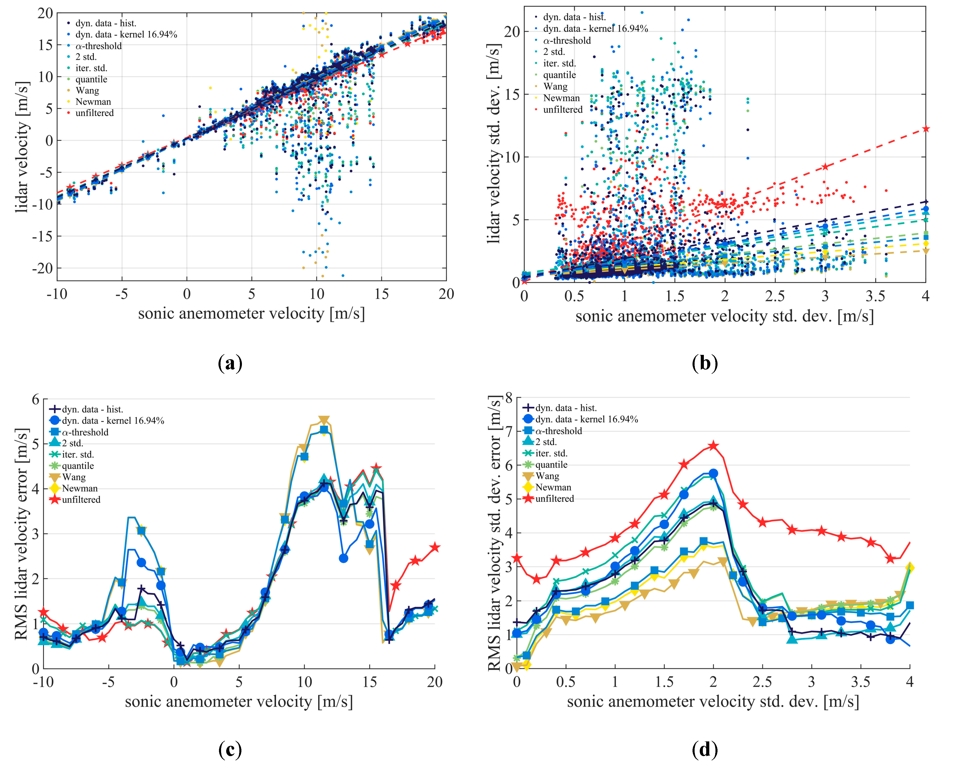
Absolute error of staring mode measurements in dependency of data availability. Markers represent 10 min values of (a) the velocity error and (b) the velocity standard deviation.
Figure 11.
Absolute error of staring mode measurements in dependency of data availability. Markers represent 10 min values of (a) the velocity error and (b) the velocity standard deviation.
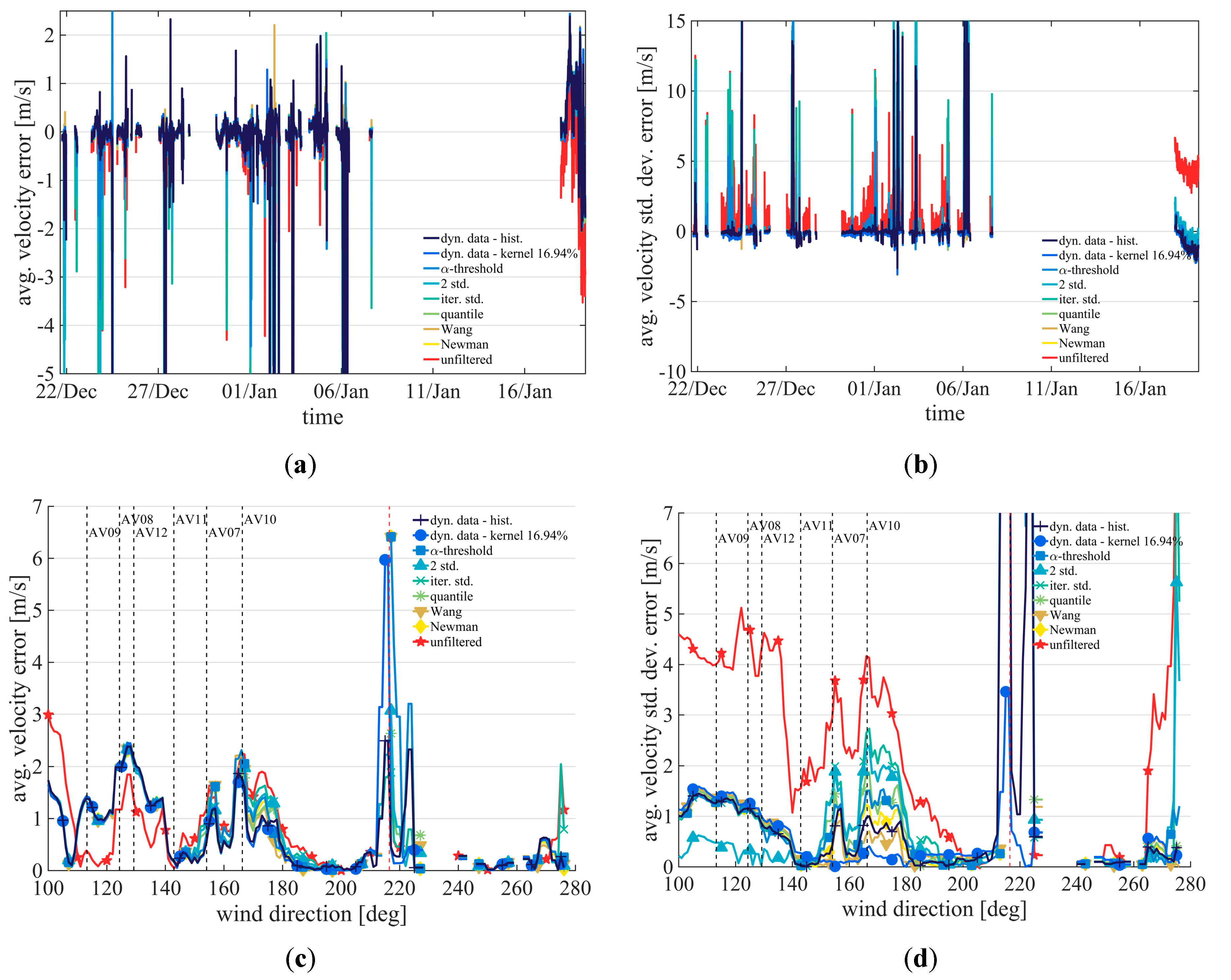
Figure 12.
Behaviour of the 10 min averaged filtered staring mode measurements of (a) the projected wind speed over time; (b) the standard deviation over time; (c) average wind speed error over wind direction; (d) average standard deviation error over wind direction. Vertical dashed lines indicate the wind direction of possible wake shading of the anemometer on FINO1 based on geometrical correlations.
Figure 13.
Behaviour of the 10 min averaged filtered staring mode measurements of (a) the projected wind speed over time, (b) the standard deviation over time, (c) average wind speed error over time, (d) standard deviation error over time.
Figure 13.
Behaviour of the 10 min averaged filtered staring mode measurements of (a) the projected wind speed over time, (b) the standard deviation over time, (c) average wind speed error over time, (d) standard deviation error over time.
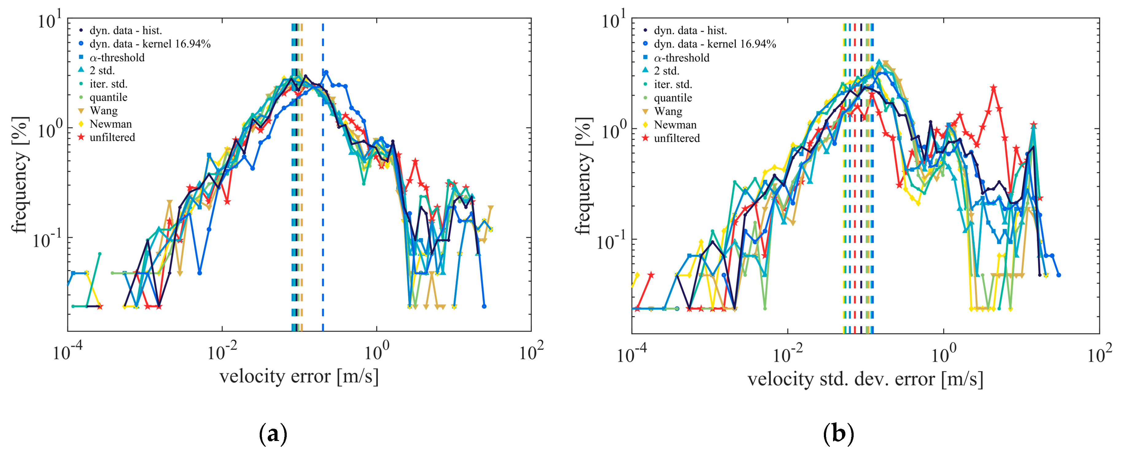
Figure 14.
Histogram in double logarithmic scaling with exponential increasing bin width of the (a) absolute average velocity error and (b) the absolute velocity standard deviation error. Vertical dashed lines indicate the centre of a fitted Gaussian curve.
Figure 14.
Histogram in double logarithmic scaling with exponential increasing bin width of the (a) absolute average velocity error and (b) the absolute velocity standard deviation error. Vertical dashed lines indicate the centre of a fitted Gaussian curve.
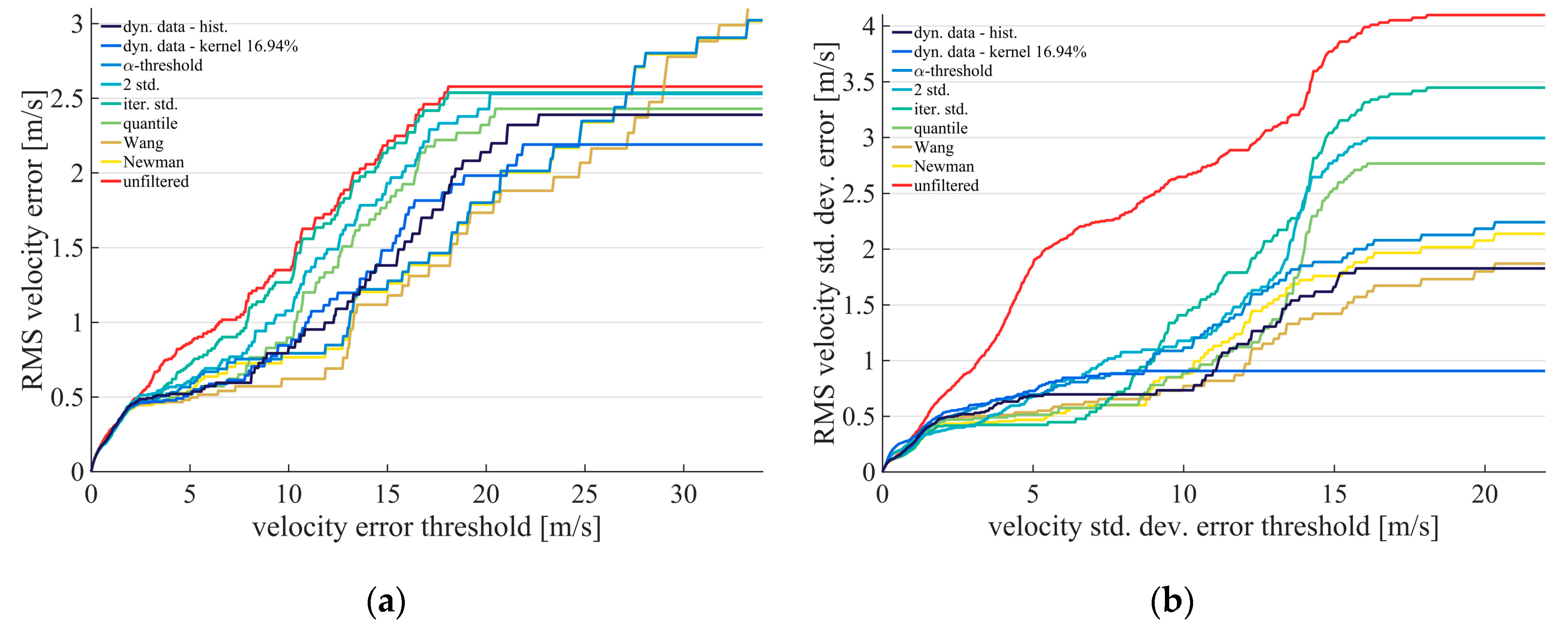
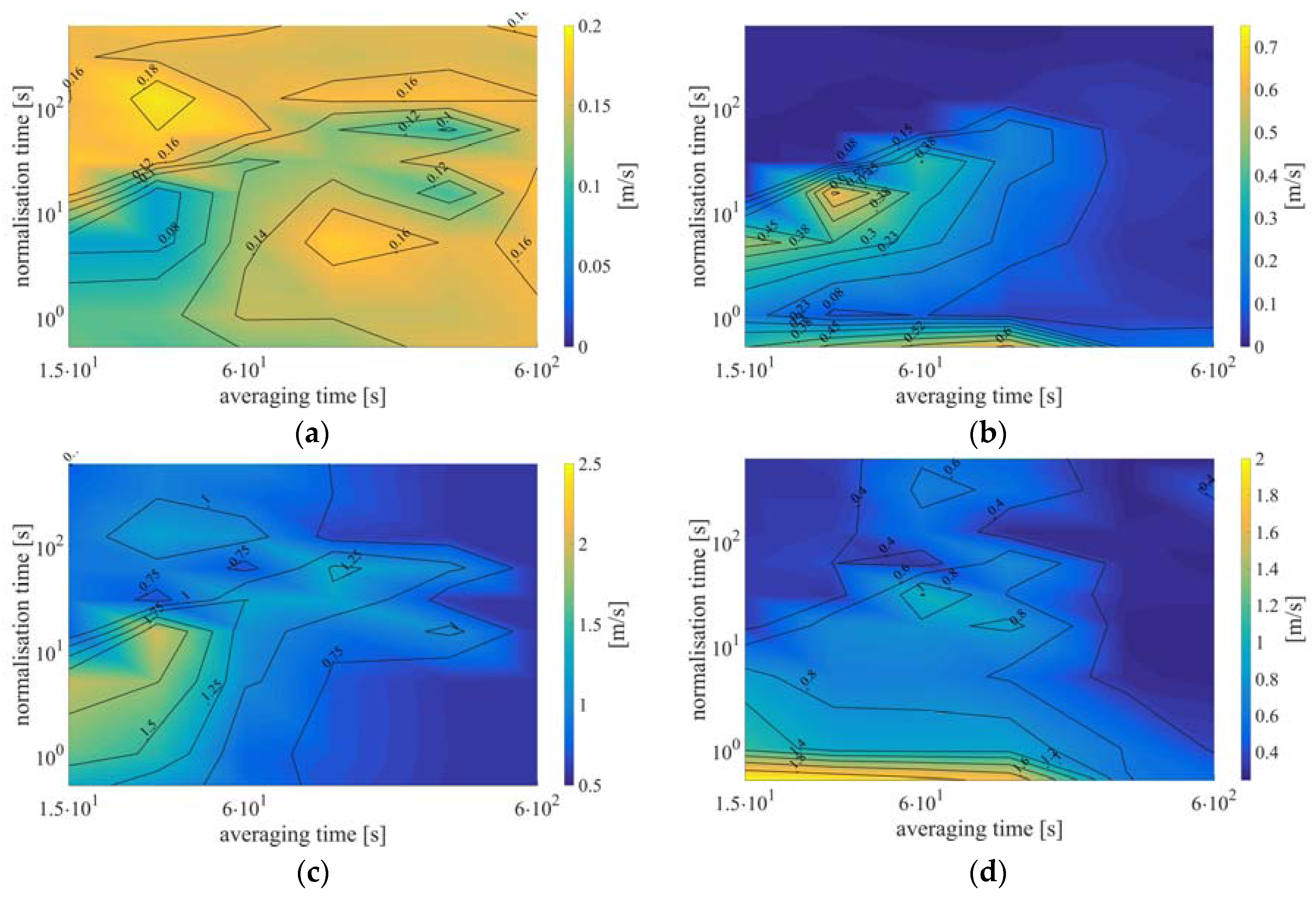
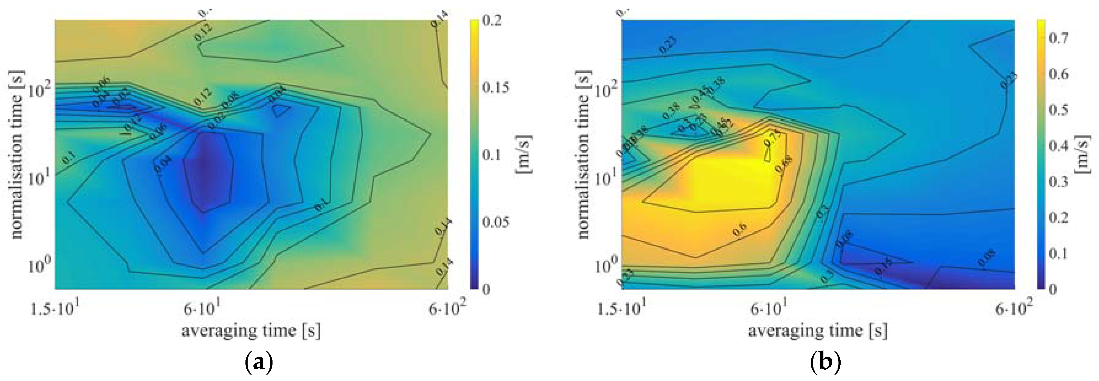
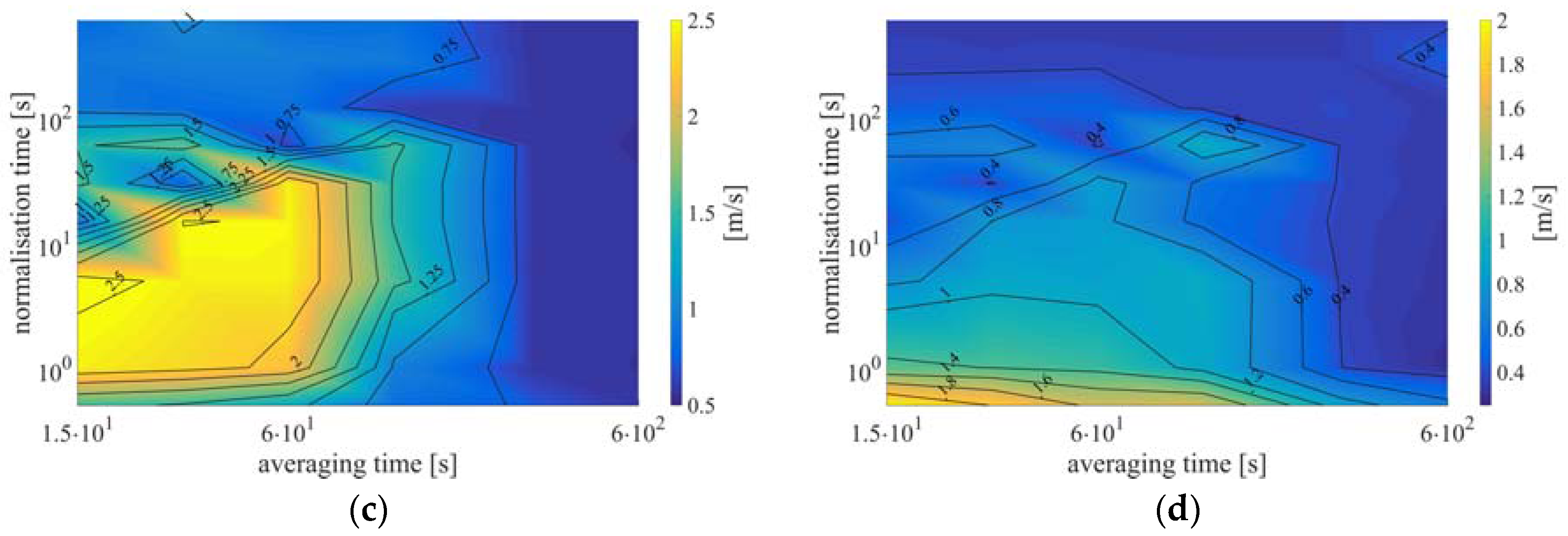
Figure 15.
Influence of maximum error threshold to the resulting error (a) RMS velocity error over velocity error threshold and (b) RMS velocity standard deviation error over velocity standard deviation error threshold.
Figure 15.
Influence of maximum error threshold to the resulting error (a) RMS velocity error over velocity error threshold and (b) RMS velocity standard deviation error over velocity standard deviation error threshold.
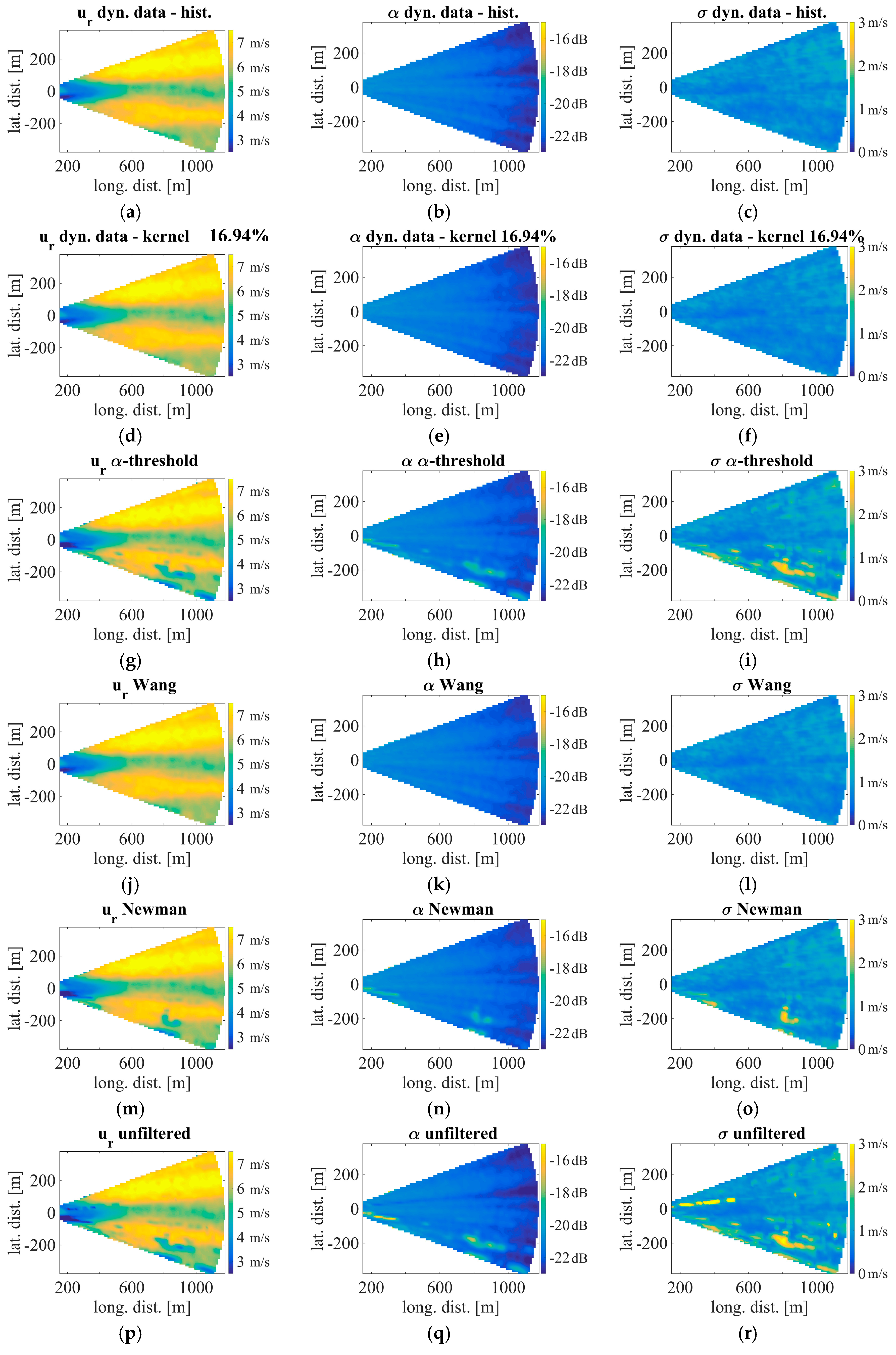
Figure 16.
Influence of different filtering methods on a 10 min averaged horizontal LiDAR scans. (1st column) radial speed, (2nd column) CNR mapping, (3rd column) standard deviation of radial speed. (a–c) histogram-based dynamic data filter, (d–f) Gaussian kernel based dynamic data filter, (g–i) CNR-threshold filter, (j–l) combined filter approach by Wang et al. (m–o) combined filter approach by Newman et al. (p–r) unfiltered.
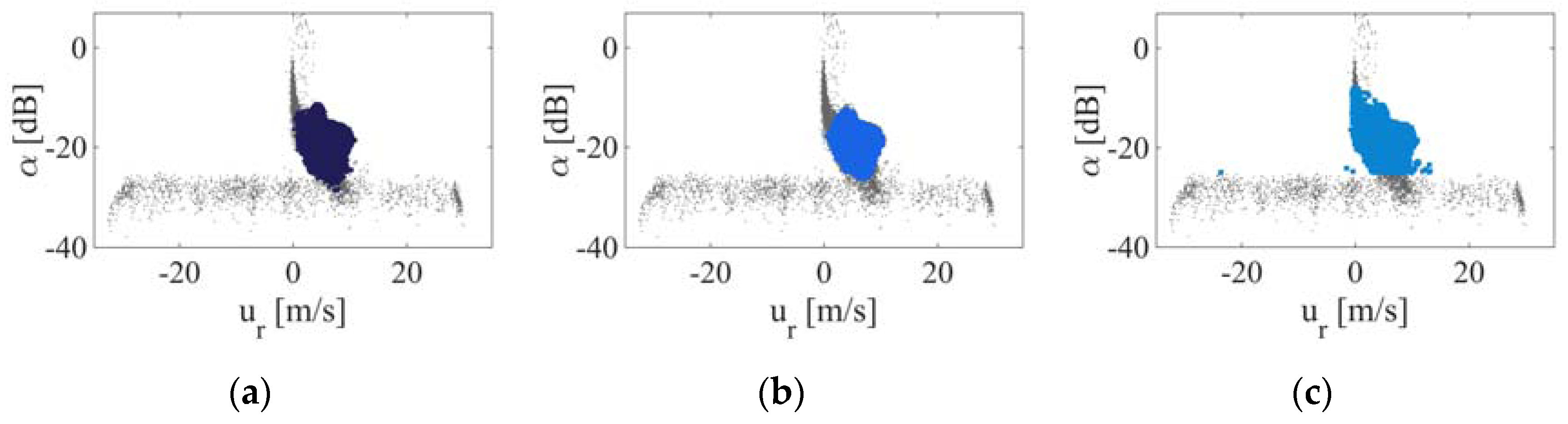
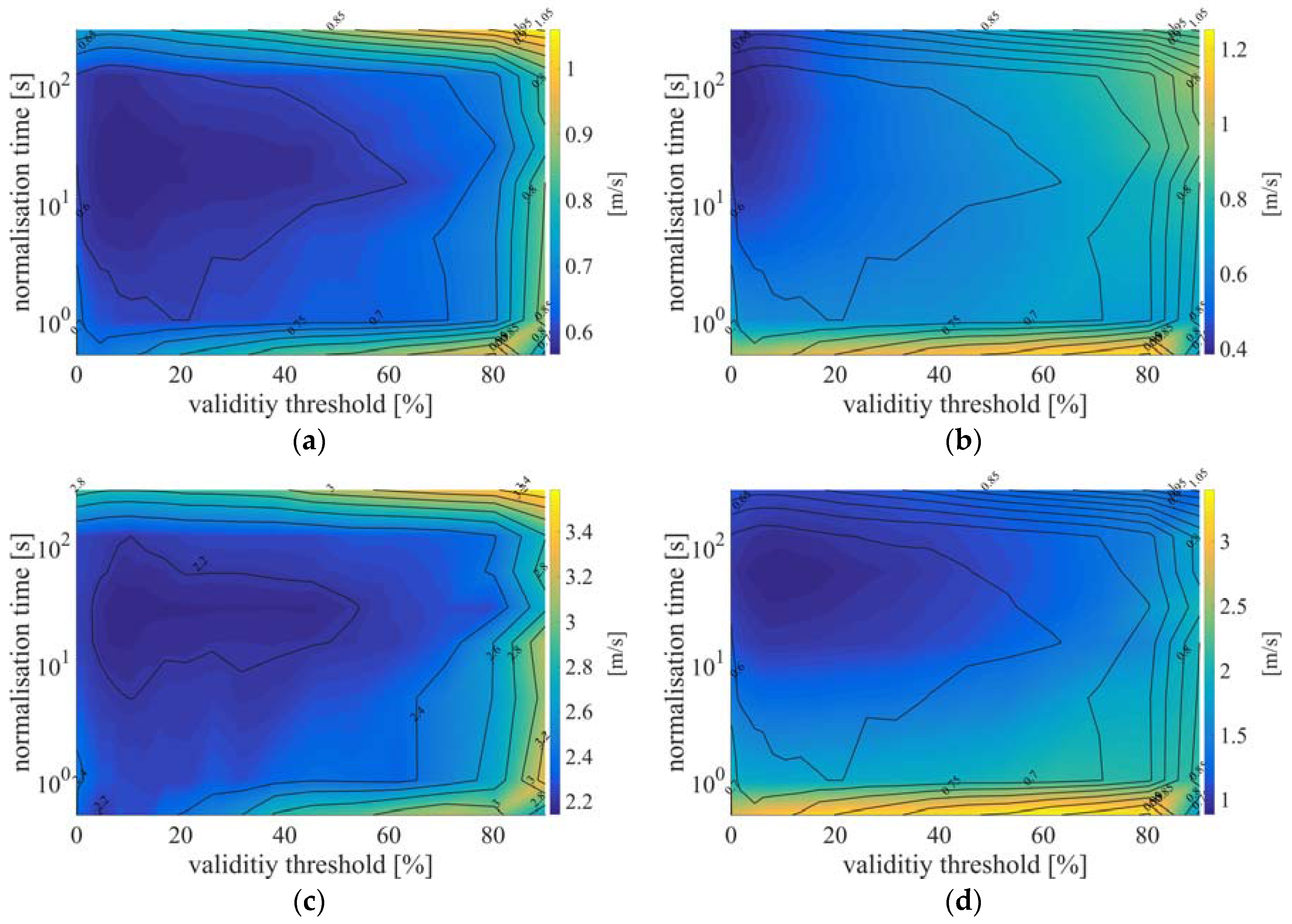
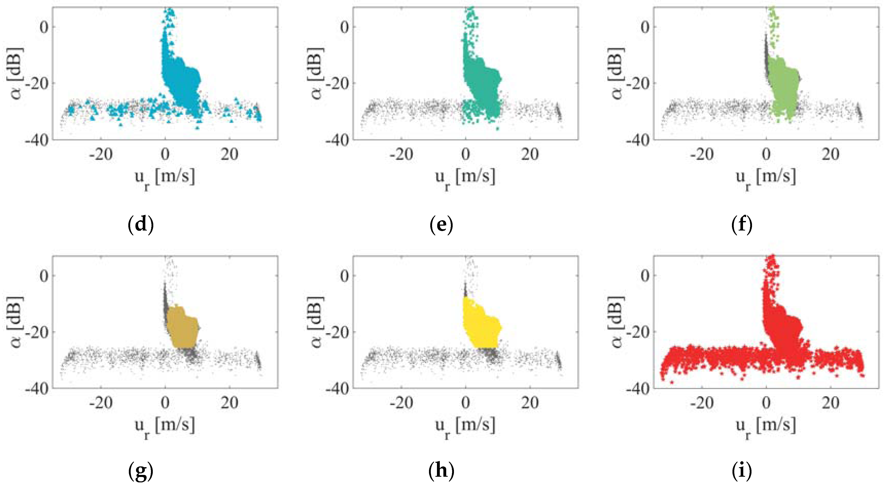
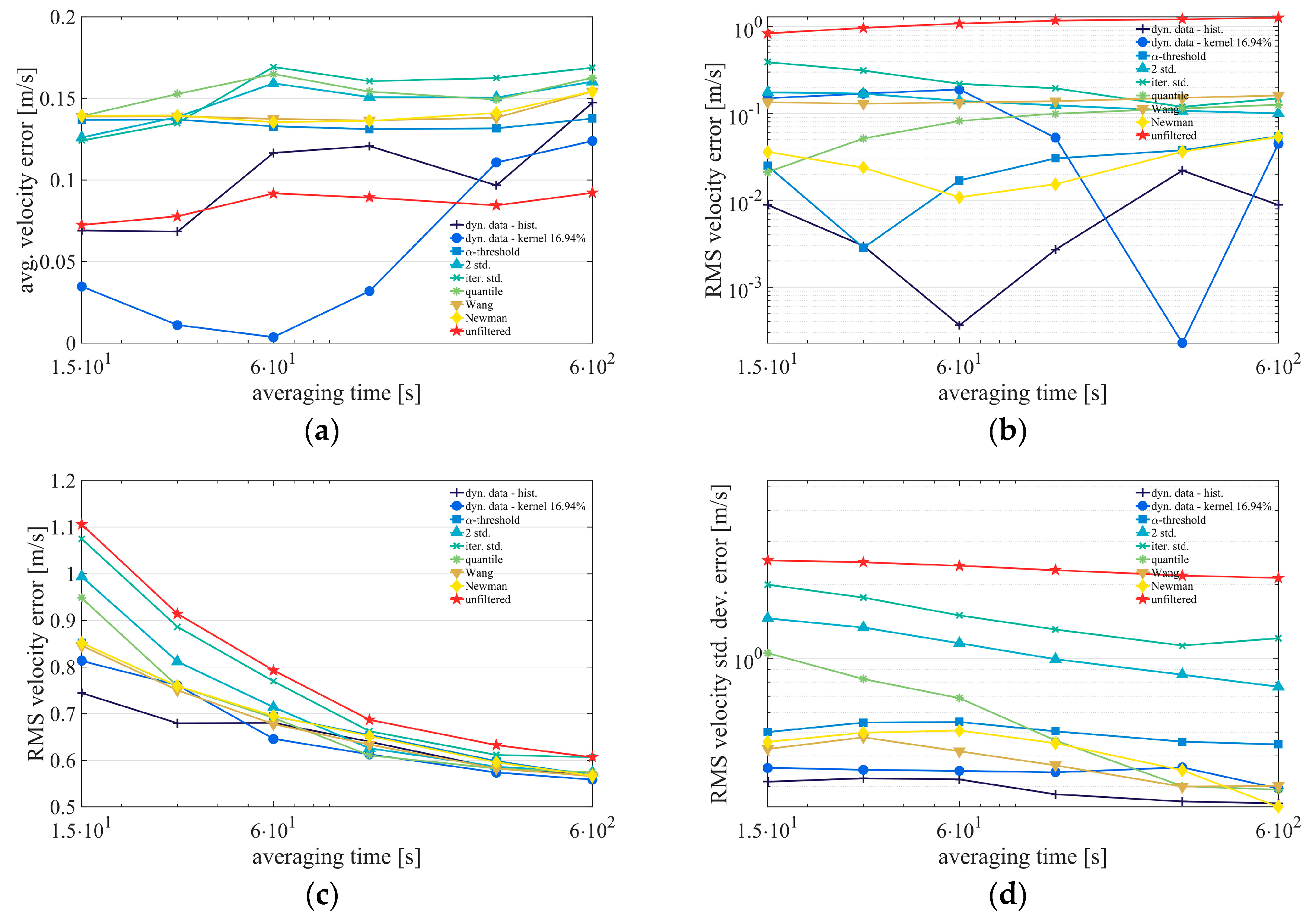
Figure 17.
Results of application of different filtering methods in the diagram. (a) histogram-based dynamic data filter, (b) Gaussian kernel based dynamic data filter, (c) CNR-threshold filter, (d) two sigma standard deviation filter, (e) iterative standard deviation filter, (f) interquartile-range, (g) combined filter approach by Wang et al. (h) combined filter approach by Newman et al. (i) no filtering.
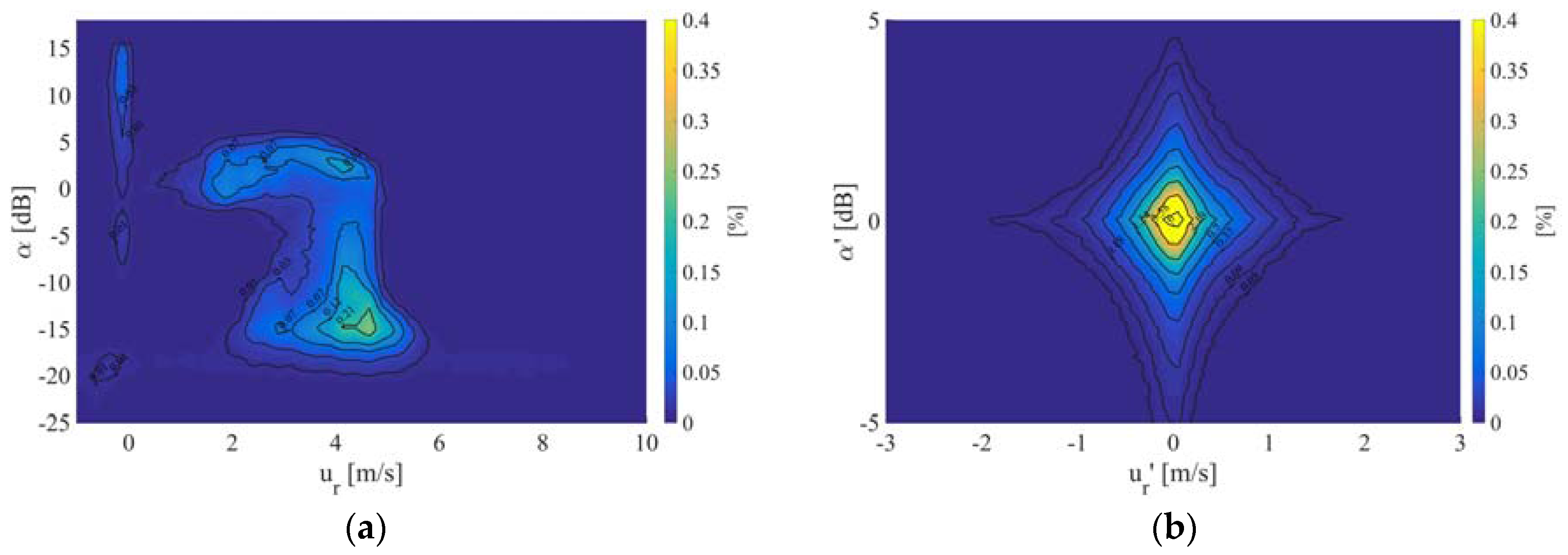
Figure 18.
Visualisation of the data density distribution of Stream Line XR PPI data from 31.10.2016 00:00 h (UTC) till 31.10.2016 00:30 h (UTC) in (a) diagram and (b) in the normalised reference frame.
Figure 18.
Visualisation of the data density distribution of Stream Line XR PPI data from 31.10.2016 00:00 h (UTC) till 31.10.2016 00:30 h (UTC) in (a) diagram and (b) in the normalised reference frame.
Table 1.
Comparison of different filtering methods applied on staring mode measurements from 21.12.2013 15:35 h (UTC) till 19.01.2014 7:55 h (UTC) for all wind directions.
Table 1.
Comparison of different filtering methods applied on staring mode measurements from 21.12.2013 15:35 h (UTC) till 19.01.2014 7:55 h (UTC) for all wind directions.
| | Avg. Availability FINO1 | Avg. Availability All Ranges | Abs. Avg. Velocity Error | RMS Velocity Error | Abs. Avg. Velocity Std. Dev. Error | RMS Velocity Std. Dev. Error |
|---|
| Dyn. data histogram | 90.0% | 90.4% | 0.34 m/s | 2.38 m/s | 0.14 m/s | 1.82 m/s |
| Dyn. data Gauss. kernel | 75.1% | 78.2% | 0.30 m/s | 2.10 m/s | 0.18 m/s | 0.90 m/s |
| CNR threshold | 81.9% | 87.6% | 0.45 m/s | 3.02 m/s | 0.36 m/s | 2.24 m/s |
| Std. dev. two sigma | 96.2% | 95.9% | 0.49 m/s | 2.50 m/s | 0.73 m/s | 3.00 m/s |
| Iterative std. dev. | 98.1% | 98.5% | 0.54 m/s | 2.54 m/s | 0.79 m/s | 3.45 m/s |
| Quartile filter | 93.5% | 94.0% | 0.40 m/s | 2.42 m/s | 0.35 m/s | 2.77 m/s |
| Combined Wang | 77.5% | 83.0% | 0.40 m/s | 3.10 m/s | 0.00 m/s | 1.87 m/s |
| Combined Newman | 81.8% | 87.5% | 0.42 m/s | 3.02 m/s | 0.20 m/s | 2.14 m/s |
| No filter | 100% | 100% | 0.76 m/s | 2.58 m/s | 2.17 m/s | 4.10 m/s |
Table 2.
Correlations and residuals of the linear regression between the ultrasonic anemometer and the LiDAR for the velocity and the standard deviation of the velocity. From 21.12.2013 15:35 h (UTC) till 19.01.2014 7:55 h (UTC) for all wind directions.
Table 2.
Correlations and residuals of the linear regression between the ultrasonic anemometer and the LiDAR for the velocity and the standard deviation of the velocity. From 21.12.2013 15:35 h (UTC) till 19.01.2014 7:55 h (UTC) for all wind directions.
| | Dyn. Data Hist. | Dyn. Data Gauss. | CNR Thres-hold | Std. Dev. | Iter. Std | Quartile | Wang | Newman | Unfiltered |
|---|
| Velocity | | | | | | | | | |
| Reg. slope | 0.92 | 0.95 | 0.96 | 0.92 | 0.91 | 0.93 | 0.97 | 0.97 | 0.86 |
| Offset [m/s] | 0.31 | 0.26 | 0.22 | 0.33 | 0.32 | 0.32 | 0.22 | 0.22 | 0.44 |
| R2 | 0.85 | 0.84 | 0.90 | 0.83 | 0.79 | 0.85 | 0.90 | 0.90 | 0.78 |
| Velocity std. dev. | | | | | | | | | |
| Reg. slope | 1.50 | 1.39 | 0.73 | 1.27 | 1.05 | 0.86 | 0.50 | 0.62 | 3.04 |
| Offset [m/s] | 0.42 | 0.33 | 0.63 | 0.45 | 0.74 | 0.49 | 0.50 | 0.58 | 0.08 |
| R2 | 0.06 | 0.04 | 0.02 | 0.04 | 0.02 | 0.02 | 0.01 | 0.01 | 0.15 |
Table 3.
Most probable velocity and standard deviation error of fitted double log-normal distribution to 10 min error histogram.
Table 3.
Most probable velocity and standard deviation error of fitted double log-normal distribution to 10 min error histogram.
| | Dyn. Data Hist. | Dyn. Data Gauss. | CNR Thres-hold | Std. Dev. | Iter. Std | Quartile | Wang | Newman | Unfiltered |
|---|
| Velocity [m/s] | 0.09 | 0.20 | 0.09 | 0.09 | 0.09 | 0.10 | 0.11 | 0.09 | 0.11 |
| Vel. std. dev. [m/s] | 0.09 | 0.12 | 0.06 | 0.12 | 0.06 | 0.10 | 0.11 | 0.06 | 0.07 |


