Abstract
Marginal Fisher analysis (MFA) exploits the margin criterion to compact the intraclass data and separate the interclass data, and it is very useful to analyze the high-dimensional data. However, MFA just considers the structure relationships of neighbor points, and it cannot effectively represent the intrinsic structure of hyperspectral imagery (HSI) that possesses many homogenous areas. In this paper, we propose a new dimensionality reduction (DR) method, termed local geometric structure Fisher analysis (LGSFA), for HSI classification. Firstly, LGSFA uses the intraclass neighbor points of each point to compute its reconstruction point. Then, an intrinsic graph and a penalty graph are constructed to reveal the intraclass and interclass properties of hyperspectral data. Finally, the neighbor points and corresponding intraclass reconstruction points are used to enhance the intraclass-manifold compactness and the interclass-manifold separability. LGSFA can effectively reveal the intrinsic manifold structure and obtain the discriminating features of HSI data for classification. Experiments on the Salinas, Indian Pines, and Urban data sets show that the proposed LGSFA algorithm achieves the best classification results than other state-of-the-art methods.
1. Introduction
Hyperspectral imagery (HSI) is captured by remote sensors recording the reflectance values of electromagnetic wave, and each pixel in HSI is a spectral curve containing hundreds of bands from visible to near-infrared spectrum [1,2,3,4]. The HSI can offer much richer information, and it can discriminate the subtle differences in different land cover types [5,6]. HSI plays a significant role in the application of anomaly detection, agricultural production, disaster warning, and land cover classification [7,8,9]. However, the traditional classification methods commonly cause the Hughes phenomena because of the high dimensional characteristics in HSI [10,11,12]. Therefore, a huge challenge for HSI processing is to reduce the dimensionality of high-dimensional data with some valuable intrinsic information preserved.
Dimensionality reduction (DR) is commonly applied to reduce the number of bands in HSI and obtain some desired information [13,14,15]. A large number of methods have been designed for DR of HSI. Principal component analysis (PCA) has been widely used for high-dimensional data, and it applies orthogonal projection to maximize data variance [16]. To improve the noise robustness of PCA, the researchers proposed minimum noise fraction (MNF) with noise variance [17]. MNF maximizes the signal-to-noise ratio to obtain the principal components, and it provides satisfactory results for HSI classification. However, PCA and MNF are unsupervised methods, and they restrain the discriminating power for HSI classification. To enhance the discriminating power, some supervised methods have been proposed. Linear discriminant analysis (LDA) is a traditional supervised method based on the mean vector and covariance matrix of classes, and it is defined by the maximization of between-class scatter and the minimization of within-class scatter [18]. However, LDA only involves features (where c is the class number of data), which may not obtain sufficient features for hyperspectral classification. To address this problem, the researchers proposed maximum margin criterion (MMC) [19] and local Fisher discriminant analysis (LFDA) [20,21] for obtaining enough features, while these methods originate from the theory of statistics and neglect the geometry properties of hyperspectral data.
Recently, the intrinsic manifold structure has been discovered in HSI [22]. Many manifold learning methods have been applied to obtain the manifold properties from high-dimensional data [23,24,25,26]. Such methods include isometric mapping (Isomap) [27], Laplacian eigenmaps (LE) [28] and locally linear embedding (LLE) [29]. The Isomap method adopts the geodesic distances between data points to reduce the dimensionality of data. The LLE method preserves the local linear structure of data in a low-dimensional space. The LE method applies the Laplacian matrix to reveal the local neighbor information of data. However, these manifold learning algorithms cannot obtain explicit projection matrix that can map a new sample into the corresponding low-dimensional space. To overcome this problem, locality preserving projections (LPP) [30] and neighborhood preserving embedding (NPE) [31] were proposed to approximately linearize the LE and LLE algorithms, respectively. However, LPP and NPE are unsupervised DR methods that cannot perform good discriminating power in certain scenes.
To unify these methods, a graph embedding (GE) framework has been proposed to analyze the DR methods on the basis of statistics or geometry theory [32]. Many algorithms, such as PCA, LDA, LPP, ISOMAP, LLE and LE, can be redefined in this framework. The differences between these algorithms lie in the computation of the similarity matrix and the selection of the constraint matrix. With this framework, marginal Fisher analysis (MFA) is developed for DR. MFA designs an intrinsic graph to characterize the intraclass compactness and a penalty graph to characterize the interclass separability. The intrinsic graph represents the similarity of intraclass points from the same class, while the penalty graph illustrates the connected relationship of interclass points that belongs to different classes. MFA can reveal the intraclass and interclass manifold structures. However, it only considers the structure relationships of pairwise neighbor points, which may not effectively represent the intrinsic structure relationship of HSI with a larger number of homogenous areas [33,34]. Therefore, MFA may not obtain good discriminating power for HSI classification.
To address this problem, we propose a new DR method called local geometric structure Fisher analysis (LGSFA) in this paper. Firstly, it reconstructs each point with intraclass neighbor points. In constructing the intrinsic graph and the penalty graph, it compacts the intraclass neighbor points and corresponding reconstruction points, and it simultaneously separates the interclass neighbor points and corresponding reconstruction points. LGSFA can better represent the intrinsic manifold structures, and it also enhances the intraclass compactness and the interclass separability of HSI data. Experimental results on three real hyperspectral data sets show that the proposed LGSFA algorithm is more effective than other DR methods to extract the discrimination features for HSI classification.
The rest of this paper is organized as follows. Section 2 briefly reviews the theories of GE and MFA. Section 3 details our proposed method. Experimental results are presented in Section 4 to demonstrate the effectiveness of the proposed method. Finally, Section 5 provides some concluding remarks and suggestions for future work.
2. Related Works
Let us suppose a data set , where n and D are the number of samples and bands in HSI, respectively. The class label of is denoted as , where c is the number of classes. The low-dimensional data is represented as , where d is the embedding dimensionality. Y is represented by with projection matrix .
2.1. Graph Embedding
The graph embedding (GE) framework is used to unify most popular DR algorithms [32]. In GE, an intrinsic graph is constructed to describe some of the desirable statistical or geometrical properties of data, while a penalty graph is utilized to represent some of the unwanted characteristics of data [35]. The intrinsic graph and penalty graph are two undirected weighted graphs with the weight matrices and , where X denotes the vertex set. Weight reveals the similarity characteristic of the edges between vertices i and j in , while weight refers to the dissimilarity structure between vertices i and j in .
The purpose of graph embedding is to project each vertex of the graph into a low-dimensional space that preserves the similarity between the vertex pairs. The objective function of the graph embedding framework is formulated as follows:
where h is a constant, H is a constraint matrix defined to find the non-trivial solution of (1), and L is the Laplacian matrix of graph G. Typically, is the Laplacian matrix of graph , that is, . Laplacian matrices L and can be reformulated as
where diag(•) denotes that a vector is transformed as a diagonal matrix.
2.2. Marginal Fisher Analysis
MFA constructs an intrinsic graph and a penalty graph. The intrinsic graph connects each point with its neighbor points from the same class to characterize the intraclass compactness, while the penalty graph connects the marginal points from different classes to characterize the interclass separability.
In intrinsic graph , each data point is connected with the intraclass neighbor points that are from the same class. The similarity weight between and is defined as
where denotes the intraclass neighbor points of . The intraclass neighbor points denotes the intraclass similarity relationship of data that should be preserved in low-dimensional embedding space.
For penalty graph , is connected with the interclass neighbor points that are from different classes. The penalty weight between and is set as
where denotes the interclass neighbor points of . The interclass neighbor points represents the interclass similarity relationship of data that should be avoided in low-dimensional embedding space.
To enhance intraclass compactness and interclass separability, the optimal projection matrix V can be obtained with the following optimization problem:
3. Local Geometric Structure Fisher Analysis
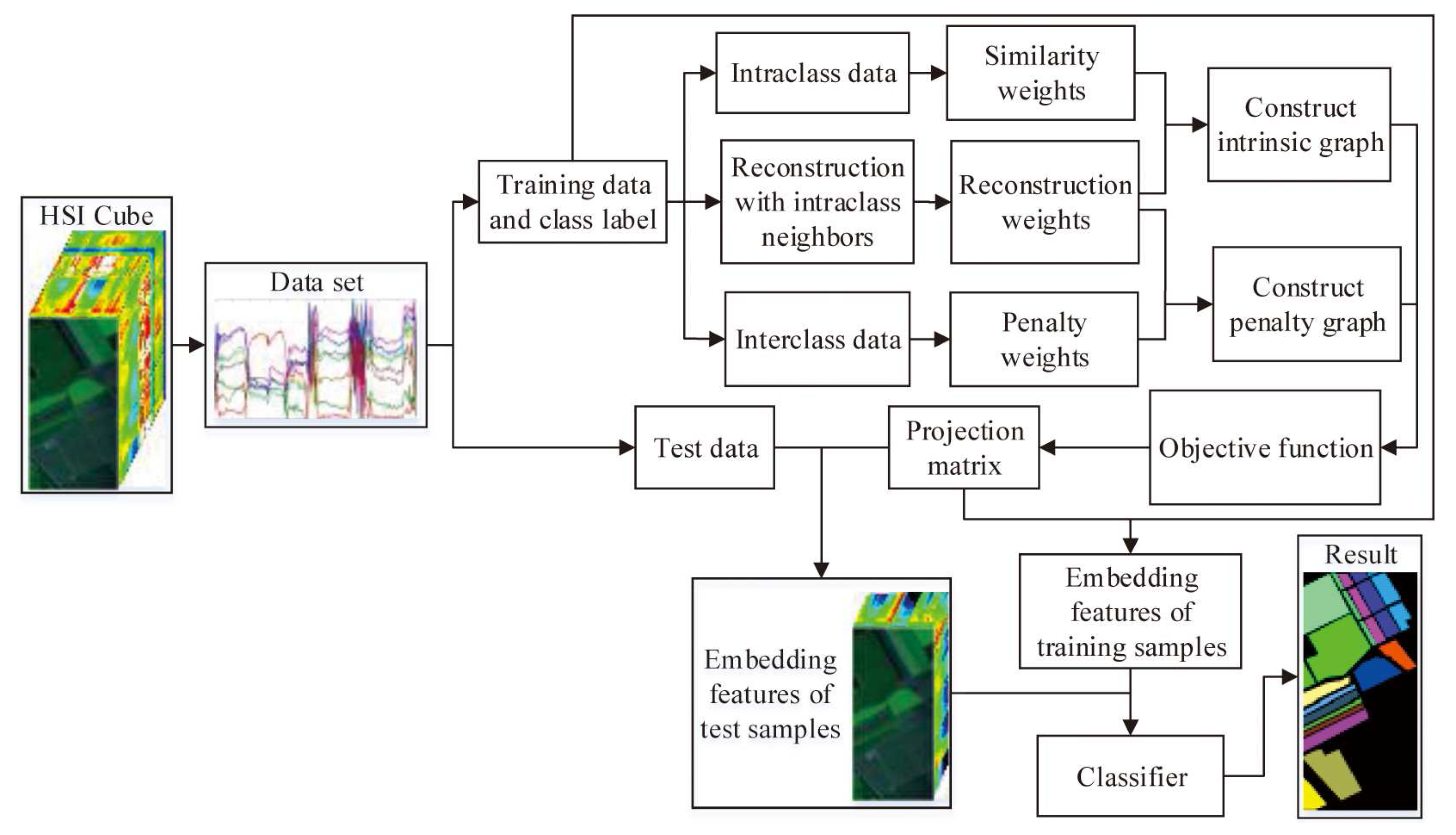
To effectively reveal the intrinsic manifold structure of hyperspectral data, a local geometric structure Fisher analysis (LGSFA) method was proposed based on MFA. This method computes the reconstruction point of each point with its intraclass neighbor points. Then, it uses the intraclass and interclass neighbor points to construct an intrinsic graph and a penalty graph, respectively. With the intrinsic graph, it utilizes the intraclass neighbor points and corresponding reconstruction points to compact the data points from the same class. With the penalty graph, it adopts the interclass neighbor points and corresponding reconstruction points to separate the data points from different classes. LGSFA further improves both the intraclass compactness and the interclass separability of hysperspectral data, and it can obtain better discriminating features to enhance the classification effect. The process of the LGSFA method is shown in Figure 1.
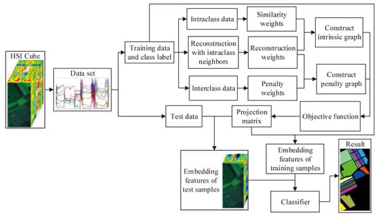
Figure 1.
Process of the proposed LGSFA method.
Each point can be reconstructed with its neighbor points from the same class. The reconstruction weight is computed by minimizing the sum of reconstruction errors
where is the reconstruction weight between and . If is the intraclass neighbor points of , or , and .
With some mathematical operations, (7) can be reduced as
where , is the ith intraclass neighbor point of .
Thus, (7) can be denoted as
According to the method of Lagrangian multipliers, the optimization solution is
where . After obtaining , the reconstruction point of can be represented as .
To reveal the manifold structure of hyperspectral data, we construct an intrinsic graph to characterize the similarity properties of data from the same class and a penalty graph to stress the dissimilarity of data from different classes. The similarity weight between and of the intrinsic graph are defined as
where .
For the penalty graph, the weights are represented as
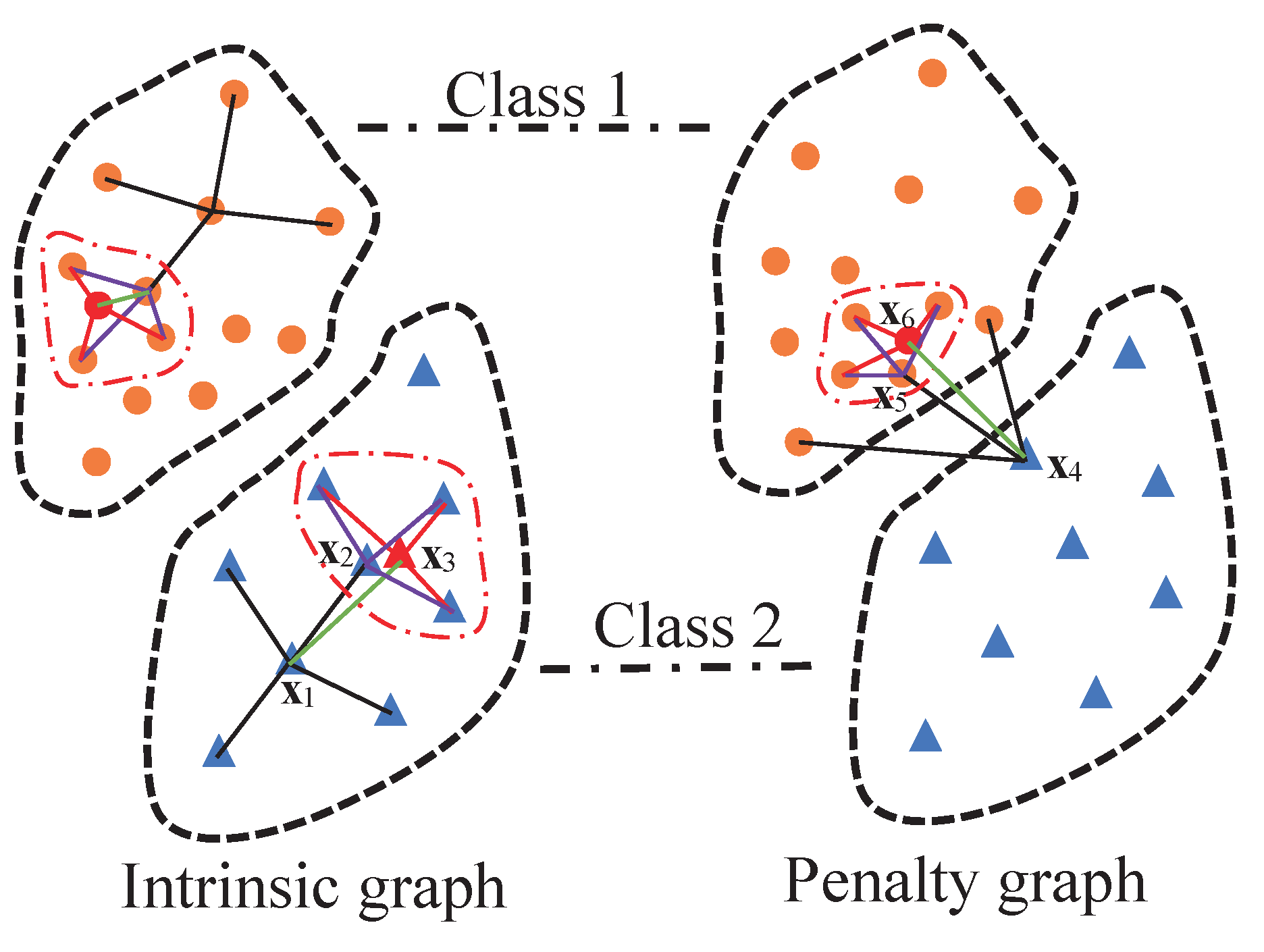
To illustrate the graph construction of the LGSFA method, an example is shown in Figure 2. In the intrinsic graph, point is the intraclass neighbor point of , and point is the reconstruction point of obtained by its intraclass neighbor points that are in the curve of dot dash line. In the penalty graph, point is the interclass neighbor point of , and point is the reconstruction point of . The intrinsic graph and the penalty graph are constructed on the basis of intraclass neighbor points, interclass neighbor points and corresponding reconstruction points. In these graphs, we consider the structure relationships not only between each point and its neighbor points but also between that point and the reconstruction points of its neighbor points. This process can effectively represent the intrinsic structure of HSI, and it can improve the compactness of data from the same class and the separability of data from different classes.
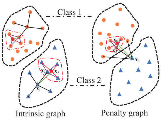
Figure 2.
Graph construction of the LGSFA method.
To enhance the intraclass compactness, we apply the intraclass neighbor points and corresponding reconstruction points to construct an objective function in a low-dimensional embedding space
In addition, we also construct an objective function with interclass neighbor points and corresponding reconstruction points to improve the interclass separability as follows:
where , , , , .
To obtain a projection matrix, the optimization problems of (16) and (17) can be changed into another form as follows:
According to the method of Lagrangian multipliers, the optimization problem is transformed to solve a generalized eigenvalue problem, i.e.,
The optimization projection matrix can be obtained by the d minimum eigenvalues of (19) corresponding eigenvectors. Then, the low-dimensional features can be formulated by
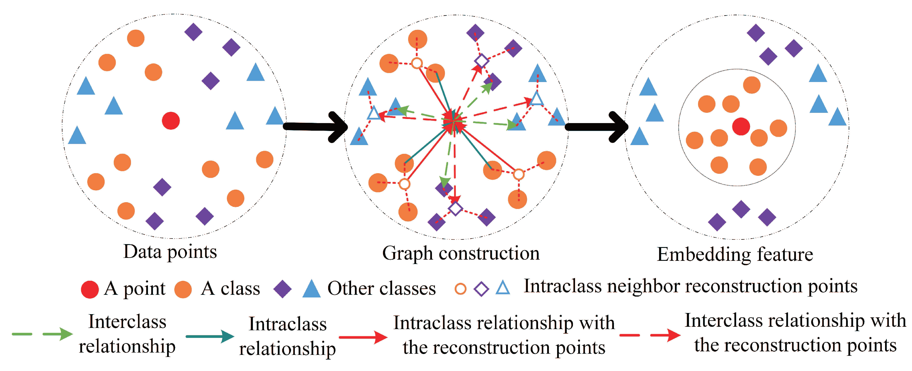
In summary, the proposed LGSFA method considers the neighbor points and corresponding reconstruction points to improve the intraclass compactness and the interclass separability of hyperspectral data. Therefore, it can effectively extract the discriminating feature for HSI classification. An example for the processing of LGSFA is shown in Figure 3.
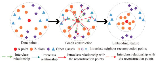
Figure 3.
An example for the processing of LGSFA.
According to Figure 3, the proposed LGSFA method applies the intraclass, interclass, and intraclass neighbor reconstruction relationships to enhance the compactness of data from the same class and the separability of data from different classes. The detailed steps of the proposed LGSFA method are shown in Algorithm 1.
According to the process in Algorithm 1, we adopt big O notation to analyze the computational complexity of LGSFA. The number of intraclass neighbors and interclass neighbors is denoted as and , respectively. The reconstruction weight matrix S is computed with the cost of . The intraclass weight matrix and the interclass weight matrix take and , respectively. The diagonal matrices and both cost . The intraclass manifold matrix and the interclass manifold matrix are both calculated with . The costs of and are both . It takes to solve the generalized eigenvalue problem of (19). For and , the total computational complexity of LGSFA is that mainly depends on the number of bands, training samples, and neighbor points.
| Algorithm 1 LGSFA |
|
4. Experimental Results and Discussion
We employed the Salinas, Indian Pines, and Urban HSI data sets to evaluate the proposed LGSFA method, and it was compared with some state-of-art DR algorithms.
4.1. Data Sets
Salinas data set: The HSI data set was collected by an airborne visible/infrared imaging spectrometer (AVIRIS) sensor over Salinas Valley, Southern California, in 1998. This data set has a geometric resolution of 3.7 m. The area possesses a spatial size of 512–217 pixels and 224 spectral bands from 400 nm to 2500 nm. Exactly 204 bands remained after the removal of bands 108–122, 154–167 and 224 as a result of dense water vapor and atmospheric effects. The data set contains sixteen land cover types. The scene in false color and its corresponding ground truth are shown in Figure 4.
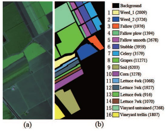
Figure 4.
Salinas hyperspectral image. (a) HSI in false color; (b) Ground truth.
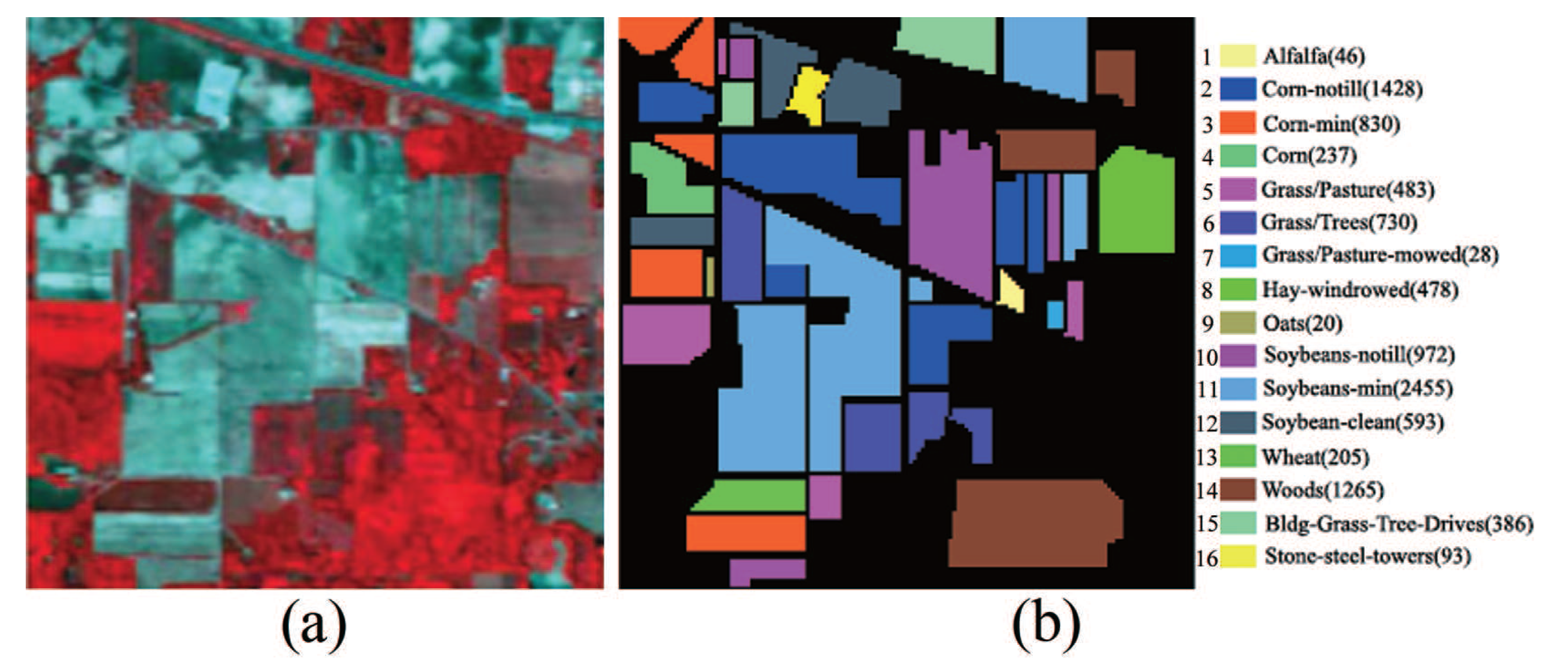
Indian Pines data set: This data set is a scene of the Northwest Indiana collected by the AVIRIS sensor in 1992. It consists of pixels and 220 spectral bands within the range of 375–2500 nm. Several spectral bands, including bands 104–108, 150–163 and 220, with noise and water absorption phenomena were removed from the data set, leaving a total of 200 radiance channels to be used in the experiments. Sixteen ground truth classes of interest are considered in the data set. The scene in false color and its corresponding ground truth are shown in Figure 5.
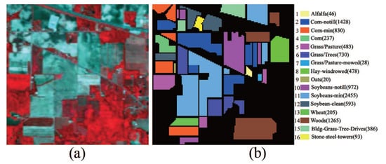
Figure 5.
Indian Pines hyperspectral image. (a) HSI in false color; (b) Ground truth.
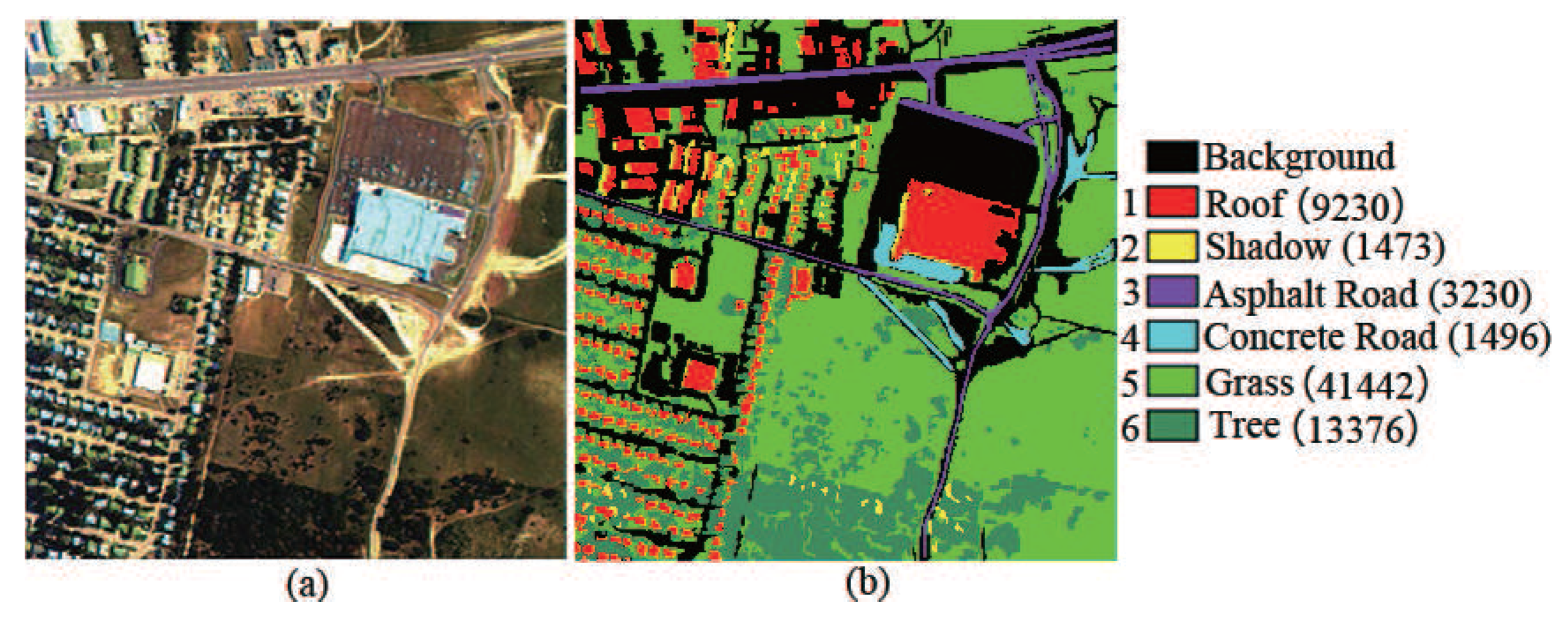
Urban data set: This data set was captured by the hyperspectral digital imagery collection experiment (HYDICE) sensor at the location of Copperas Cove, near Fort Hood, Texas, USA in October 1995. This data set is of size 307 × 307 pixels, and it is composed of 210 spectral channels with spectral resolution of 10 nm in the range from 400 to 2500 nm. After removing water absorption and low SNR bands, 162 bands were used for experiment. Six land cover types are considered in this data set. The scene in false color and its corresponding ground truth are shown in Figure 6.
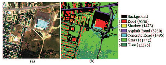
Figure 6.
Urban hyperspectral image. (a) HSI in false color; (b) Ground truth.
4.2. Experimental Setup
In each experiment, the data set was randomly divided into training and test samples. A dimensionality reduction method was applied to learn a low-dimensional space with the training samples. Then, all test samples were mapped into a low-dimensional space. After that, we employed the nearest neighbor (NN) classifier, the spectral angle mapper (SAM) and the support vector machine based on composite kernels (SVMCK) [36] to classify test samples. For NN, it depends on the nearest Euclidean distance to discriminate the class of test samples. For SAM, the class of test samples is obtained by the smallest spectral angle. For SVMCK, it is an extensional SVM and simultaneously applies the spatial and spectral information of HSI to discriminate the class of test samples. Finally, the average classification accuracy (AA), the overall classification accuracy (OA), and the Kappa coefficient (KC) were adopted to evaluate the performance of each method. To robustly evaluate the results, the experiments were repeated 10 times in each condition, and we displayed the average classification accuracy with standard deviation (STD).
In the experiment, we compared the proposed LGSFA algorithm with the Baseline, PCA, NPE, LPP, sparse discriminant embedding(SDE) [13], LFDA, MMC and MFA methods, where the Baseline method represents that a classifier was directly used to classify the test samples without DR. To achieve optimal results for each method, we adopted cross-validation to obtain the optimal parameters of each method. For LPP, NPE and LFDA, the number of neighbor points was optimistically set to 9. For SDE, we set the error tolerances to 5. For MFA and LGSFA, we set the intraclass neighbor and interclass neighbor , where is a positive integer. The values of k and were set to 9 and 20, respectively. For SVMCK, we used a weighted summation kernel, which generated the best classification performance compared with other composite kernels [36]. The spatial information was represented by the mean of pixels in a small neighborhood, and the RBF kernel was used with the LibSVM Toolbox [37]. The penalty term C and the RBF kernel width were selected by a grid search with a given set . The spatial window of size in the SVMCK classifier was set to for Indian Pines and Salinas data sets, and for Urban data set. The embedding dimension was 30 for all the DR methods. All the experiments were performed on a personal computer with i7-4790 central processing unit, 8-G memory, and 64-bit Windows 10 using MATLAB 2013b.
4.3. Two-Dimension Embedding
In this section, we use the Indian Pines data set to analyze the two-dimension embedding of the proposed LGSFA method. In the experiment, we only chose five land cover types from Indian Pines data set including Corn-mintill, Grass-trees, Hay-windrowed, Wheat and Woods, and they were denoted by 1, 2, 3, 4 and 5. We randomly chose 100 samples per class for training, and the remaining samples were used for two-dimension embedding. Figure 7 shows the data distribution after application of different DR methods.
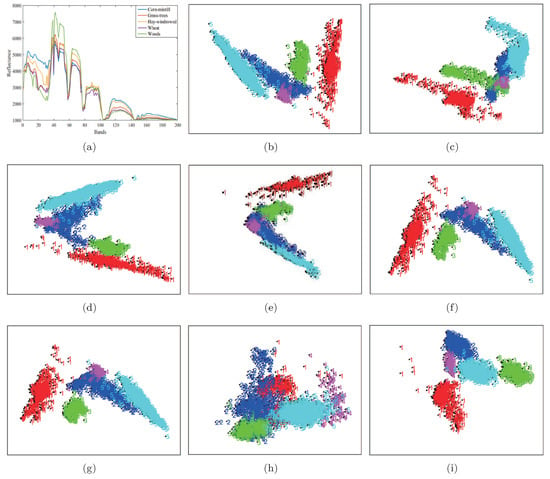
Figure 7.
Two-dimension embedding of different DR methods on the Indian Pines data set. (a) Spectral signatures; (b) PCA; (c) NPE; (d) LPP; (e) SDE; (f) LFDA; (g) MMC; (h) MFA; (i) LGSFA.
As shown in Figure 7, the results of PCA, NPE and LPP produced the scattered distribution of points from the same class and the overlapped points from different classes. This phenomenon may be caused by the unsupervised nature of the methods. The LFDA and MMC methods improved the compactness of points from the same class, while there still existed overlapping points between different classes. The reason is that LFDA and MMC originate from the theory of statistics that cannot effectively reveal the intrinsic manifold structure of data. SDE and MFA can reveal the intrinsic properties of data, but it may not effectively represent the manifold structure of hyperspectral data. This case resulted in some overlapping points between different classes. The proposed LGSFA method achieved better results than ohter DR methods, for the reason that LGSFA can effectively represent the manifold structure of hyperspectral data.
4.4. Experiments on the Salinas Data Set
To explore the classification accuracy with different numbers of intraclass neighbor points and interclass neighbor points, we randomly selected 60 samples from each class for training and the remaining samples for testing. After DR, the NN classifier was used to discriminate the test samples. Parameters k and were tuned with a set of and a set of , respectively. We repeated the experiment 10 times in each condition. In Figure 8, a curved surface map was depicted to display the average OAs with respect to parameters k and .
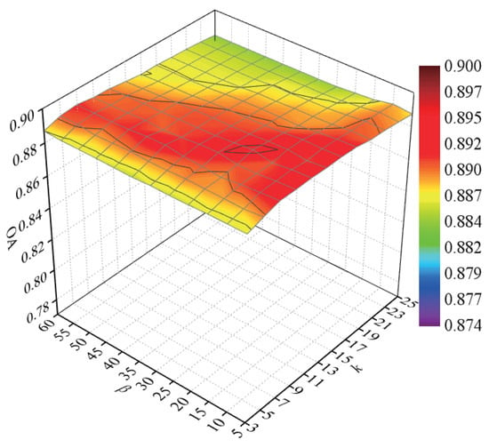
Figure 8.
OAs with respect to different numbers of neighbors on the Salinas data set.
According to Figure 8, with the increase in k, the OAs first increased and then decreased, for a small or large number of intraclass neighbor points cannot effectively represent the intrinsic structure of HSI. When the value of k was lower than 15, the OAs improved and then maintained a stable value with an increasing parameter . The OAs decreased quickly with a large value of when the value of k exceeded 15. The reason is that too large values of k and will result in the appearance of over-learning in the margins of interclass data. As a result, the parameters k and possesses a small influence on the classification accuracy for the Salinas data set, and we selected k and to 9 and 20 in the next experiments.
To analyze the influence of embedding dimension, we randomly selected 60 training samples for each class in Salinas data set and the NN classifier is used to discriminating the class of test samples. Figure 9 shows the average OAs under different dimensions with 10 times repeated experiment.
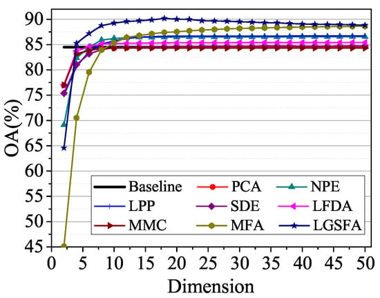
Figure 9.
OAs with respect to different dimensions on the Salinas data set.
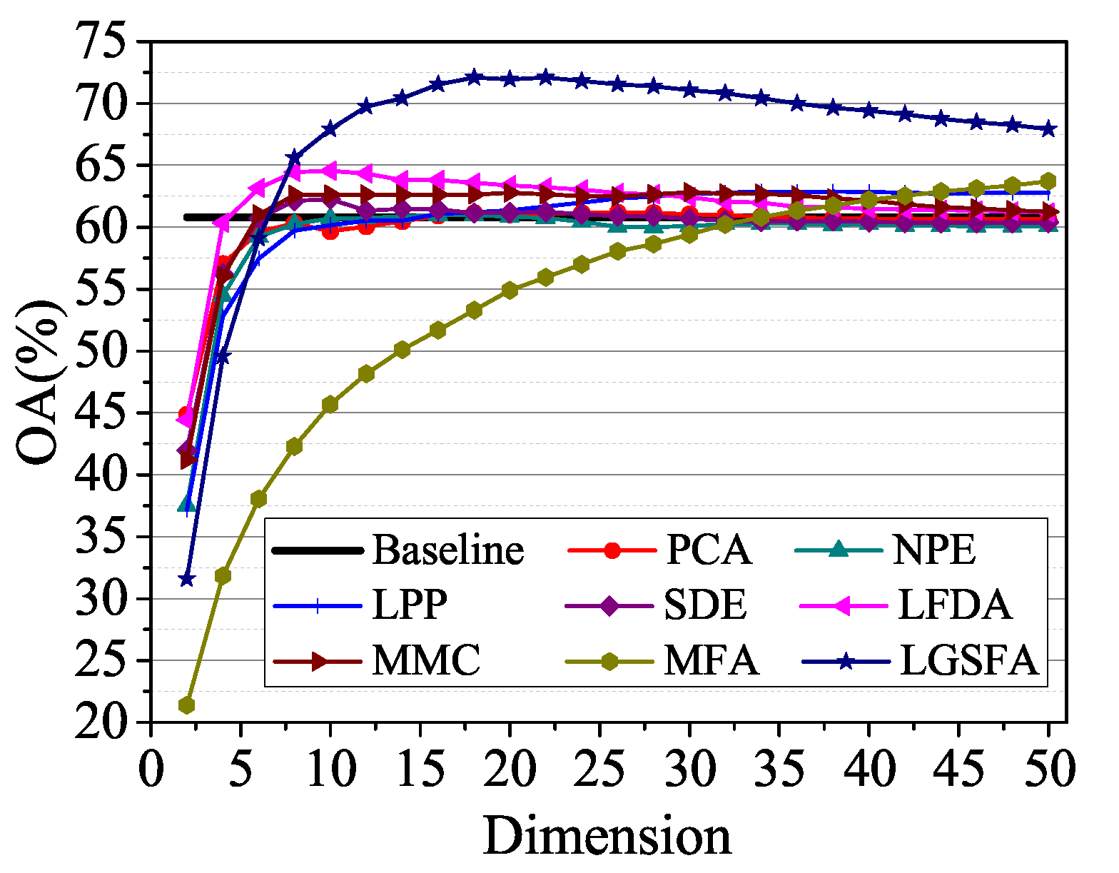
According to Figure 9, the classification accuracies improved with the increase of the embedding dimension and then reached a peak value. When the embedding dimension exceeded a certain value, the classification results of LGSFA began to decline, which resulted in the Hughes phenomena. NPE, LPP, LFDA, MFA, and LGSFA achieved better results than the baseline, thus indicating that the DR methods can reduce redundant information in HSI data. MFA and LGSFA generated higher OAs than other DR methods, the reason is that MFA and LGSFA can effectively reveal the intrinsic properties of hyperspectral data. In all the methods, LGSFA obtained the best classification accuracy, which indicates that LGSFA can better represent the intrinsic manifold of hyperspectral data that contains many homogenous areas.
To show the performance of LGSFA with different numbers of training samples, we randomly selected samples from each class for training and the remaining samples were used for testing. We adopted NN, SAM and SVMCK for the classification of test samples and repeated the experiment 10 times in each condition. The average OAs with STD and the average KCs are given in Table 1.

Table 1.
Classification results with different numbers of training samples on the Salinas data set (OA ± std (%) (KC)).
According to Table 1, the OAs and the KCs of each method improved as the increase of the number of training samples, because there is more priori information to represent the intrinsic properties of HSI. For different classifiers, each method with SVMCK possessed better classification accuracies than that with other classifiers, because SVMCK utilizes the spatial-spectral information that is beneficial to HSI classification. In all conditions, LGSFA achieved better results compared with MFA, and it also displayed the best accuracies than other DR methods. The reason is that LGSFA utilizes the neighbor points and corresponding intraclass reconstruction points to enhance the intraclass compactness and the interclass separability. It can effectively represent the intrinsic structure of HSI and obtain better discriminating features for classification.
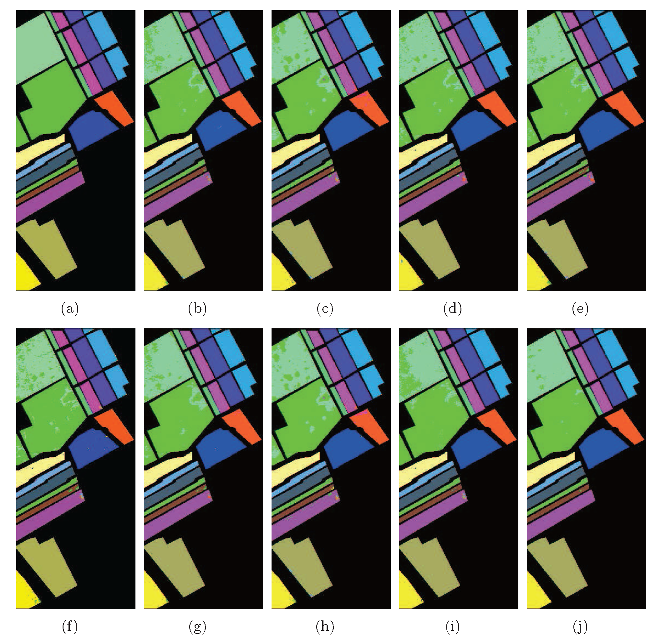
To explore the performance of LGSFA under different training conditions, we evaluated the classification accuracy of each class with a training set containing about 2% of samples per class. The remaining samples were used for testing. After the low-dimensional features were obtained with different DR methods, the SVMCK classifier was used to classify the test samples. The classification results are shown in Table 2 and corresponding classification maps are given in Figure 10.

Table 2.
Classification results of different DR methods with SVMCK on the Salinas data set.
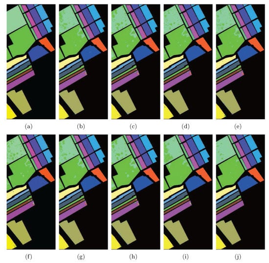
Figure 10.
Classification maps of different methods with SVMCK on the Salinas data set. (a) Ground truth; (b) Baseline (95.8%, 0.954); (c) PCA (94.8%, 0.942); (d) NPE (96.4%, 0.960); (e) LPP (96.0%, 0.955); (f) SDE (95.5%, 0.950); (g) LFDA (96.3%, 0.958); (h) MMC (94.7%, 0.941); (i) MFA (95.5%, 0.950); (j) LGSFA (99.2%, 0.991). Note that OA and KC are given in parentheses.
As shown in Table 2, the proposed method obtained the strongest classification effect in most classes and achieved the best OA, AA, and KC. LGSFA is clearly effective in revealing the intrinsic manifold structure of HSI, and it extracts better discriminating features for classification. The Baseline method cost more running time than other method for classification, because the hyperspectral data contains a large number of spectral bands to increase the computational cost of classification. LGSFA took more running time to reduce the dimensionality of data for the graph construction. However, LGSFA reduced the total running time for classification compared with the Baseline method, and it improved the classification performances compared with other methods.
According to Figure 10, LGSFA produced more homogenous areas than other DR methods, especially for the areas labeled as Grapes, Corn, Lettuce 4wk, Lettuce 7wk and Vinyard untrained.
4.5. Experiments on the Indian Pines Data Set
To analyze the performance of LGSFA with different land cover scenes, we utilized the AVIRIS Indian Pines data set for classification. In the experiment, we randomly selected samples from each class for training, and the remaining samples were used for testing. For the classes that are very small, i.e., Alfalfa, Grass/Pasture-mowed, and Oats, the number of training samples was set to if where is the number of the i-th class.
To explore the influence of parameters k and , 60 samples were randomly selected from each class for training, and the remaining samples were used for testing. The NN classifier was adopted to classify the test samples. Figure 11 shows the OAs with respect to parameters k and .

Figure 11.
OAs with respect to different numbers of neighbors on the Indian Pines data set.
According to Figure 11, the OAs improved quickly and then declined with the increase of k, because a small value of k cannot obtain enough information to reveal the intraclass structure and a large value of k will cause over-fitting to represent the intrinsic properties of hyperspectral data. The increased promoted the improvement of OAs, and then OAs reached to a stable peak value. To obtain optimal classification results, we set k and to 9 and 20 in the experiments.
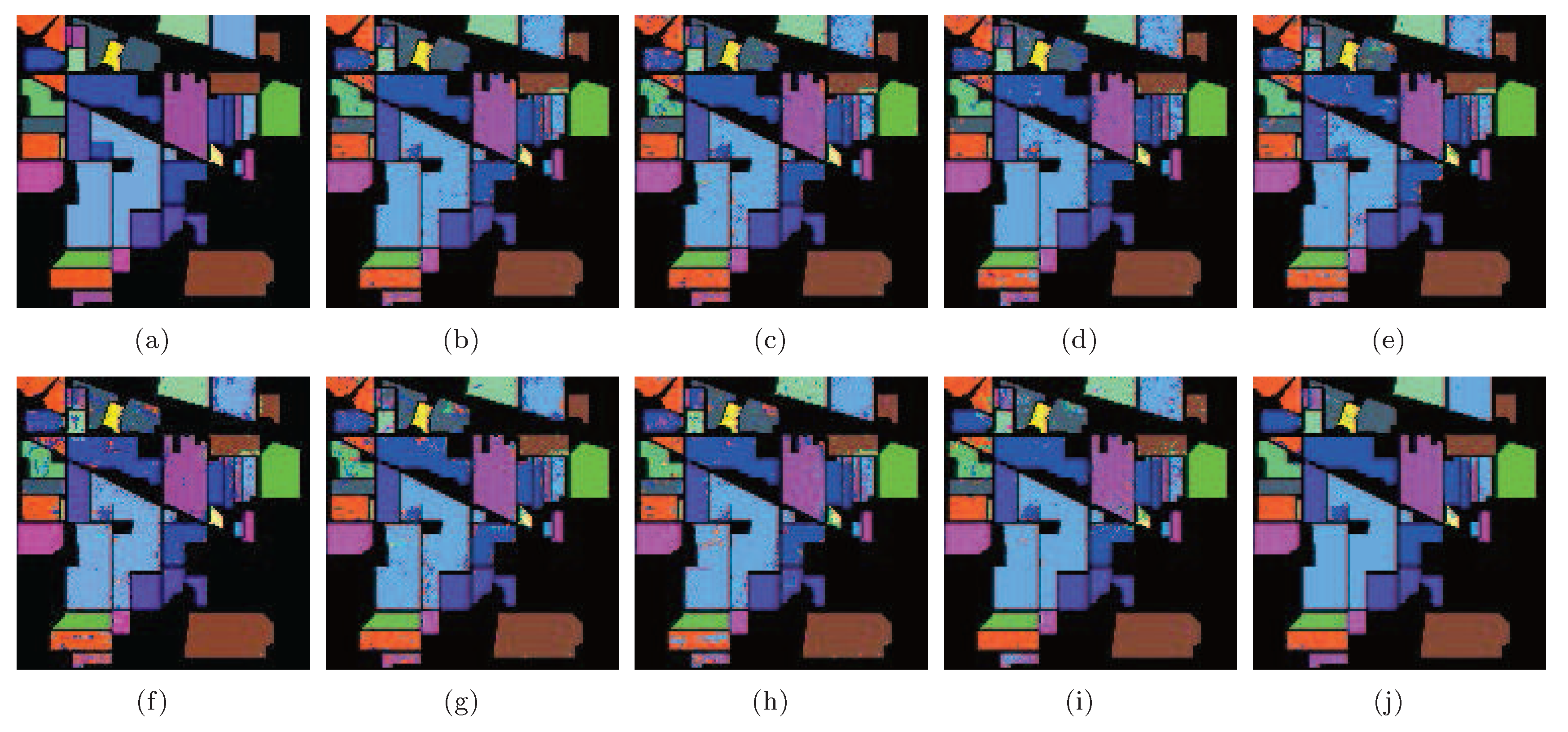
To analyze the classification accuracy under different embedding dimensions, 60 samples of each class were randomly selected as training set, and the NN classifier was used to classify the remaining samples. The results are shown in Figure 12. In the figure, LGSFA possessed the best classification accuracy, because it can better reveal the intrinsic manifold properties of hyperspectral data.
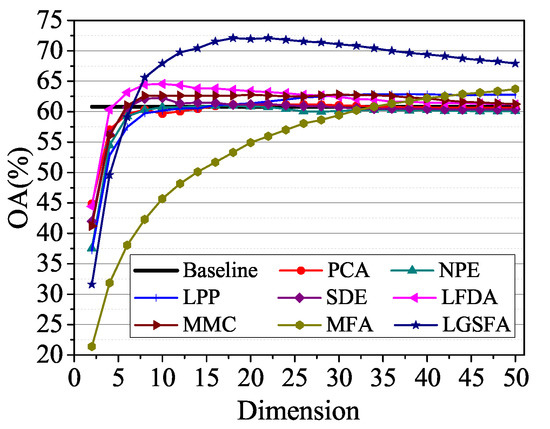
Figure 12.
OAs with respect to different dimensions on the Indian Pines data set.
To compare the results of each DR with different classifiers, we randomly selected 20, 40, 60, 80 samples from each class for training, and the remaining samples were used for testing. Each experiment was repeated 10 times and Table 3 shows the average OAs with STD and the average KCs.

Table 3.
Classification results with different numbers of training samples on the Indian Pines data set (OA ± std (%) (KC)).
As shown in Table 3, the classification accuracy of each DR method improved with the increasing number of training samples. The results of different DR methods with NN or SAM were unsatisfactory for the restricted discriminating power of NN or SAM. However, LGSFA with NN or SAM showed better results than other DR methods in most cases. The reason is that LGSFA effectively reveals the intrinsic manifold structure of hyperspectral data and obtains better discriminating features for classification. In addition, each DR method with SVMCK possessed better results than that with NN or SAM, and LGSFA with SVMCK achieved the best classification performances in all conditions.
To show the classification power of different methods for each class, 10% samples per class were selected for training, and other samples were used for testing. For very small classes, we take a minimum of ten training samples per class. The results of different methods with SVMCK are shown in Table 4.

Table 4.
Classification results of different DR methods with SVMCK on the Indian Pines data set.
According to Table 4, LGSFA achieved the best classification accuracy for most classes, as well as the best AA, OA, and KC among all the methods, because it can effectively represent the hidden manifold structure of hyperspectral data. The corresponding classification maps are displayed in Figure 13, which clearly indicates that the proposed method produces a smoother classification map compared with other methods in many areas.
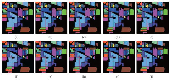
Figure 13.
Classification maps of different methods with SVMCK on the Indian Pines data set. (a) Ground truth; (b) Baseline (93.9%, 0.930); (c) PCA (91.8%, 0.907); (d) NPE (92.0%, 0.908); (e) LPP (91.0%, 0.897); (f) SDE (91.1%, 0.899); (g) LFDA (90.9%, 0.896); (h) MMC (89.9%, 0.885); (i) MFA (93.5%, 0.926); (j) LGSFA (98.1%, 0.978). Note that OA and KC are given in parentheses.
4.6. Experiments on the Urban Data Set
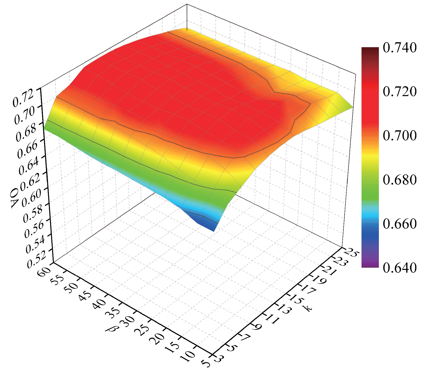
To further explore the effectiveness of LGSFA with different sensors, we selected the Urban data set captured by HYDICE sensor. We randomly selected 60 samples as training set to analyze OAs with respect to parameters k and . Figure 14 displays the classification results.
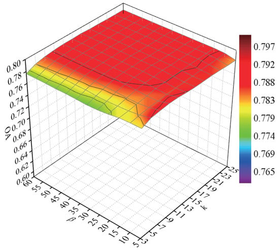
Figure 14.
OAs with respect to different numbers of neighbors on the Urban data set.
According to Figure 14, with the increase of intraclass neighbor k, the classification accuracies improved and then reached a stable value. The main reason is that the larger k will provide more effective information to reveal the intrinsic properties. The OAs also increased when the value of enlarged, because there is more information to represent the margin of different classes with a larger . To obtain better results, we set k and to 9 and 20 in the experiments.
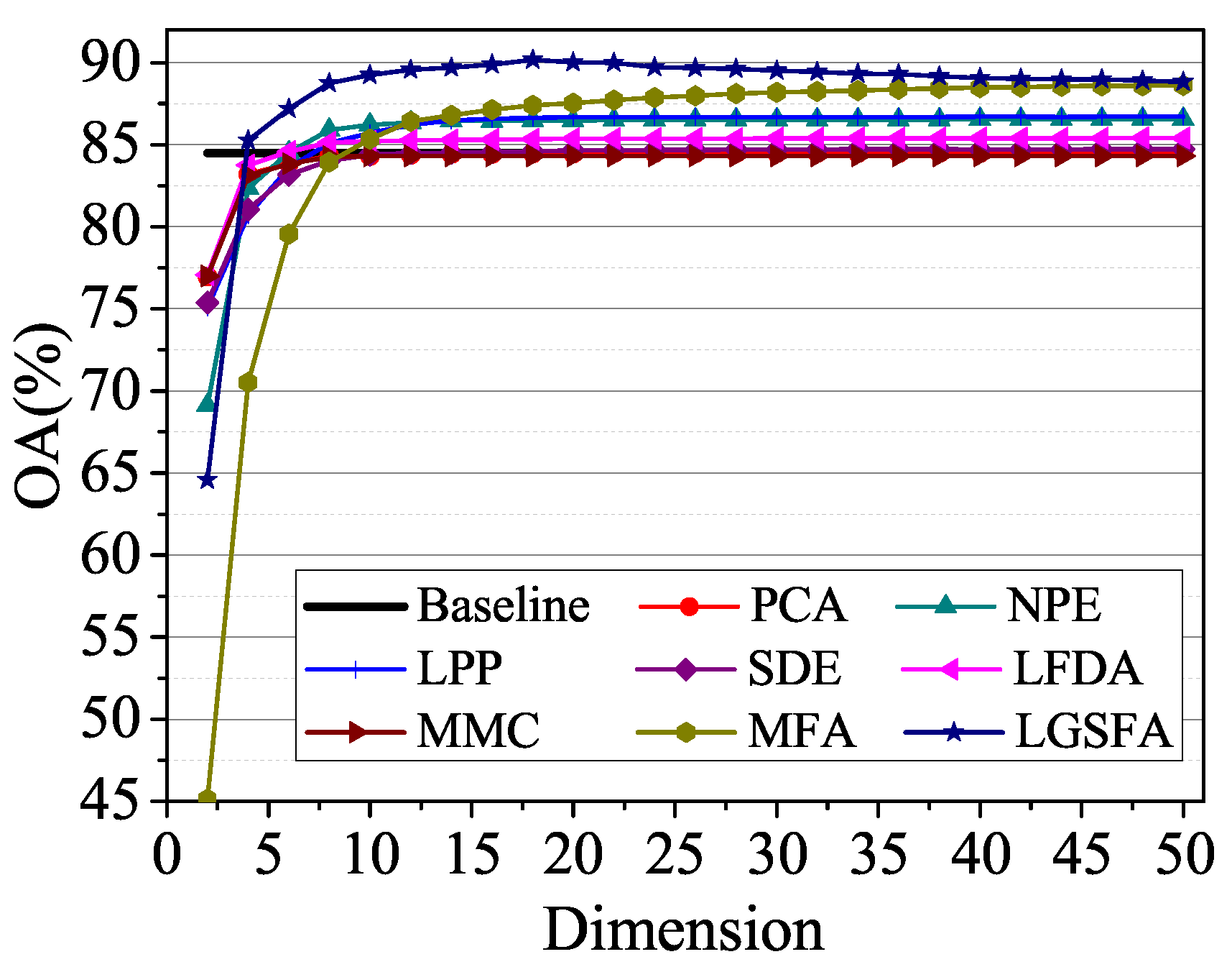
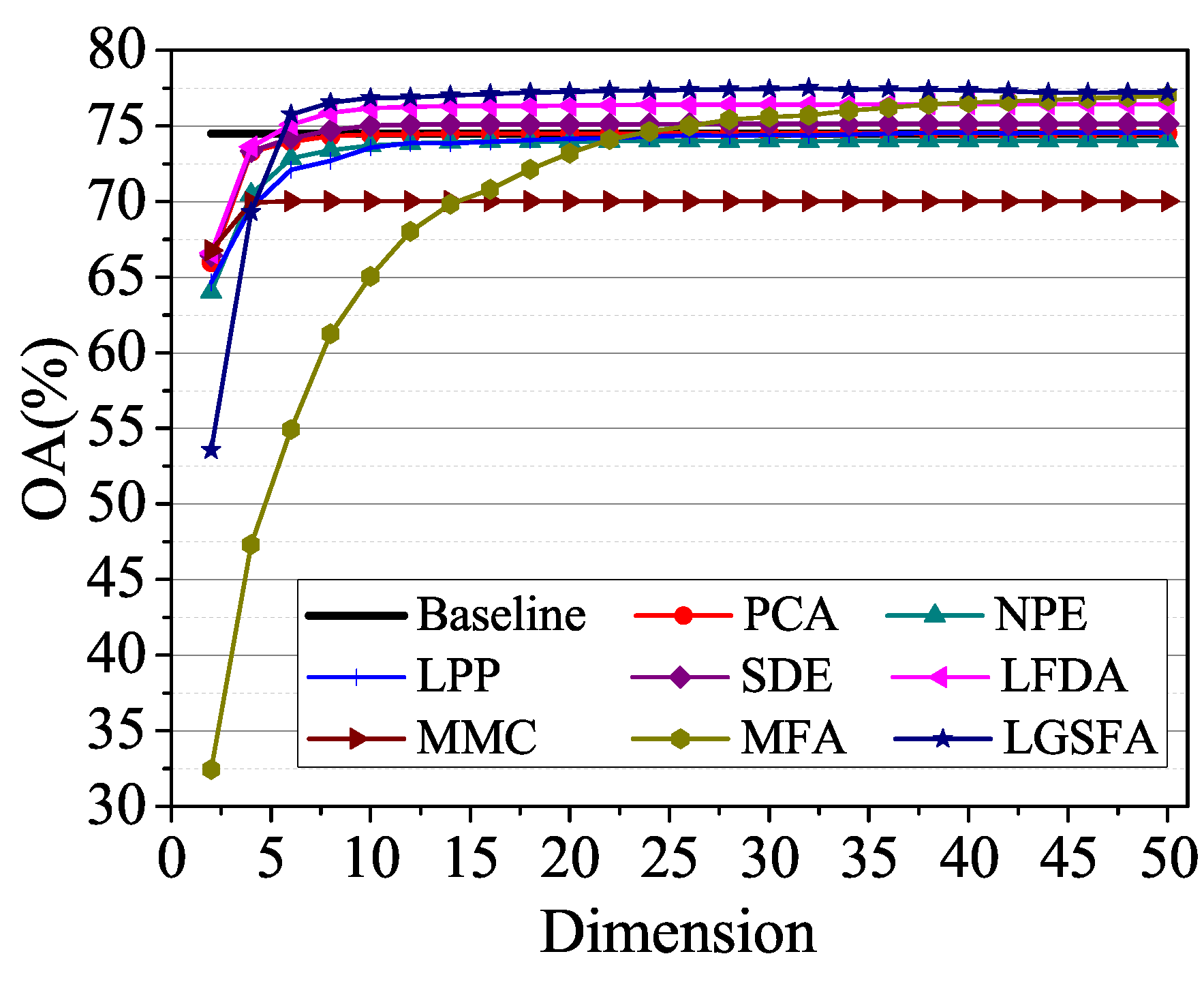
To explore the relationship between the classification accuracy and the embedding dimension, we randomly selected 60 samples form each class for training, and the remaining samples were used for testing. Figure 15 shows the OAs with different dimensions using the NN classifier. As shown in Figure 15, the OAs improved with the increase of the embedding dimension and then kept a balanced value. Compared with other methods, the proposed LGSFA method provided the best classification results.
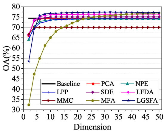
Figure 15.
OAs with respect to different dimensions on the Urban data set.
To compare the proposed method with other methods under different numbers of training samples, we randomly selected 20, 40, 60, 80 samples as training set, and the remaining samples were applied for testing. After DR with different methods, we adopted the NN, SAM, and SVMCK classifiers to discriminate the class of test samples with 10 times repeat experiments. The average OAs with std and KC (in parentheses) are given in Table 5.

Table 5.
Classification results with different numbers of training samples on the Urban data set (OA ± std (%) (KC)).
In Table 5, the results improved with the increase of the number of training samples in most conditions. Compared with other DR methods, LGSFA achieved the best OAs and KCs under different classifiers. Each DR method with SVMCK presented better classification results than other classifiers, and LGSFA with SVMCK possessed the best results in all cases. The experiment indicates that the proposed LGSFA method can effectively reveal the intrinsic manifold properties of hyperspectral data containing many homogenous areas.
To show the classification results of each class, we randomly selected 2% samples as training set, and the other samples were used for testing. The classification maps are shown in Figure 16.
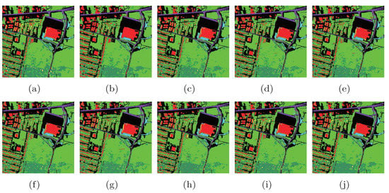
Figure 16.
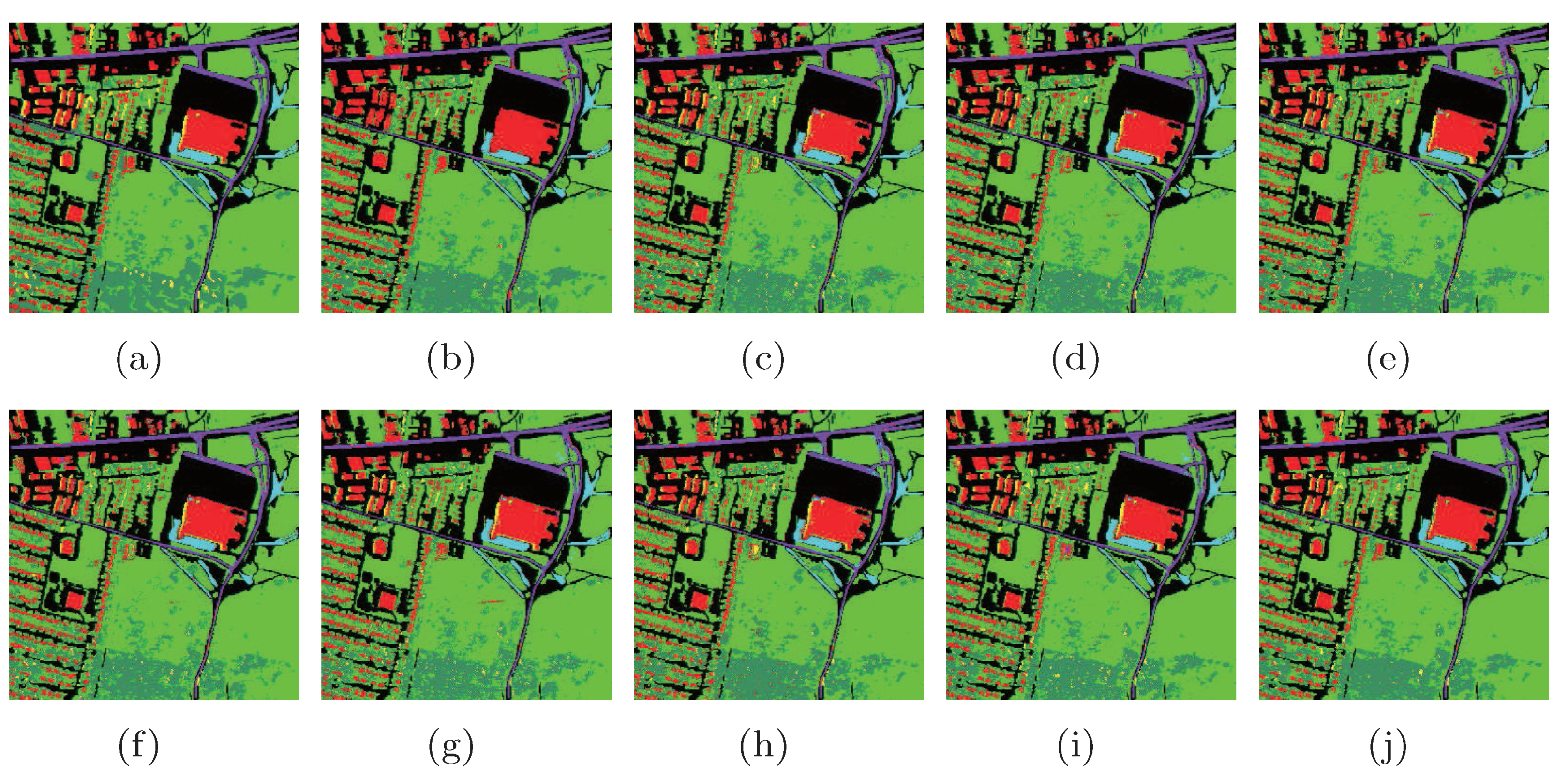
Classification maps of different methods with SVMCK on the Urban data set. (a) Ground truth; (b) Baseline (86.0%, 0.765); (c) PCA (85.1%, 0.750); (d) NPE (86.5%, 0.773); (e) LPP (87.0%, 0.781); (f) SDE (85.7%, 0.758); (g) LFDA (85.6%, 0.759); (h) MMC (86.1%, 0.765); (i) MFA (87.5%, 0.788); (j) LGSFA (88.8%, 0.809). Note that OA and KC are given in parentheses.
As shown in Figure 16, the LGSFA method displayed more similar compared with the ground truth. The corresponding numerical results are shown in Table 6. In the table, the proposed method obtained better classification accuracy in most classes and achieved the best AA, OA, and KC among all the methods, which indicates that LGSFA is more beneficial to represent the hidden information of hyperspectral data.

Table 6.
Classification results of different DR methods with SVMCK on the Urban data set.
4.7. Discussion
The following interesting points are revealed in the experiments on the Salinas, Indian Pines, and Urban HSI data sets.
- The proposed LGSFA method consistently outperforms Baseline, PCA, NPE, LPP, SDE, LFDA, MMC and MFA in most conditions on three real HSI data sets. The reason for this appearance is that LGSFA utilizes neighbor points and corresponding intraclass reconstruction points to construct the intrinsic and penalty graphs, while MFA just uses the neighbor points to construct the intrinsic and penalty graphs. That is to say, our proposed method can effictively compact the intraclass data and separate the interclass data, and it can capture more intrinsic information hidden in HSI data sets than other methods.
- It is clear that LGSFA produces a smoother classification map and achieves better accuracy compared with other methods in most classes. LGSFA effectively reveal the intrinsic manifold structures of hyperspectral data. Thus, this method obtains good discriminating features and improves the classification performance of the NN, SAM and SVMCK classifiers for hyperspectral data.
- In the experiments, it is noticeable that the SVMCK classifier always performs better than NN and SAM. The reason is that SVMCK applies the spatial and spectral information while NN and SAM only use the spectral information for HSI classification.
- With the running time of different DR methods, the computational complexity of LGSFA depends on the number of bands, training samples, and neighbor points. The proposed method costs more time than other DR algorithms. The reason is that LGSFA needs much running time to construct the intrinsic graph and the penalty graph.
- In the experiments of two-dimension embedding, LGSFA achieves better distribution for data points than other DR methods. The results show that LGSFA can improve the intra-manifold compactness and the inter-manifold separability to enhance the diversity of data from different classes.
5. Conclusions
In this paper, we proposed a new method called LGSFA for DR of HSI. The proposed LGSFA method constructs an intrinsic graph and a penalty graph using the intraclass neighbor points, the interclass neighbor points and their corresponding reconstruction points. It utilizes neighbor points and corresponding intraclass reconstruction points to improve the intraclass compactness and the interclass separability. As a result, LGSFA effectively reveals the intrinsic manifold structure of hyperspectral data to extract effective discriminating features for classification. Experiments on the Salinas, Indian Pines, and Urban data sets show that the proposed method achieves better results than other state-of-the-art methods in most conditions and LGSFA with SVMCK obtains the best classification accuracy. Our future work will focus on how to improve the computational efficiency and the misclassified pixels.
Acknowledgments
The authors would like to thank David A Landgrebe at Purdue University for providing the AVIRIS Indian Pines data set, and Lee F Johnson and J Anthony Gualtieri for providing the AVIRIS Salinas data set. The authors would like to thank the anonymous reviewers and associate editor for their valuable comments and suggestions to improve the quality of the paper. This work was supported in part by the National Science Foundation of China under Grant 41371338, the Visiting Scholar Foundation of Key Laboratory of Optoelectronic Technology and Systems (Chongqing University), Ministry of Education, and China Postdoctoral Program for Innovative Talent under Grant BX201700182.
Author Contributions
Fulin Luo was primarily responsible for mathematical modeling and experimental design. Hong Huang contributed to the experimental analysis and revised the paper. Yule Duan completed the comparison with other methods. Jiamin Liu provided important suggestions for improving the paper. Yinghua Liao provided some suggestions in the revised manuscript.
Conflicts of Interest
The authors declare no conflict of interest.
References
- Liang, H.M.; Li, Q. Hyperspectral imagery classification using sparse representations of convolutional neural network features. Remote Sens. 2016, 8, 919. [Google Scholar] [CrossRef]
- He, W.; Zhang, H.Y.; Zhang, L.P.; Philips, W.; Liao, W.Z. Weighted sparse graph based dimensionality reduction for hyperspectral images. IEEE Geosci. Remote Sens. Lett. 2016, 13, 686–690. [Google Scholar] [CrossRef]
- Zhong, Y.F.; Wang, X.Y.; Zhao, L.; Feng, R.Y.; Zhang, L.P.; Xu, Y.Y. Blind spectral unmixing based on sparse component analysis for hyperspectral remote sensing imagery. J. Photogramm. Remote Sens. 2016, 119, 49–63. [Google Scholar] [CrossRef]
- Zhou, Y.C.; Peng, J.T.; Chen, C.L.P. Dimension reduction using spatial and spectral regularized local discriminant embedding for hyperspectral image classification. IEEE Trans. Geosci. Remote Sens. 2015, 53, 1082–1095. [Google Scholar] [CrossRef]
- Feng, F.B.; Li, W.; Du, Q.; Zhang, B. Dimensionality reduction of hyperspectral image with graph-based discriminant analysis considering spectral similarity. Remote Sens. 2017, 9, 323. [Google Scholar] [CrossRef]
- Sun, W.W.; Halevy, A.; Benedetto, J.J.; Czaja, W.; Liu, C.; Wu, H.B.; Shi, B.Q.; Li, W.Y. Ulisomap based nonlinear dimensionality reduction for hyperspectral imagery classification. J. Photogramm. Remote Sens. 2014, 89, 25–36. [Google Scholar] [CrossRef]
- Rathore, M.M.U.; Paul, A.; Ahmad, A.; Chen, B.W.; Huang, B.; Ji, W. Real-time big data analytical architecture for remote sensing application. IEEE J. Sel. Top. Appl. Earth Obs. Remote Sens. 2015, 8, 4610–4621. [Google Scholar] [CrossRef]
- Tong, Q.X.; Xue, Y.Q.; Zhang, L.F. progress in hyperspectral remote sensing science and technology in China over the past three decades. IEEE J. Sel. Top. Appl. Earth Obs. Remote Sens. 2014, 7, 70–91. [Google Scholar] [CrossRef]
- Huang, H.; Luo, F.L.; Liu, J.M.; Yang, Y.Q. Dimensionality reduction of hyperspectral images based on sparse discriminant manifold embedding. J. Photogramm. Remote Sens. 2015, 106, 42–54. [Google Scholar] [CrossRef]
- Zhang, L.P.; Zhong, Y.F.; Huang, B.; Gong, J.Y.; Li, P.X. Dimensionality reduction based on clonal selection for hyperspectral imagery. IEEE Trans. Geosci. Remote Sens. 2007, 45, 4172–4186. [Google Scholar] [CrossRef]
- Cheng, G.L.; Zhu, F.Y.; Xiang, S.M.; Wang, Y.; Pan, C.H. Semisupervised hyperspectral image classification via discriminant analysis and robust regression. IEEE J. Sel. Top. Appl. Earth Obs. Remote Sens. 2016, 9, 595–608. [Google Scholar] [CrossRef]
- Shi, Q.; Zhang, L.P.; Du, B. Semisupervised discriminative locally enhanced alignment for hyperspectral image classification. IEEE Trans. Geosci. Remote Sens. 2013, 51, 4800–4815. [Google Scholar] [CrossRef]
- Huang, H.; Yang, M. Dimensionality reduction of hyperspectral images with sparse discriminant embedding. IEEE Trans. Geosci. Remote Sens. 2015, 53, 5160–5169. [Google Scholar] [CrossRef]
- Yang, S.Y.; Jin, P.L.; Li, B.; Yang, L.X.; Xu, W.H.; Jiao, L.C. Semisupervised dual-geometric subspace projection for dimensionality reduction of hyperspectral image data. IEEE Trans. Geosci. Remote Sens. 2014, 52, 3587–3593. [Google Scholar] [CrossRef]
- Zhang, L.F.; Zhang, L.P.; Tao, D.C.; Huang, X.; Du, B. Compression of hyperspectral remote sensing images by tensor approach. Neurocomputing 2015, 147, 358–363. [Google Scholar] [CrossRef]
- Cheng, X.M.; Chen, Y.R.; Tao, Y.; Wang, C.Y.; Kim, M.S.; Lefcourt, A.M. A novel integrated PCA and FLD method on hyperspectral image feature extraction for cucumber chilling damage inspection. Trans. ASAE 2004, 47, 1313–1320. [Google Scholar] [CrossRef]
- Guan, L.X.; Xie, W.X.; Pei, J.H. Segmented minimum noise fraction transformation for efficient feature extraction of hyperspectral images. Pattern Recognit. 2015, 48, 3216–3226. [Google Scholar]
- Cai, D.; He, X.; Han, J. Semi-supervised discriminant analysis. In Proceedings of the International Conference on Computer Vision, Rio de Janeiro, Brazil, 14–21 October 2007; pp. 1–7. [Google Scholar]
- Li, H.F.; Jiang, T.; Zhang, K.S. Efficient and robust feature extraction by maximum margin criterion. IEEE Trans. Neural Netw. 2006, 17, 157–165. [Google Scholar] [CrossRef] [PubMed]
- Sugiyama, M. Dimensionality reduction of multimodal labeled data by local Fisher discriminant analysis. J. Mach. Learn. Res. 2007, 8, 1027–1061. [Google Scholar]
- Shao, Z.; Zhang, L. Sparse dimensionality reduction of hyperspectral image based on semi-supervised local Fisher discriminant analysis. Int. J. Appl. Earth Obs. Geoinf. 2014, 31, 122–129. [Google Scholar] [CrossRef]
- Bachmann, C.M.; Ainsworth, T.L.; Fusina, R.A. Exploiting manifold geometry in hyperspectral imagery. IEEE Trans. Geosci. Remote Sens. 2005, 43, 441–454. [Google Scholar] [CrossRef]
- Yang, H.L.; Crawford, M.M. Domain adaptation with preservation of manifold geometry for hyperspectral image classification. IEEE J. Sel. Top. Appl. Earth Obs. Remote Sens. 2016, 9, 543–555. [Google Scholar] [CrossRef]
- Ma, L.; Zhang, X.F.; Yu, X.; Luo, D.P. Spatial regularized local manifold learning for classification of hyperspectral images. IEEE J. Sel. Top. Appl. Earth Obs. Remote Sens. 2016, 9, 609–624. [Google Scholar] [CrossRef]
- Tang, Y.Y.; Yuan, H.L.; Li, L.Q. Manifold-Based Sparse Representation for Hyperspectral Image Classification. IEEE Trans. Geosci. Remote Sens. 2014, 52, 7606–7618. [Google Scholar] [CrossRef]
- Zhang, L.F.; Zhang, Q.; Zhang, L.P.; Tao, D.C.; Huang, X.; Du, B. Ensemble manifold regularized sparse low-rank approximation for multiview feature embedding. Pattern Recognit. 2015, 48, 3102–3112. [Google Scholar] [CrossRef]
- Tenenbaum, J.B.; de Silva, V.; Langford, J.C. A global geometric framework for nonlinear dimensionality reduction. Science 2000, 290, 2319–2323. [Google Scholar] [CrossRef] [PubMed]
- Belkin, M.; Niyogi, P. Laplacian eigenmaps for dimensionality reduction and data representation. Neural Comput. 2003, 15, 1373–1396. [Google Scholar] [CrossRef]
- Roweis, S.T.; Saul, L.K. Nonlinear dimensionality reduction by locally linear embedding. Science 2000, 290, 2323–2326. [Google Scholar] [CrossRef] [PubMed]
- Wang, Z.Y.; He, B.B. Locality perserving projections algorithm for hyperspectral image dimensionality reduction. In Proceedings of the 19th International Conference on Geoinformatics, Shanghai, China, 24–26 June 2011; pp. 1–4. [Google Scholar]
- He, X.F.; Cai, D.; Yan, S.C.; Zhang, H.J. Neighborhood preserving embedding. In Proceedings of the 10th International Conference on Computer Vision, Beijing, China, 17–21 October 2005; pp. 1208–1213. [Google Scholar]
- Yan, S.C.; Xu, D.; Zhang, B.Y.; Zhang, H.J.; Yang, Q.; Lin, S. Graph embedding and extensions: A general framework for dimensionality reduction. IEEE Trans. Pattern Anal. Mach. Intell. 2007, 29, 40–51. [Google Scholar] [CrossRef] [PubMed]
- Chen, Y.S.; Zhao, X.; Jia, X.P. Spectral-spatial classification of hyperspectral data based on deep belief network. IEEE J. Sel. Top. Appl. Earth Obs. Remote Sens. 2015, 8, 2381–2392. [Google Scholar] [CrossRef]
- Feng, Z.X.; Yang, S.Y.; Wang, S.G.; Jiao, L.C. Discriminative spectral-spatial margin-based semisupervised dimensionality reduction of hyperspectral data. IEEE Geosci. Remote Sens. Lett. 2015, 12, 224–228. [Google Scholar] [CrossRef]
- Luo, F.L.; Huang, H.; Ma, Z.Z.; Liu, J.M. Semisupervised sparse manifold discriminative analysis for feature extraction of hyperspectral images. IEEE Trans. Geosci. Remote Sens. 2016, 54, 6197–6211. [Google Scholar] [CrossRef]
- Camps-Valls, G.; Gomez-Chova, L.; Munoz-Mari, J.; Vila-Frances, J.; Calpe-Maravilla, J. Composite kernels for hyperspectral image classification. IEEE Geosci. Remote Sens. Lett. 2006, 3, 93–97. [Google Scholar] [CrossRef]
- Chang, C.C.; Lin, C.J. LIBSVM: A Library for Support Vector Machines. 2001. Available online: http://www.csie.ntu.edu.tw/~cjlin/libsvm (accessed on 18 May 2017).
© 2017 by the authors. Licensee MDPI, Basel, Switzerland. This article is an open access article distributed under the terms and conditions of the Creative Commons Attribution (CC BY) license (http://creativecommons.org/licenses/by/4.0/).

