1. Introduction
Alongside the rapid development of remote sensing platforms and sensors, the volume of remotely sensed imagery has also tremendously increased. Because of the large data volumes, the exploration and information mining from remote sensing archives is becoming increasingly difficult. Content-based image retrieval (CBIR) is one of the most active research areas in computer vision. CBIR is also widely used in remote sensing image retrieval, as it does not require the presence of semantic tags, which are rarely available and expensive to assign. In order to improve the situation of the low degree of utilization of the existing large archives of remotely sensed imagery, many studies [
1,
2,
3,
4,
5,
6] have addressed the application of CBIR to remotely sensed imagery. Li et al. [
7] proposed a remote sensing image retrieval approach by adopting convolutional neural networks to extract unsupervised features. Demir and Bruzzone [
8,
9] introduced the hashing methods for large-scale remote sensing (RS) retrieval problems to provide highly time-efficient and accurate search capability within huge data archives. Aptoula [
10,
11] applied global morphological texture descriptors to the problem of content-based remote sensing image retrieval. Local description strategies and visual vocabularies were widely adopted by remote sensing content-based retrieval and scene classification [
12,
13,
14,
15,
16,
17,
18,
19,
20]. To better manage remotely sensed data, Alonso et al. [
21,
22] designed a system and tools for effectively querying and understanding the available data archives. To improve Earth observation (EO) image retrieval results, Research projects like EOLib [
23] and TELEIOS [
24] have introduced the use of EO image metadata and linked data as query parameters. Along with EO image analysis data, an information layer extracted from OpenStreetMaps was used in the learning stage of the retrieval system [
25]. There are also systems for the retrieval and analysis of remote sensing images time series, such as knowledge-driven information mining (KIM) [
2], image information mining in time series (IIM-TS) [
26], and the PicSOM system based on self-organizing maps (SOM) [
27]. We should note that with the rapid growth of imagery databases, the number of image-derived products such as land use/land cover (LULC) products derived from high spatial resolution satellite or aerial images has also increased. These derived products allow us to retrieve remotely-sensed scenes with a higher efficiency and accuracy, when compared to retrieval based directly on imagery. Recently, a CBIR-like system specifically designed for category valued geospatial databases in general and for LULC databases in particular was proposed in [
28]. The authors designed a pattern signature using only two features: the distribution of the labels and the size of the patches (which refer to the connected regions of the same label) [
29]. Furthermore, a scene pattern signature was computed, which is the probability distribution of a 2-D variable with respect to the label and patch size. Based on the approach proposed in [
28], LandEx (Landscape Explorer)—a content-based map retrieval (CBMR) system—was designed [
30]. LandEx shares almost the same characteristics as the CBIR systems. In some cases, the distribution of the labels is enough for the retrieval task. However, for more complicated scenes with specific spatial patterns of different labels, the spatial relationships also need to be taken into consideration.
In this letter, we propose a CBIR-like remotely sensed scene retrieval system for use with LULC databases. To consider the spatial relationships of the labels in a scene, we propose a scene signature extraction method motivated by the grey level co-occurrence matrix (GLCM), which is utilized to compute the texture feature of the image. The similarity measurement we adopt is the cosine similarity, which is appropriate for our requirements even though it is simple. The scene signature can describe not only the probability distribution of the labels, but also the spatial relations. The CBMR system could also benefit from this approach.
In this study, we built a base signature library for the National Land Cover Database (NLCD) for 2006 [
31,
32]. The library consisted of the signature of every base block (
pixels). By using the label co-occurrence matrix (LCM), the similarity between scenes of various sizes can be computed. In contrast, in most of the traditional retrieval systems, only the similarity between scenes of the same size can be computed. More specifically, signatures of the scenes with larger sizes (e.g.,
,
, etc.) can be rapidly computed from the signature library, instead of re-computing the signatures for the whole database. In addition, the output of the retrieval results is more flexible. In addition to the similarity map measured between the reference scene and the whole database, we can also output the best-matching scene tiles, with the sizes not limited to the size of the analysis window.
The rest of this letter is organized as follows.
Section 2 briefly describes the proposed scene retrieval approach and introduces the proposed CBMR system in detail. In
Section 3, we describe the series of experiments carried out to compare the scene retrieval performance of the proposed method with that of previous methods. A summary is provided in
Section 4, along with a discussion of the achieved results.
2. Methodology
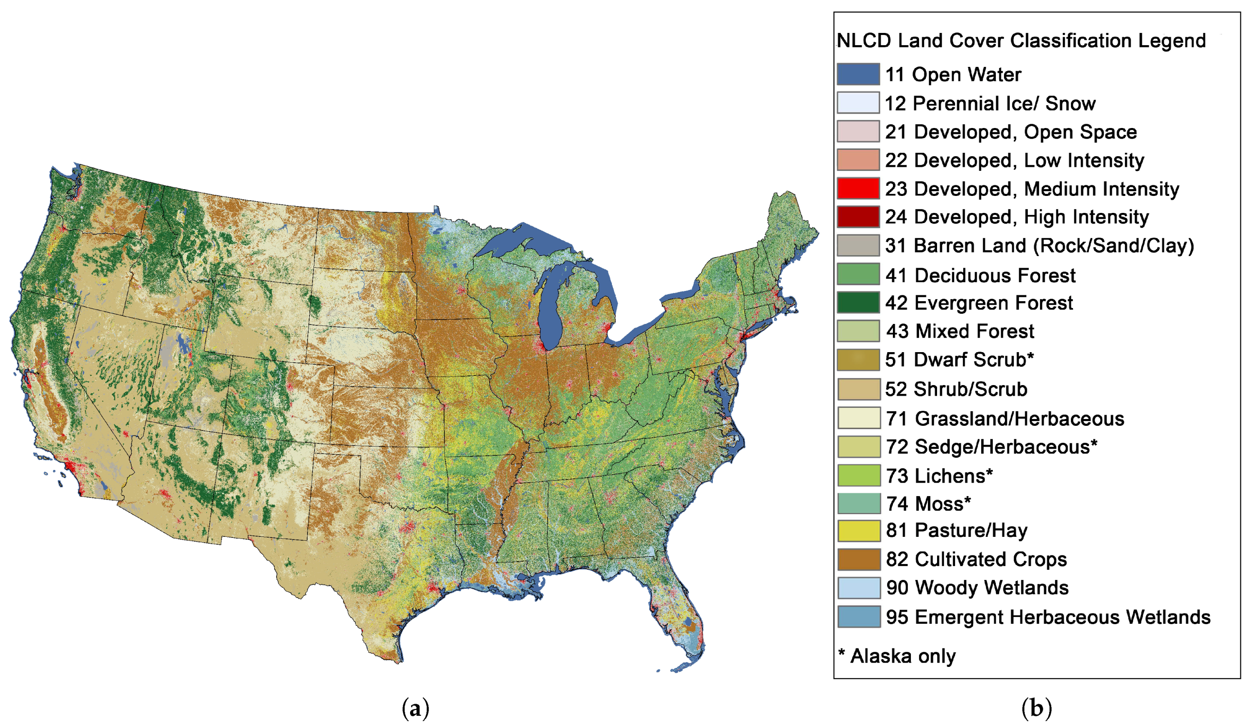
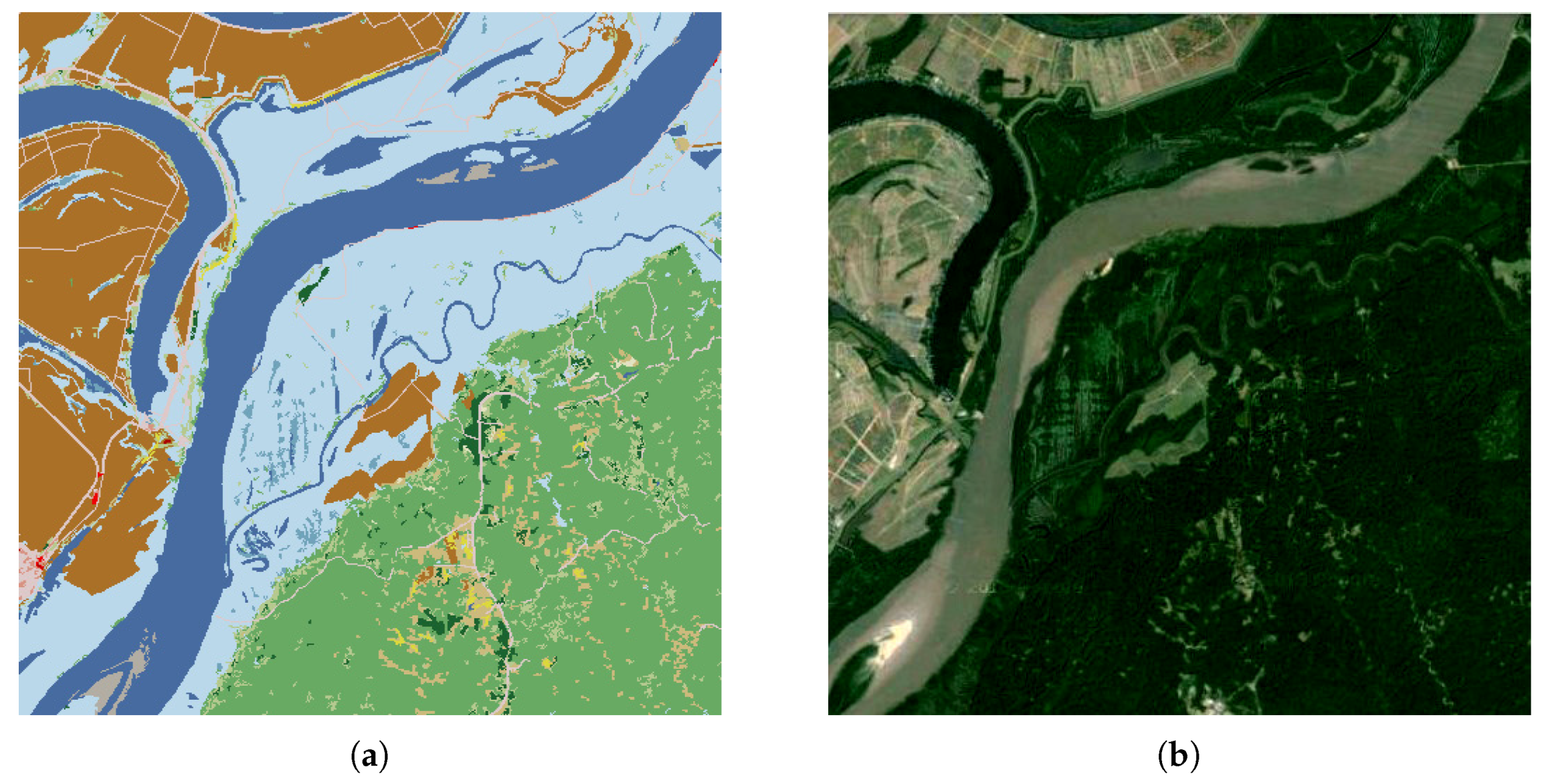
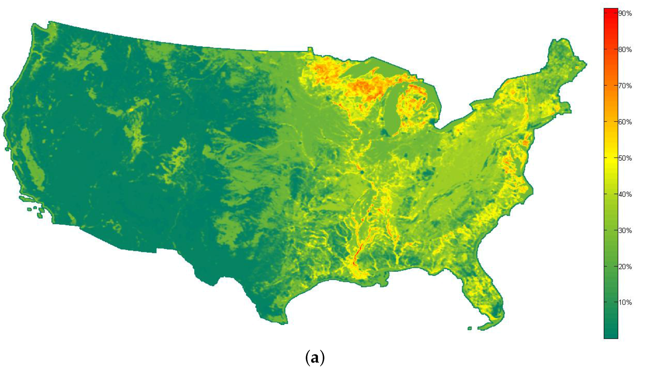
This section provides a summary of the proposed approach for the retrieval of alike land-cover scenes from the NLCD 2006 database [
31,
32] (see
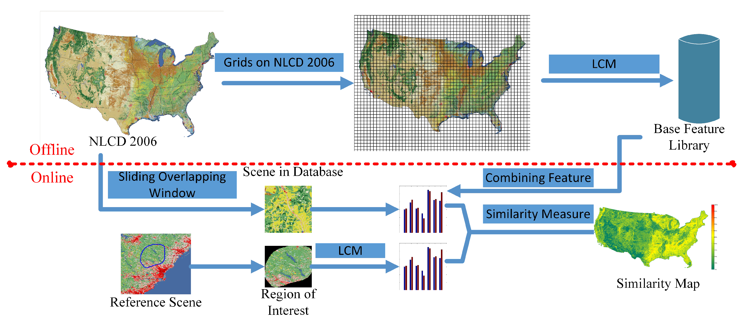
Figure 1), which is shown by a flow chart in
Figure 2. NLCD 2006 is a 16-class land cover classification product that covers the United States at a spatial resolution of 30 m.
The process can be divided into two main parts: (1) the off-line building of the signature library from the original LULC database; and (2) computation of the similarity between the selected reference scene and the scenes in the database with a given size (width, height, and offset). Constructing the signature library is the foundation of the retrieval system.
2.1. Label Co-Occurrence Matrix
The scene signature that we propose is inspired by the grey level co-occurrence matrix (GLCM) [
35], and is utilized to extract the texture feature of the image. The principle of the GLCM has also been used in other applications and data. Barnsley et al. [
36] designed a kernel-based procedure referred to as SPARK (spatial reclassification kernel) to examine both the frequency and the spatial arrangement of the class (land-cover) labels within a square kernel. To improve the classification of buildings, Zhang et al. [
37] adopted modified co-occurrence matrix-based filtering. In the method proposed in [
38], pairs of neighboring cells are regarded as primitive features. The primitive features are then extracted and counted to form a histogram to represent the pattern of a tile. The GLCM has also been used to describe landscape structure [
39]. In this letter, based on the same idea, we propose the label co-occurrence matrix for a LULC scene, which is defined as:
where
represents the number of elements contained in set
A, and
i and
j correspond to the labels of pixel
and
in the scene. For a scene I, the co-occurrence matrices are computed at four orientations:
where
d is the distance parameter, which we set to 1. It can be seen that the LCM contains not only the first-order statistics of the labels in a scene (e.g., the histogram), but also the second-order statistics (i.e., the spatial relationships between adjacent pixels). In order to have a (relatively) rotation-invariant feature (because orientation information is not important in remote sensing), we sum the four co-occurrence matrices. For a scene
I, its LCM should then be:
where
n is the amount of labels of the given scene, and
H is a symmetrical matrix of which the dimension is
n. Due to the symmetry of
H we can only use matrix elements of the lower triangle to form a vector
V (the dimension of
V is
).
Then, a final vector F which we can have after a normalization process for V is used as the descriptor for the scene.
where
.
2.2. Similarity Measure
A number of different similarity measurements, including the Manhattan distance, the Hausdorff distance, the Mahalanobis distance, Kullback–Leibler divergence [
40], Jeffrey divergence [
41], etc., have been proposed for CBIR. In this letter, we chose cosine similarity for the similarity measure to be always within the range of 0 to 1 due to the elements in the signature vectors being positive. The scenes are described by a signature vector computed by the LCM. Given two scenes
k and
l, their corresponding signature vectors are
and
, computed using Equation (
9). The similarity between the two scenes is defined as:
2.3. Determining the Signature of the Candidate Scene by Combining the Signatures in the Base Signature Library
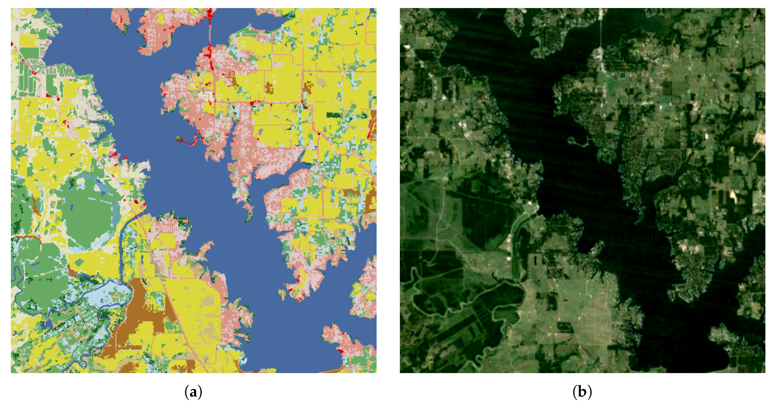
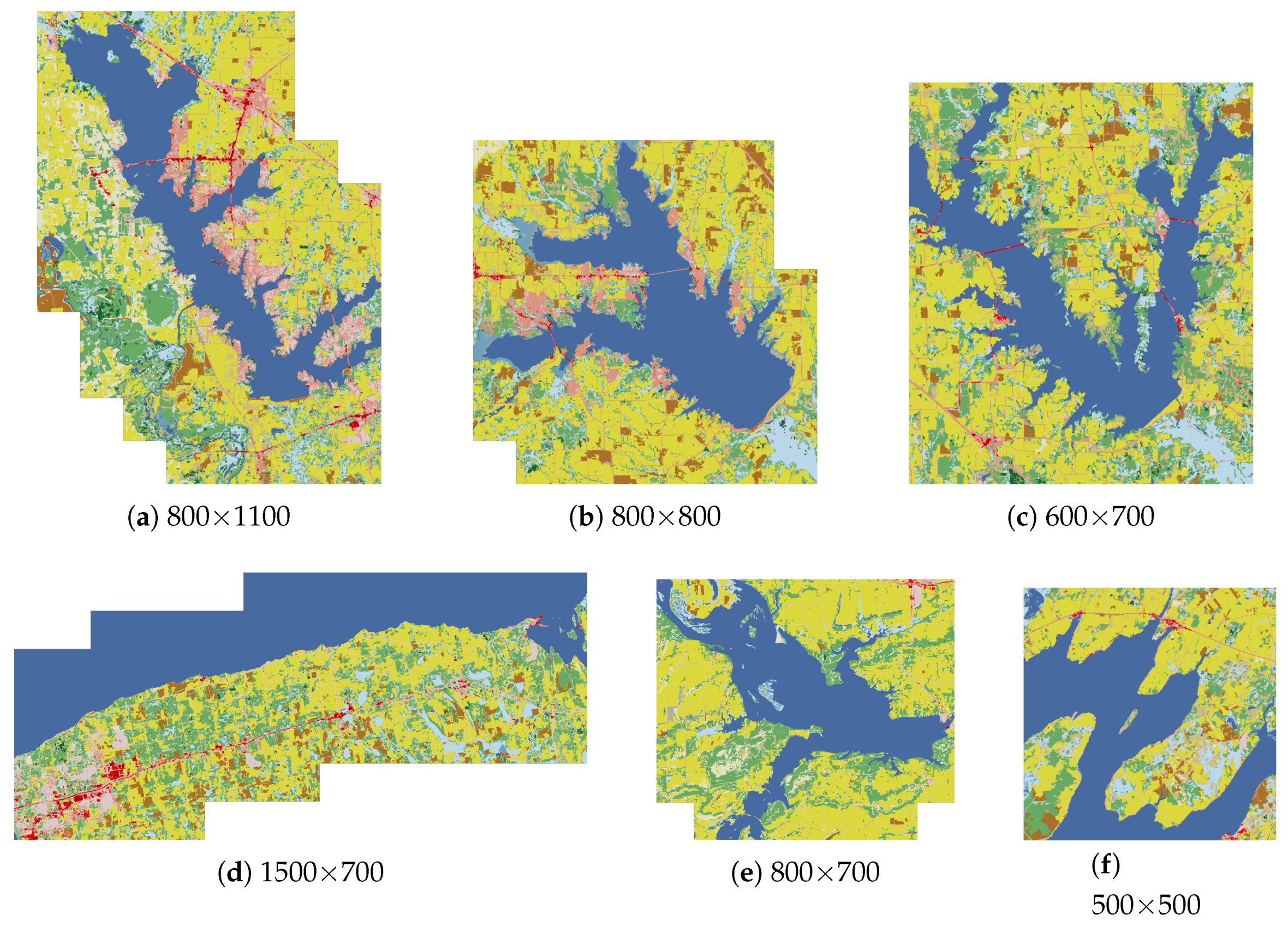
In contrast to the traditional retrieval systems (for which the reference scene can only be of fixed size), we enable the user to select the reference scene more flexibly (see
Figure 3b). The sizes of the retrieved scenes can also be varied according to the requirement of the user during each retrieval.
The ability to return scenes with varied sizes relies on the computation of the scene signature. The construction process will be explained below in detail. Given that the database is a land cover scene in size, with width and height both 100 pixels. We first divided the whole map into small patches of
grids without overlap. The LCM was then computed for each patch, and was stored as the base signature library. Suppose that a ROI of
pixels is selected as the reference scene, and the user wants to obtain scenes of the same size with similar content. We first compute the LCM for the selected reference scene. For the signatures of the scenes in the database, we combine the adjacent
base signatures in the library as the signature of the candidate scene. The signature of the reference scene and the combined signatures in the database are then compared by the similarity measurement to return retrieval results. A sketch of this retrieval procedure is shown in
Figure 3a.
where
,
,
, and
correspond to the features of base blocks 1, 2, 11, and 12.
omits the features of adjacent regions of each block. We now describe how to obtain the features of these regions in detail. As shown in
Figure 3a, the adjacent regions can be divided into three parts: two columns C with the top left and bottom right coordinates of (1, 10) and (20, 11), two rows R with the top left and bottom right coordinates of (10, 1) and (11, 20), and a square S with four pixels (10, 10), (10, 11), (11, 10), and (11, 11).
where
,
, and
correspond to the LCM features of C, R, S. Then, the complete LCM feature of block ① should be:
The above example explains the principle of combining the signature in the signature library to get the new signature of the scene explicitly. Suppose that the size of the base scene is pixels. Based on the base signature library, we can set the parameters of the sliding window with width, height, and offset to be k, l, and t (where k&l = m, , ⋯; t = m, , ⋯, & ).
2.4. Retrieval of Alike Scenes
In [
28], the authors used an overlapping sliding window to search for alike scenes in the whole database. In this letter, we adopt a similar strategy. However, it can often occur that several scenes which are very close to each other are all in the retrieval results, due to the fact that the size of the retrieved scene is larger than the sliding window. In this case, we propose to merge nearby scenes when we display the retrieval results, in order to show the overall look of the retrieved scenes. More specifically, for each query, we first retrieve
p similar scenes with the same size as the sliding window from the database (hereafter called “small scenes”). Among the
p small scenes, scenes with overlapping areas are then merged. The merged scenes (hereafter called “larger scenes”) have a larger size than the sliding window, and are not necessarily square. We attempt to retrieve six large scenes for the display of the retrieved results. If the
p small scenes are not enough to form six large scenes, we retrieve more small scenes from the database. For comparison, the same operation was undertaken on the retrieval result returned by the approach proposed in [
28]. In order to obtain the similarity map, we used a simple normalization operation (see Equation (
14)) on the cosine similarity:
where
is the cosine distance between the reference scene and the scenes in the database, and
is the similarity after normalization.
2.5. Retrieval Performance
Since there exists no ground truth data in the dataset we used, it is difficult to use the common ways of evaluating the retrieval performance—even though it could be determined whether the retrieved scenes are similar to the reference scene or not. Here, we try to evaluate the retrieval performance from two aspects: (1) the number of similar scenes appearing in the top retrievals; and (2) the ranking order of the similar scenes.
3. Experiments and Analysis
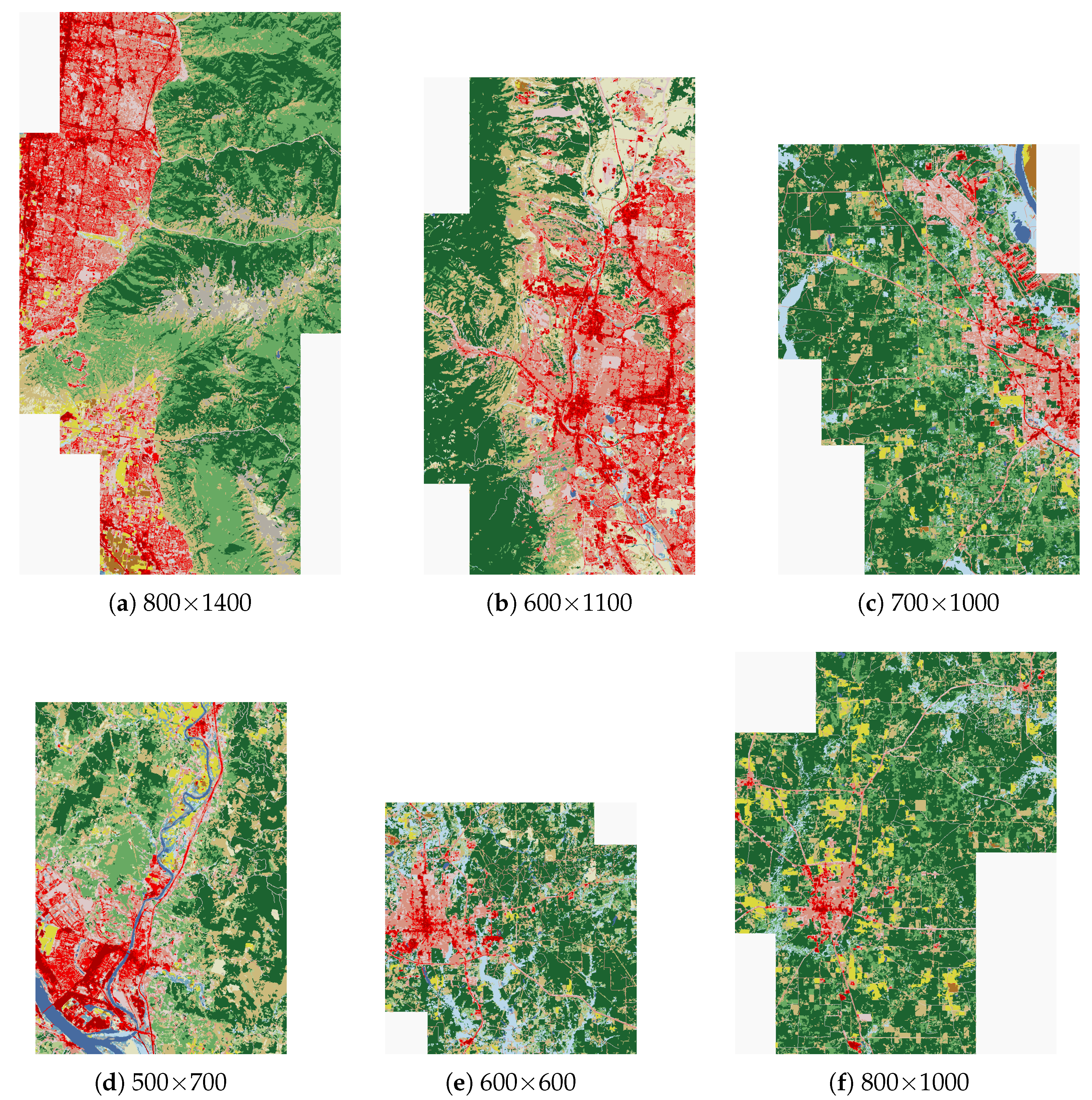
To demonstrate the validity of the proposed method, a number of comparison experiments were carried out. The whole database consists of a large landcover map with size pixels. We first divided the whole map into small patches of pixels without overlap. For the first three comparison experiments, two different scenes from the NLCD 2006 data set were chosen as the reference scenes. We adopted an overlapping sliding window with a size 500 × 500 pixels, where each time the window slid 100 pixels in either the horizontal or vertical direction. Since the NLCD database is of 30 m/pixel spatial resolution, each window covers 15 km × 15 km on the ground. With regard to the final experiments, we tried to retrieve the scenes containing an airport.
The first scene selected was in the region located in Kaufman Country, Texas (see
Figure 4). As we can see, the first reference scene is traversed by the Cedar Creek Reservoir, which is classified as “open water”. This could be the most noticeable information to determine the similarity between the reference and the retrieved scenes. Along the reservoir, there are a few classes belonging to the “developed” category. In addition to the “open water” and “developed” categories, the other two land-cover types of “pasture/hay” and “deciduous forest” occupy most of the remaining regions of this scene. The results of the retrieval experiment acquired by the use of the proposed method and the method proposed in [
28] are shown in
Figure 5 and
Figure 6, respectively. The scenes ranking first acquired by both methods are the same, and are in the same area where the reference scene is located.
Figure 5 and
Figure 6 reveal that the ranking order of the proposed method is more reasonable than the of the method proposed in [
28]. Judged only from the visual aspect, the last two scenes retrieved by the method proposed in [
28] are quite different from the reference ones. The first four scenes (including the first retrieved one) retrieved by the proposed method are very similar to the reference ones. In
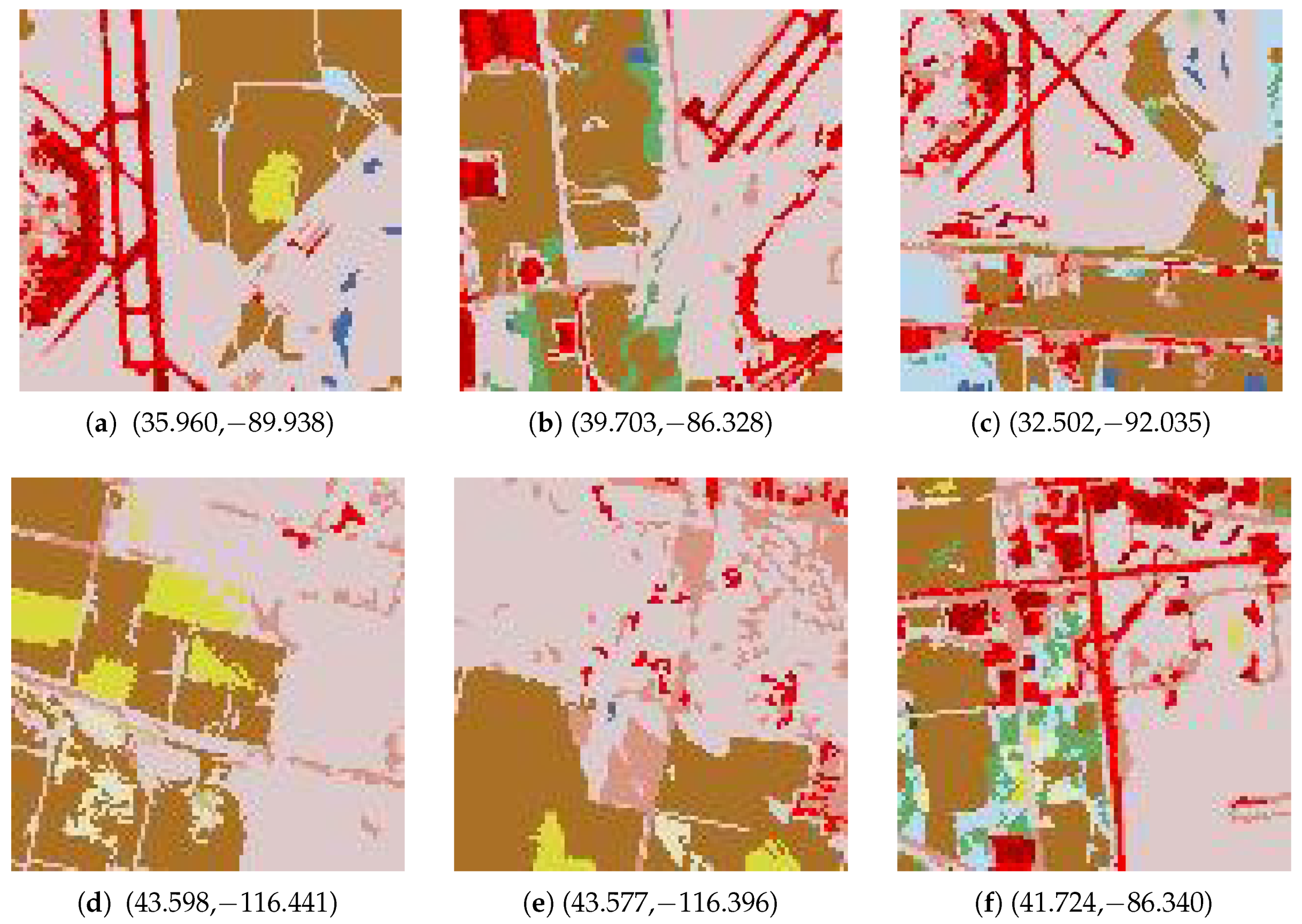
Figure 7 and
Figure 8, the remotely sensed images correspond to the retrieved scenes shown in
Figure 5 and
Figure 6. The images were acquired from Google Earth, using the geographical coordinates shown in
Table 1.
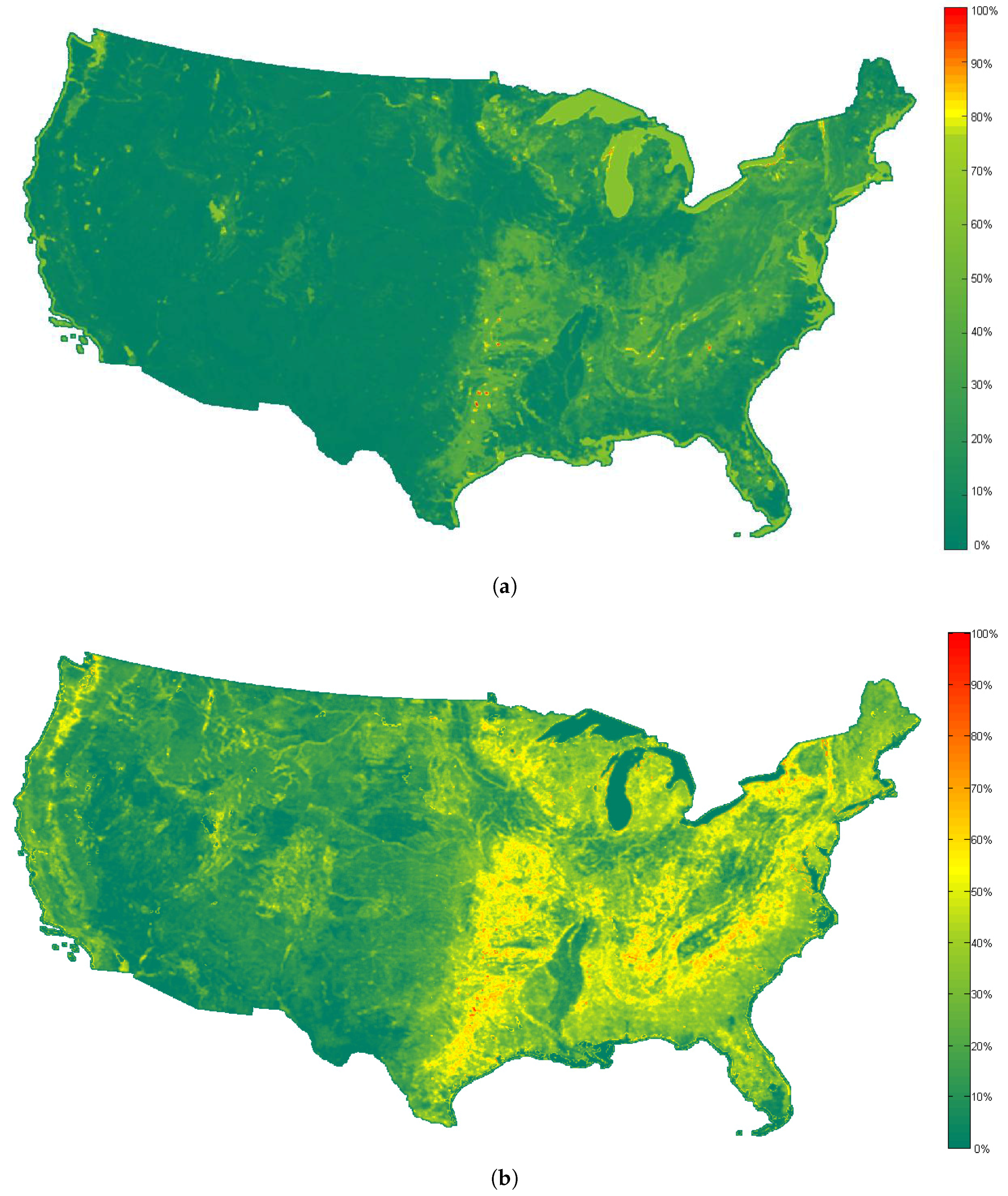
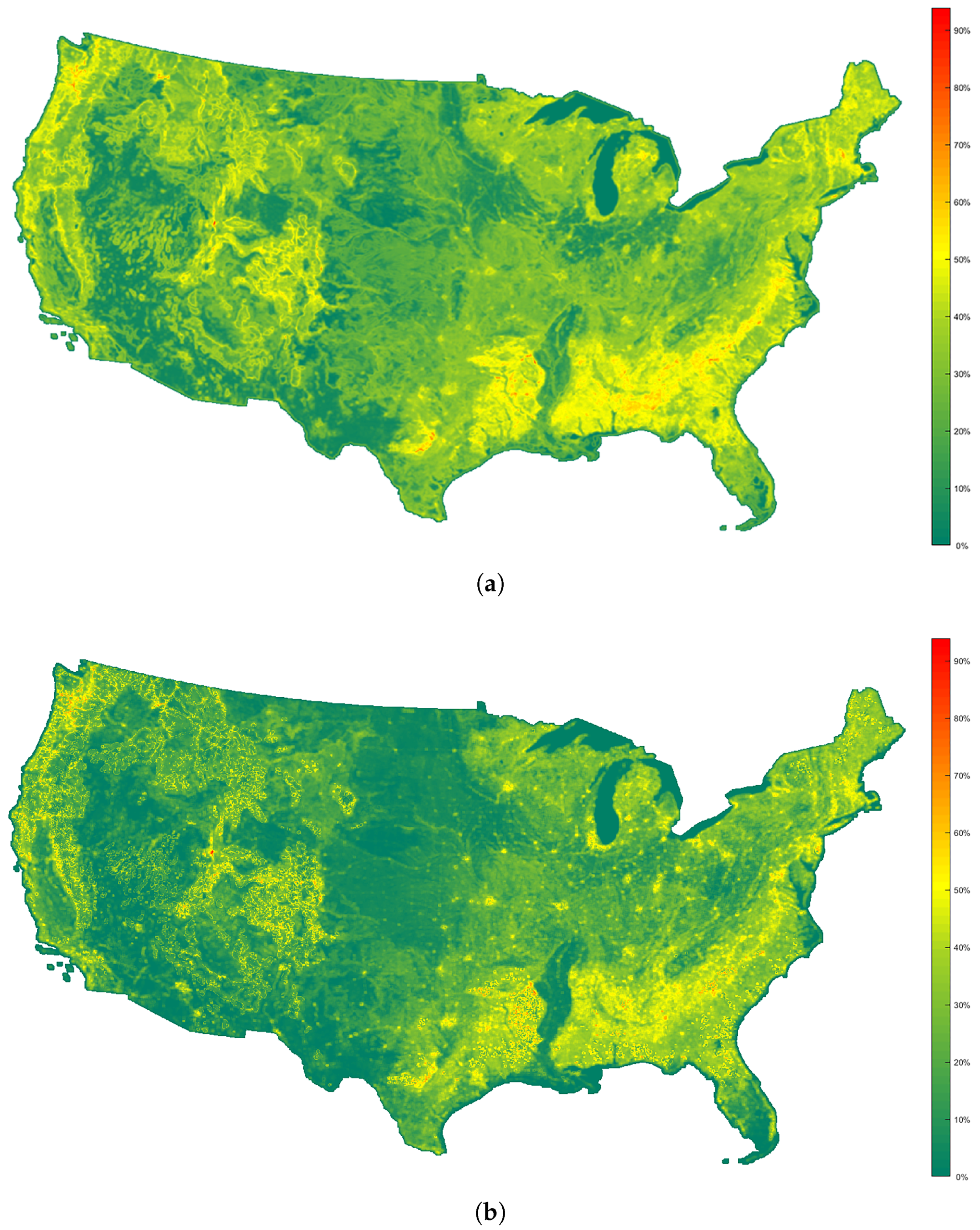
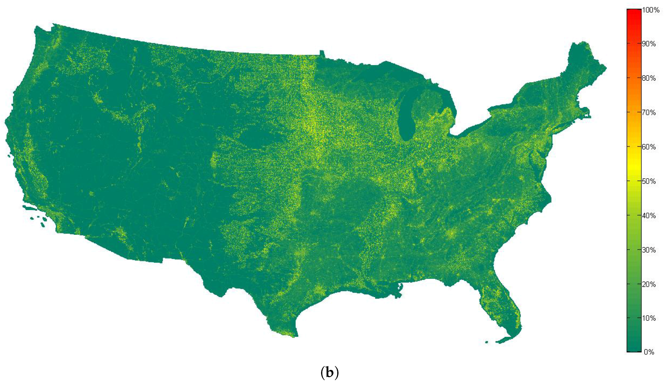
The most useful scene retrieval results are the similarity maps of the whole dataset compared to the reference scene. In
Figure 9, the similarity maps computed by the use of the proposed method and the method proposed in [
28] are shown.
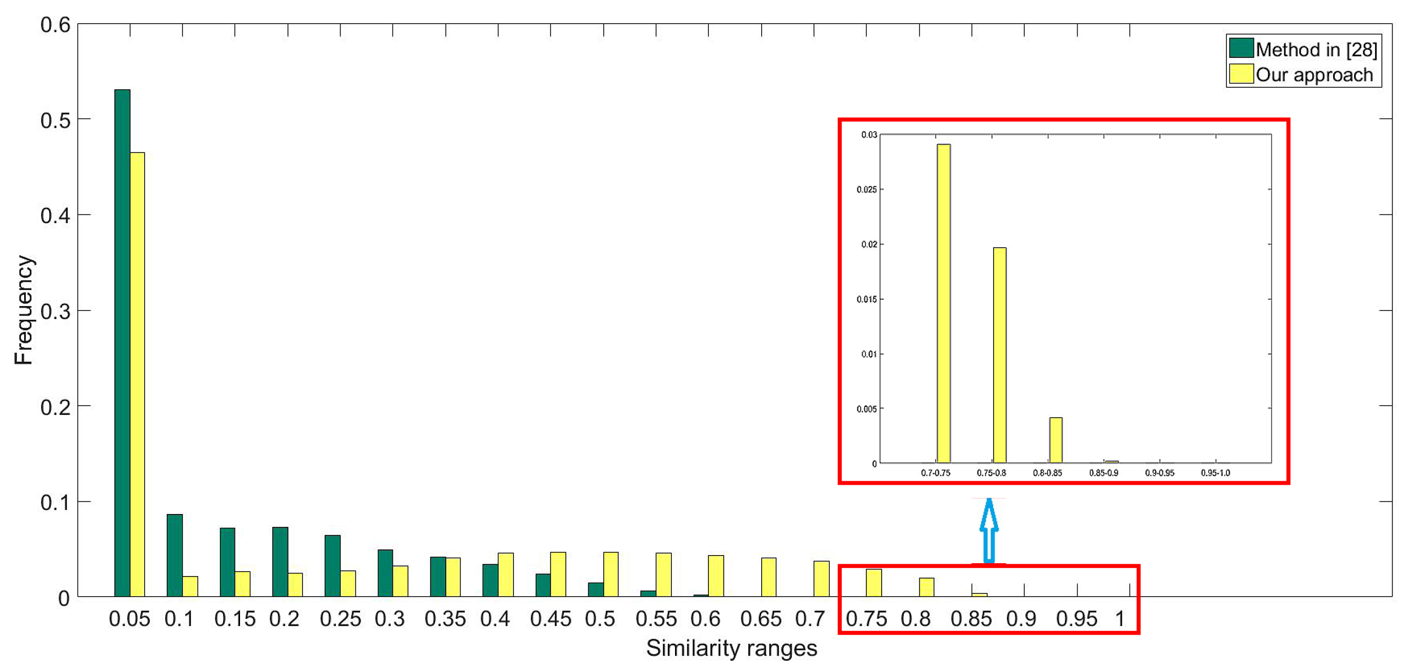
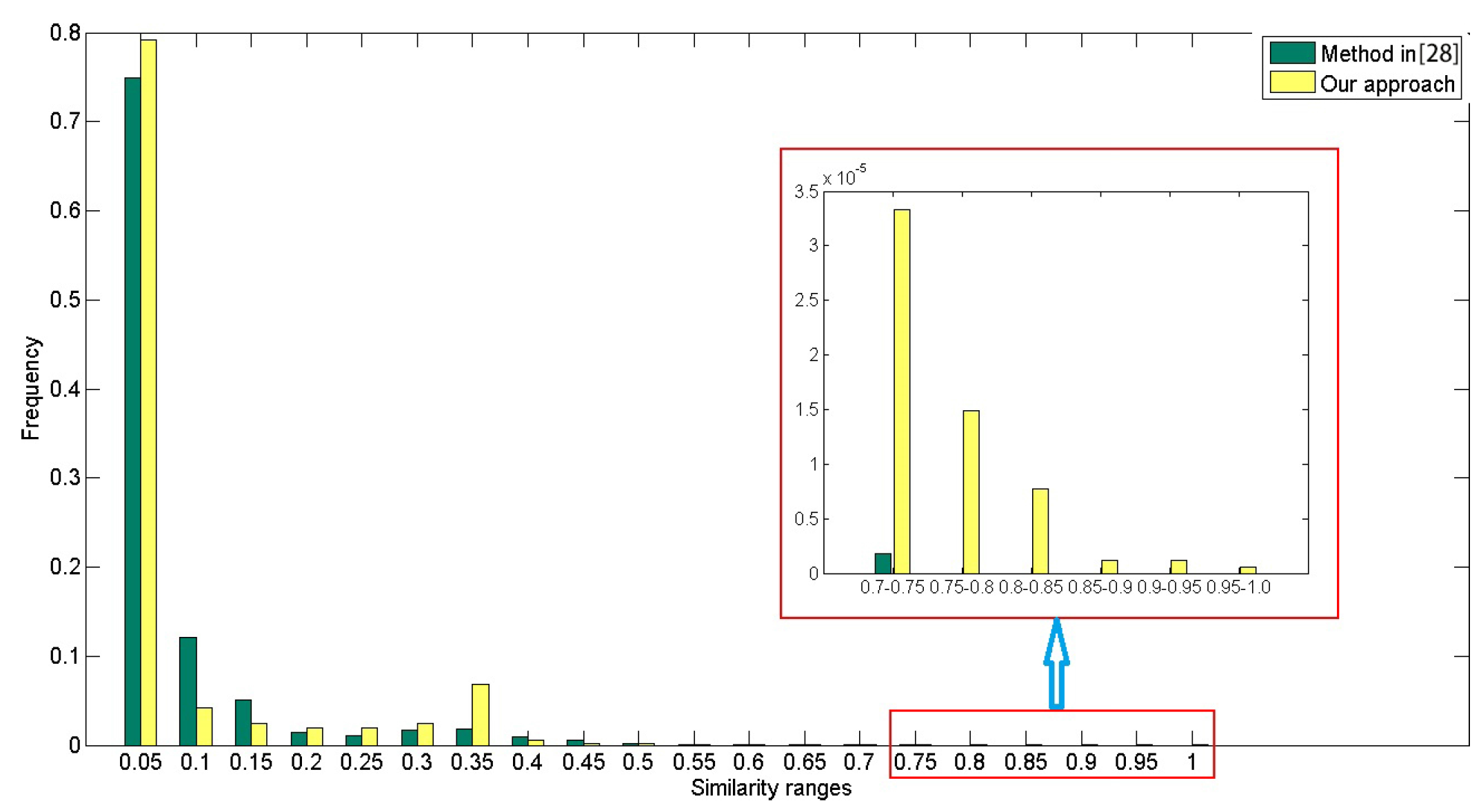
Figure 10 shows the histograms of the similarity maps in
Figure 9. It can be seen that although the visual aspects of the two similarity maps are different, high values of similarity measurements are always rare in both maps. In addition, the spatial distributions of both maps are correlated (i.e., the locations which have high values in
Figure 9a also have high values in
Figure 9b). However, according to
Figure 5 and
Figure 6, the rank order of the most similar scenes obtained by the proposed method seems more reasonable, which can help the user to obtain the desired scenes from the large database more efficiently.
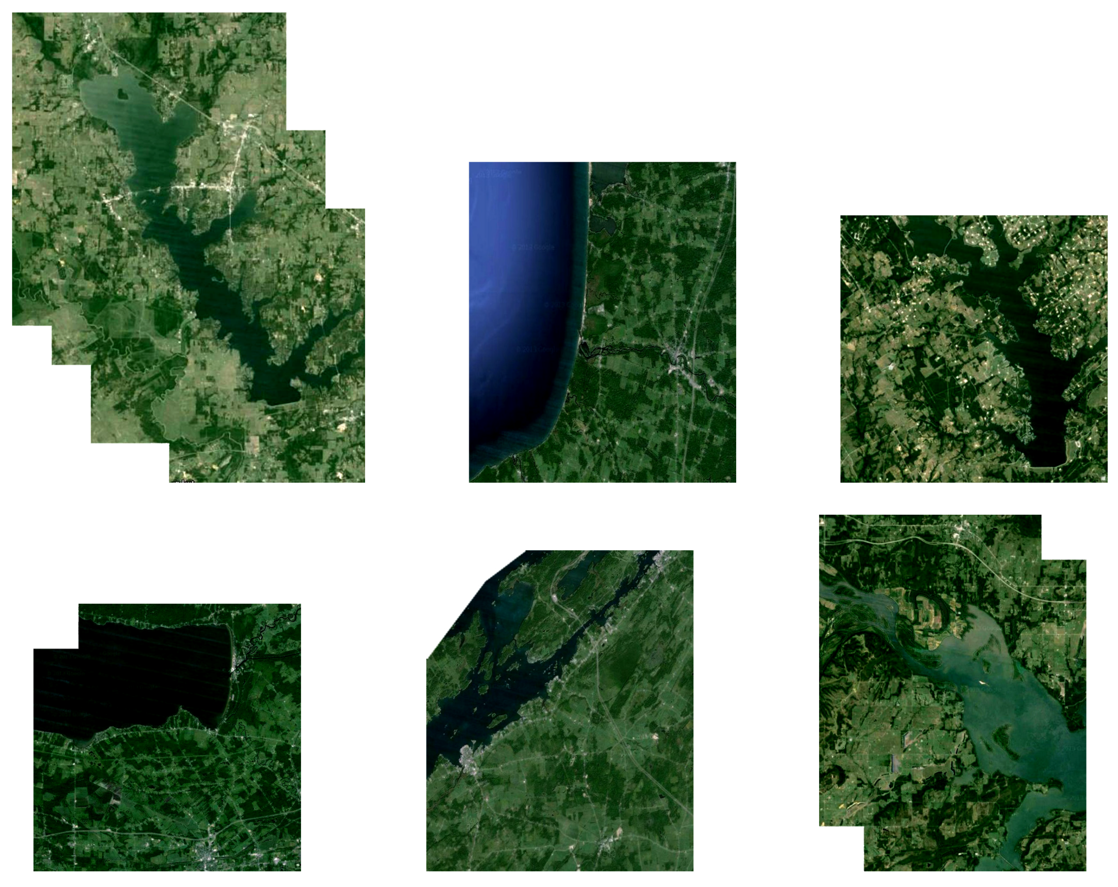
The second reference scene considered in our experiment covers Yucatan Lake, which is located in the northeastern part of the U.S. state of Louisiana (
Figure 11). The center of this scene is crossed by the Mississippi River, and the western part is divided into two parts by Lake Bruin—both of which are classified as “cultivated crops”. Both the Mississippi River and Lake Bruin are classified as “open water”. Both sides of the Mississippi River are covered with “woody wetlands”, and “deciduous forest” occupies almost the whole southeastern part of the reference scene.
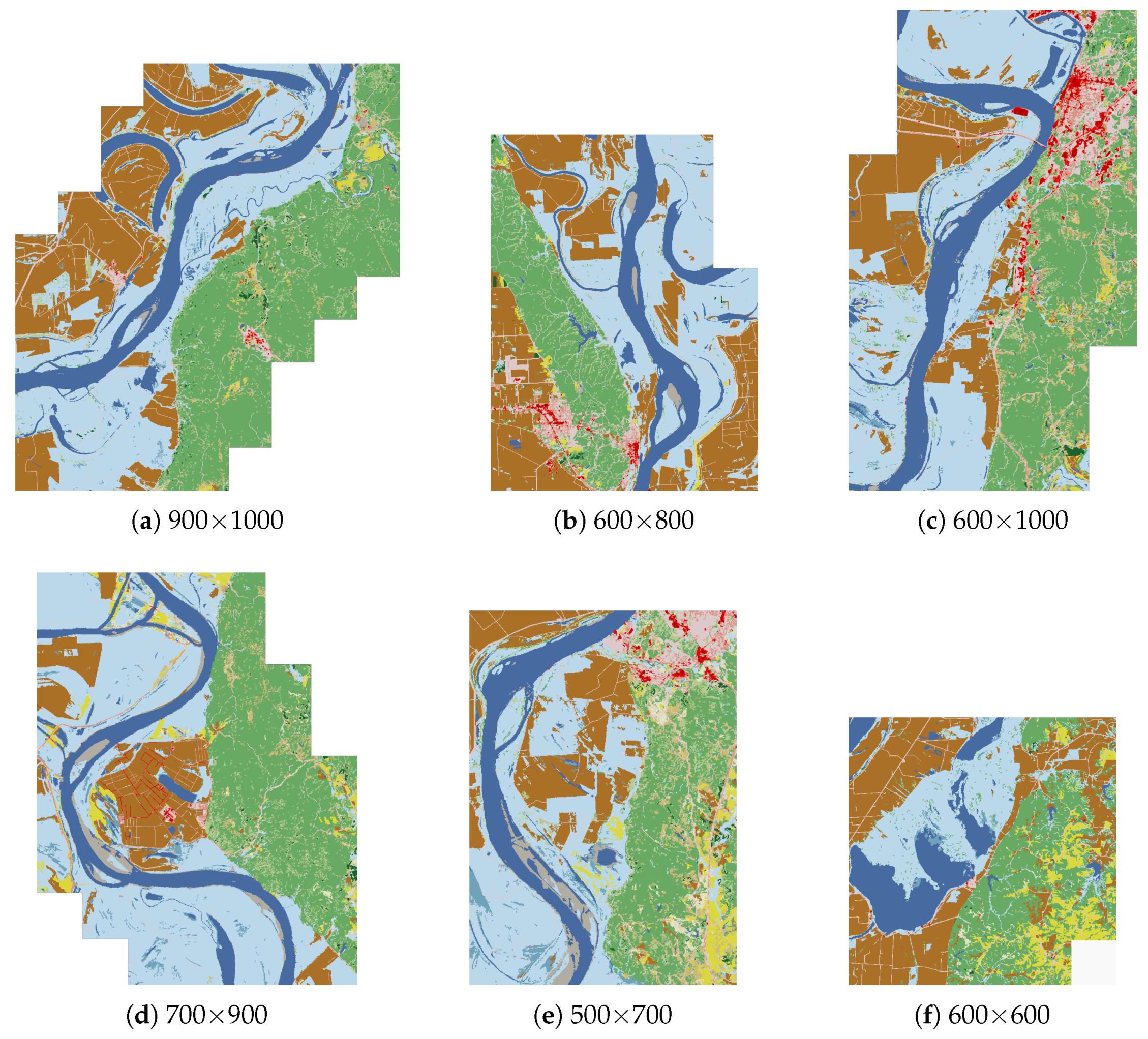
Figure 12 and
Figure 13 show the results of this retrieval. The geographical coordinates of the retrieved scenes are presented in
Table 2. The top five scenes given by the method proposed in [
28] are all included in the results of the proposed method, except that the ranking order of the scenes is different, and the size of the scenes also varies. Again, the similarity maps obtained by the two methods (see
Figure 14) are spatially correlated.
Figure 15 shows the histograms of the similarity maps in
Figure 14. However, the ranking order of the results is better when using the proposed method. The last scene obtained by the method proposed in [
28] (
Figure 13f) has different content.
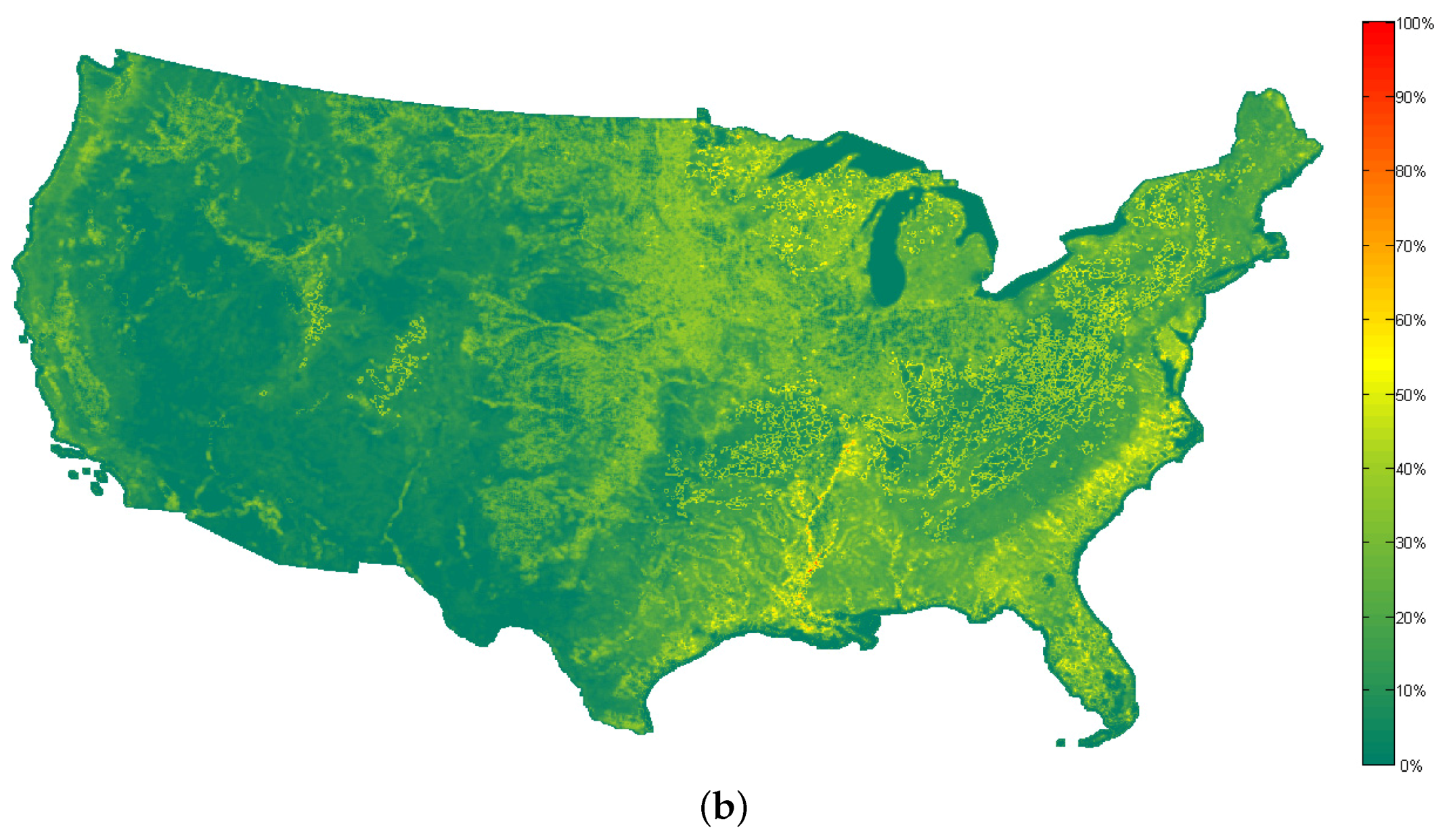
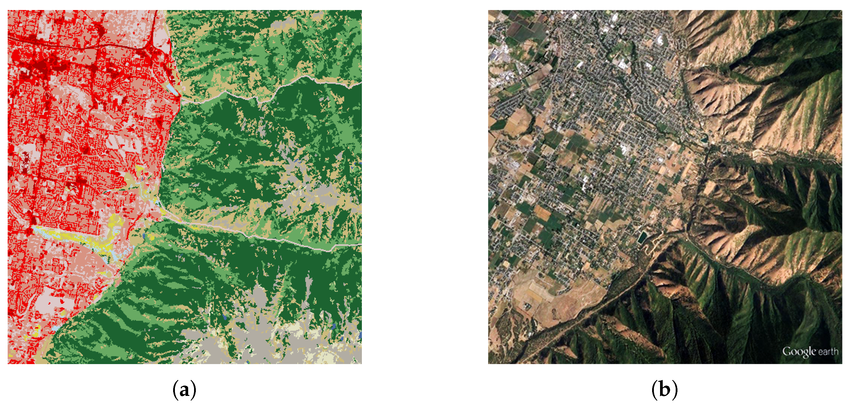
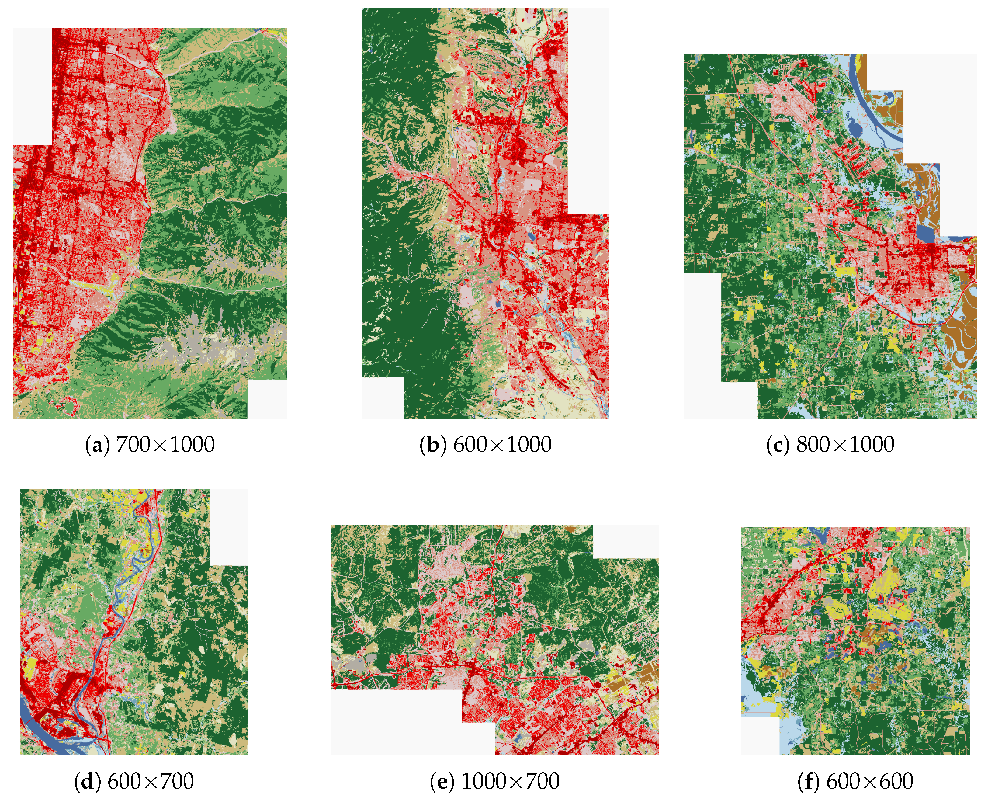
The third reference scene we selected is located in the northeastern part of the American state of Utah (
Figure 16). The upper part of the reference scene is located within Springville, while the majority of the reference scene is located within Mapleton. Compared to the two previous scenes, the third reference scene is more heterogeneous. Seen from
Figure 16, the western parts of the reference scene are urban areas, and the eastern parts are mountainous areas. The western parts are almost occupied by “developed” category with different intensities. Apart from the “developed” category, the other land-cover type “pasture/hay” occupies the remaining regions of the western parts. Within the eastern parts, the most common land-cover types are “evergreen forest”, “deciduous forest”, “shrub/scrub”, and “barren land”, which are typical landscape of the mountains.
Figure 17 and
Figure 18 show the results acquired by different methods. The geographical coordinates of the retrieved scenes are presented in
Table 3. The top four scenes given by the method proposed in [
28] are the same as the results of our proposed method, and the ranking order of the scenes are also identical, except that the size of the scenes varies. For the last two scenes (see
Figure 17 and
Figure 18) retrieved by each method, judged from the visual aspect, scenes acquired by the proposed method are much more similar than [
28]. The distribution of areas with relative high similarity are identical in
Figure 19a,b. So, the similarity maps obtained by the two methods (see
Figure 19) are spatially correlated.
Figure 20 shows the histograms of the similarity maps in
Figure 19.
In the last experiment, we tried to extract scenes with concrete semantics from the NLCD database. Due to the coarse resolution of the NLCD dataset (30 m), few ground objects are visible. It was observed that the airstrips in the NLCD 2006 dataset are usually represented by developed areas of medium and high intensities. We also observed that the neighbourhood regions of the airstrips are always filled with open space. Based on this information, we could try to retrieve scenes containing an airport.
A scene (see
Figure 21a) containing Arkansas International Airport was selected as the reference scene. We set the size of the sliding overlapping window as
pixels and the step size as 100 pixels.
Figure 21 and
Figure 22 show the top 12 similar scenes by each method. Apart from the similarity map (
Figure 23) and histograms of the similarity maps (
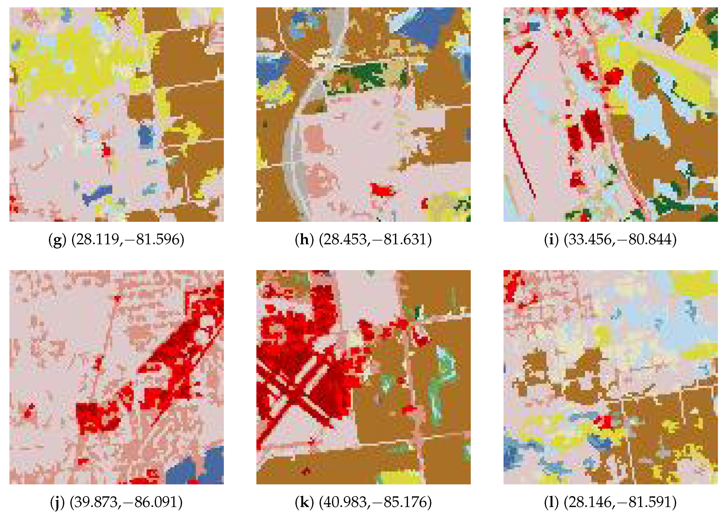
Figure 24), we also returned the ranking of the similarity degree. Therefore, we could also observe each scene from the top-ranking scene to the bottom. In order to give an authentic look to the scenes, rather than classified map, the geographic coordinates of each scene were returned. This allowed us to locate the scenes in Google Earth. Among the top 12 most similar scenes, there are six scenes (see
Figure 21a–c,e,i,k) containing an airport, which respectively correspond to Arkansas International Airport, Indianapolis International Airport, Monroe Regional Airport, South Bend Airport, Salina Municipal Airport, and Valley International Airport. Meanwhile, by the use of the method proposed in [
28], only three airports—Arkansas International Airport, Orangeburg Municipal Airport, and Fort Wayne Municipal Airport (
Figure 22a,i,k)—were returned among the top 12 scenes. Furthermore, we compared the precision of the top 96 scenes retrieved by the use of the proposed method and the method proposed in [
28]. The proposed method could obtain 29 airports, while the method proposed in [
28] could only acquire eight.
4. Discussion
We propose a CBIR-like remotely sensed scene retrieval system for use with LULC databases in this study. Motivated by GLCM, we propose a scene signature extraction method for LULC scenes. To validate our method, four reference scenes are selected to conduct the comparison experiments. For the first three reference scenes, we evaluated the performance of our method in two aspects: the content of the retrieved scenes, and the ranking order. As depicted in
Figure 5,
Figure 6,
Figure 12,
Figure 13,
Figure 17 and
Figure 18 that scenes returned by the proposed method seem much more similar compared to [
28]. Additionally, the rank order of the most similar scenes obtained by the proposed method seems more reasonable, which can help the user to obtain the desired scenes from the large database more efficiently. For the last reference scene, we selected a scene containing an airport. Among the top twelve most similar scenes, our method can return six scenes containing an airport, while [
28] had only three. Furthermore, we compared the precision of the top 96 scenes retrieved by the use of the proposed method and the method proposed in [
28]. The proposed method could obtain 29 airports, while the method proposed in [
28] could only acquire 8.
To achieve a finer retrieval result, we propose the LCM as scene signature. Through the designed CBMR, the user could obtain not only the alike scenes in varied scales, but also the similarity map. Moreover, the geographical coordinates of the alike scenes are also presented. Due to this, the scenes could be easily located in Google Earth or other map tools. Per the results mentioned above in
Section 3, the proposed method could achieve better performance. The retrieval result of the proposed method is more accurate and reasonable. Some future work is also expected. At first, the proposed method can be extended to ordinary remotely sensed images rather than land cover products. A rough classification of the images in order to convert the grey-valued (or multi-spectral) images into label images is required before the retrieval. In addition, we need to merge the feedback technique into our system. With relevance feedback technique involved, users would be able to indicate to the image retrieval system whether the retrieved results are “relevant”, “irrelevant”, or “neutral”. Retrieval results would then be refined iteratively. This could help the user obtain much more accurate results. The next aspect we need to take into consideration is the complex semantic information; for example, a large open space with many cars is likely to be a parking lot.


