2.1. Study Population
A commercial weight loss program offering clinically impactful behavioral support provided weight data for unrestricted use to Tufts University (Instinct Health Science,
www.theidiet.com, accessed on 11 April 2024). The iDiet was developed by co-author SBR, and detailed descriptions of this program are given elsewhere [
23,
24]. In brief, the iDiet program targets a weight loss of 0.5–1 kg of weight per week by reducing energy intake by 500–1000 calories per day. In addition, it has the specific goal of reducing hunger and food cravings by providing menus and recipes relatively high in dietary fiber and protein and low in energy density and carbohydrate glycemic index. Each program block was 11 weeks long, but individuals could choose to continue with one or more additional blocks. Each 11-week program was implemented as a small group program that met once a week for an hour to learn about nutrition and weight management, discuss it, and support one another. Participants were encouraged but not required to enter their weight records via the program website. The analysis of the iDiet data was approved by the Institutional Review Board at Tufts University.
The original dataset comprised 305,248 weight records from 2520 participants who were enrolled in the program between 2012 and 2019. To ensure data quality, we conducted initial data screening by excluding records based on the following criteria: (1) weight records without reporting the type of unit (kg or lb.), (2) weight values recorded as 0, and (3) weight values lower than 40 kg or higher than 250 kg. Subsequently, the screened dataset contained 302,373 weight records from 2494 participants. For algorithm development and subsequent analysis, we focused on participants who recorded their weight for at least 11 weeks (77 days) and limited the duration between the first and last records to at most one year (365 days), even if they recorded weight for over one year. Additionally, we excluded participants if two consecutive weight records were more than 30 days apart and if they recorded fewer than five weights throughout their program participation. These selection criteria resulted in a study sample of 667 participants, with a total of 69,363 weight records. The process of data selection is depicted in the consort diagram (
Figure 1), and comprehensive summary information for both the original and the study sample is given in
Table 1. We did not include gender, age, and height information in our data analysis, as these variables had more than 40% missingness in the original datasets, which resulted in less than 50% of participants with complete demographical data. Detailed summary statistics of age and sex information are listed in
Table 2.
2.2. Sequential Modeling
We employed a sequential polynomial regression modeling approach to analyze individual weight trajectories. This involved fitting three models for each trajectory, starting with a linear term, followed by the addition of a quadratic term, and finally incorporating a cubic term. The model equations for the linear (m
1), quadratic (m
2), and cubic (m
3) models are presented below:
where
represents the weight value for
i-person, recorded on
t-day from the start of individual recording, with
t ranging from 1 to the last day (
) of recording of each participant;
β0,i represents the intercept for the
i-person,
β1,i represents the coefficient of the linear term
t for the
i-person,
β2,i represents the coefficient of the quadratic term
t2 for the
i-th person, and β
3,i represents the coefficient of the cubic term
t3 for the
i-person; ε
i is the error term in the model for the
i-person.
2.3. Weight Trajectory Classification Algorithm
The first step in classifying weight trajectory is to determine the optimal model for each participant. We extracted the adjusted R2 of the linear, quadratic, and cubic models to compare the models’ performance for each individual trajectory. A threshold of a 5% change in adjusted R2 was applied to assess the superiority of a more complex model over a simpler one. If the percentage change in adjusted R2 when comparing the more complex model to the simpler model exceeded 5%, we considered the trajectory to be better fitted by the more complex model. Conversely, if the change did not surpass the 5% threshold, the trajectory was classified using the simpler model.
Subsequently, we estimated a set of key parameters to facilitate further classification: Total duration is denoted as , where t1,i and tz,i represent the first day and the last day of weight recording for the i-person.
Predicted weight values on the first day are denoted as , , , and on the last day are denoted as , , , for model m1, m2 and m3, respectively.
For a quadratic model m
2, the nadir point of the trajectory curve is calculated as:
The predicted weight at the nadir is denoted as .
For a cubic model m
3, the Δ of the derivative of the cubic model is calculated as:
When Δ > 0, there are two vertex points,
and the predicted weight of the two vertex points are
and
, respectively.
After the participant data were grouped into the optimal models, we developed different criteria for the linear, quadratic, and cubic models, respectively, by applying those key parameters above together with the model coefficients to further group participants’ trajectories according to the shape of the individual trajectories. Detailed descriptions of the criteria are listed in
Table 3.
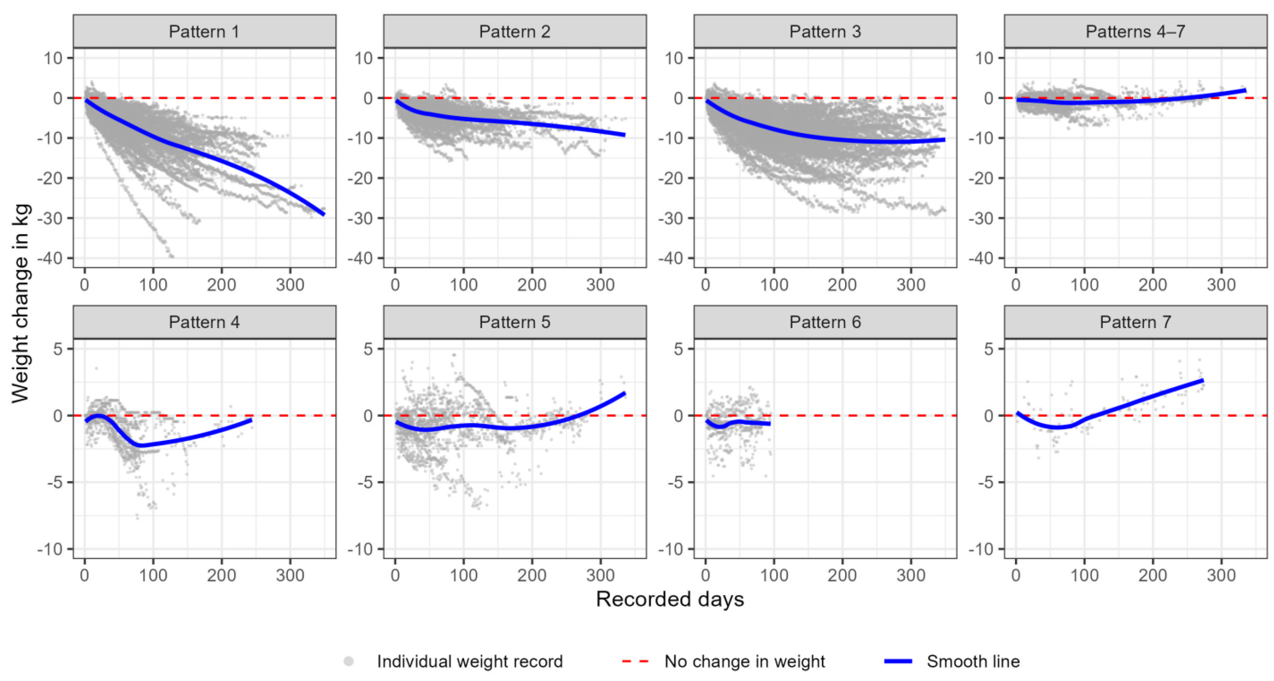
Next, we created a multi-panel scatter plot to visually compare the similarities within the same pattern and the differences among different patterns. The scatter plot depicted the individuals’ weight change compared to their previous weight records over time, from the participant’s first day of records and up to one year. The participants classified into the same pattern were grouped into the same panel, so the different panels represented different weight trajectory patterns. The points on the scatter plot are the individuals’ weight records. We also added a Loess smooth curve to each pattern to represent the overall weight change pattern over time. To enhance the utilization of our sequential modeling and its associated parameters, we developed a growth chart-style plot that incorporates additional percentile lines. These percentile lines, namely the 1st, 5th, 10th, 25th, 50th, 75th, 90th, 95th, and 99th, are dynamically determined based on the values of the model coefficients within each pattern. This visualization effectively portrays the predicted weight trajectory over a 14-week period in seven distinct patterns.
2.4. Early Prediction Modeling
To examine the association between weight change rate in the first 14 days and the individuals’ trajectory patterns, we applied a multinomial logistic regression adjustment for the number of records in the first 14 days and the total participated durations.
where
j represents a defined weight trajectory pattern, and
j = 1,
X1,i represents the weight change in the first 14 days (difference divided by 14 days), X
2,i is number of records collected in the first 14 days, and X
3,i is the duration, or the number of participated days for
i-participant.
To examine if early weight change characteristics differ in different trajectory patterns, we extracted the estimates of beta coefficients and standard error from the model output for each pattern compared to a reference, Pattern 1, and exponentiated model coefficients to calculate the odds ratio and 95% confidence interval. The odds ratio estimates the ratio of the likelihood of being in one pattern to the likelihood of being in a reference pattern for every one-unit increase in weight change rate in the first 14 days, adjusting for the number of records in the 14 days of the total participated duration. To improve the model sensitivity, we combined the patterns with low representation.
2.5. Model Validation and Sensitivity Analysis
To validate our sequential model, we employed 10-fold cross-validation across all the linear, quadratic, and cubic models. The data were randomly partitioned into 10 equal-sized folds, with 9 folds used for training the model, and the remaining fold used for testing. This process was repeated 10 times, with each fold as the testing set once. We report the root mean squared error (RMSE), and R squared as our primary performance metric. To evaluate the robustness of our classification methodology, we conducted sensitivity analyses. These analyses involved varying the threshold number of classification criteria to examine the stability of the participants’ weight trajectory groupings. Specifically, we tested threshold values 0.5, 1.5, and 2 for C1.1, C2.1, and C3.1, values 1.5 and 2.5 for C2.4, and 2.5 and 3.5 for C3.7. The percentage of the participants who changed their weight trajectory groups was represented as the sensitivity metric. We further conducted a sensitivity analysis to assess the potential impact of age and sex on the prediction model. We additionally included the variables age and sex in the model and compared the change of coefficient among other predictor variables.
All the statistical analyses were conducted using R version 4.2.0. ANOVA was employed to test for differences among groups. Tukey’s honestly significant difference test was used to determine pairwise differences between groups. Statistical significance was established at p < 0.05.


