1. Introduction
Ultrathin nanopores are artificial apertures of nanoscale dimensions on sub-
inorganic membranes [
1]. In comparison with biological pores on protein membranes, these pores possess unrivaled advantages of flexibility in dimensions, mechanical robustness, and chemical stability, and hence stimulate the development of frontier technologies for versatile applications [
2]. Utilizing a two-dimensional (2D) material, monolayer molybdenum disulfide, Feng et al. [
3] demonstrated extraordinary energy conversion performance of reverse electrodialysis when converting a salinity concentration difference into electricity. Paul et al. [
4] blueprinted a nanopore-based bubble emitter for cooling applications in closely packed electronic components in response to the rising demands of high-performance computers. As viruses electro-migrate through nanopores, their structures and charge conditions can be identified by detecting the ionic current variations [
5], which is imperative for medical diagnosis in society after COVID-19.
To further pursue the improved performance and accuracy of these applications, it is vital to examine the ion and flow behaviors in ultrathin nanopores from a fundamental perspective. When these nanopores are immersed in an electrolyte solution, the positively/negatively charged surface results in the selectivity of ions that renders higher penetration of anions/cations over their counterparts, as long as an electric potential difference is present across the membrane. This ionic selectivity causes a slight salinity concentration imbalance between the two sides of the membrane, known as ion concentration polarization (ICP) effects [
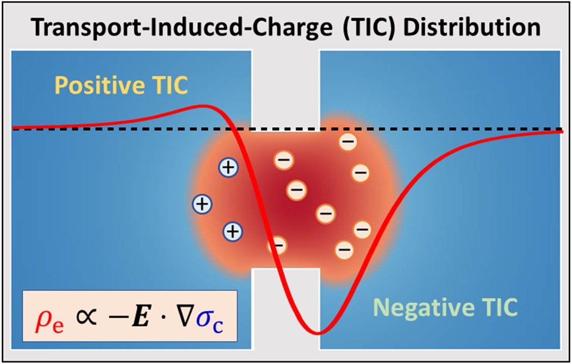
6]. In other words, the axial electric potential gradient induces an axial concentration gradient due to the radial electric field induced by the surface charge. The magnitude of these gradients is determined by the concentration of bulk salinity, applied electrical potential difference, and thickness of the membrane. As the membrane becomes considerably thin, the interaction between the strong electric field and the steep concentration gradient promotes local ion separation, resulting in a net space charge outside the electrical double layer (EDL). This phenomenon, known as transport-induced-charge (TIC) effects [
7], disturbs the ionic distributions in the nanopores and considerably influences the electroosmotic behavior.
TIC effects due to the coexistence of an electric field and a concentration gradient were theoretically reported by Rademaker et al. [
8] in an electrochemical system of lithium-ion batteries. However, although the induced charge could occur in their system, it was negligible compared to the bulk ion concentrations. On the contrary, in ultrathin nanopores, both the electric field and the concentration gradient are focused and amplified within a nanoscale dimension, yielding significant TIC effects that influence nanopore electrokinetics. Hsu et al. [
7] investigated the behavior of electroosmotic flow (EOF) caused by TIC (TIC EOF) via computational simulation. The results indicated that the TIC EOF is dominant at the high applied electric potential difference (
) compared with the conventional electroosmotic flow originating from the EDL (EDL EOF). Thus, the TIC EOF can reverse the flow direction when the applied electric potential difference exceeds a certain critical value. This unique phenomenon properly explained the anomalous DNA translocation behavior observed by molecular dynamics in a previous study [
9], in which a threshold voltage was required to drive DNA molecules through a 2D nanopore in order to overcome the opposing EDL EOF.
In the model of Hsu et al. [
7], it was assumed that the system maintained an isothermal condition and the simultaneous Joule heating effects produced by the applied electric field were not considered. However, this assumption cannot remain valid for the cases at high applied voltages. For instance, Nagashima et al. [
10] demonstrated homogeneous bubble formation activated by superheating in nanopores attributed to Joule heating effects when an extra-high voltage was imposed (e.g.,
). The existence of a non-uniform temperature results in overlapping of triple effects (temperature gradient, salt concentration gradient, and electrical field) within a small distance in ultrathin nanopores, which could lead to intricate electrokinetic behavior. In this study, we theoretically investigate the coupling of Joule heating effects with TIC phenomena via computational simulation. Thus, the variation in the TIC in response to the localized temperature rise can be controlled. In addition, the impact of TIC on the electroosmosis behavior is evaluated, which may enrich our understanding of complex electrokinetic phenomena in ultrathin nanopores.
2. Computational Modeling
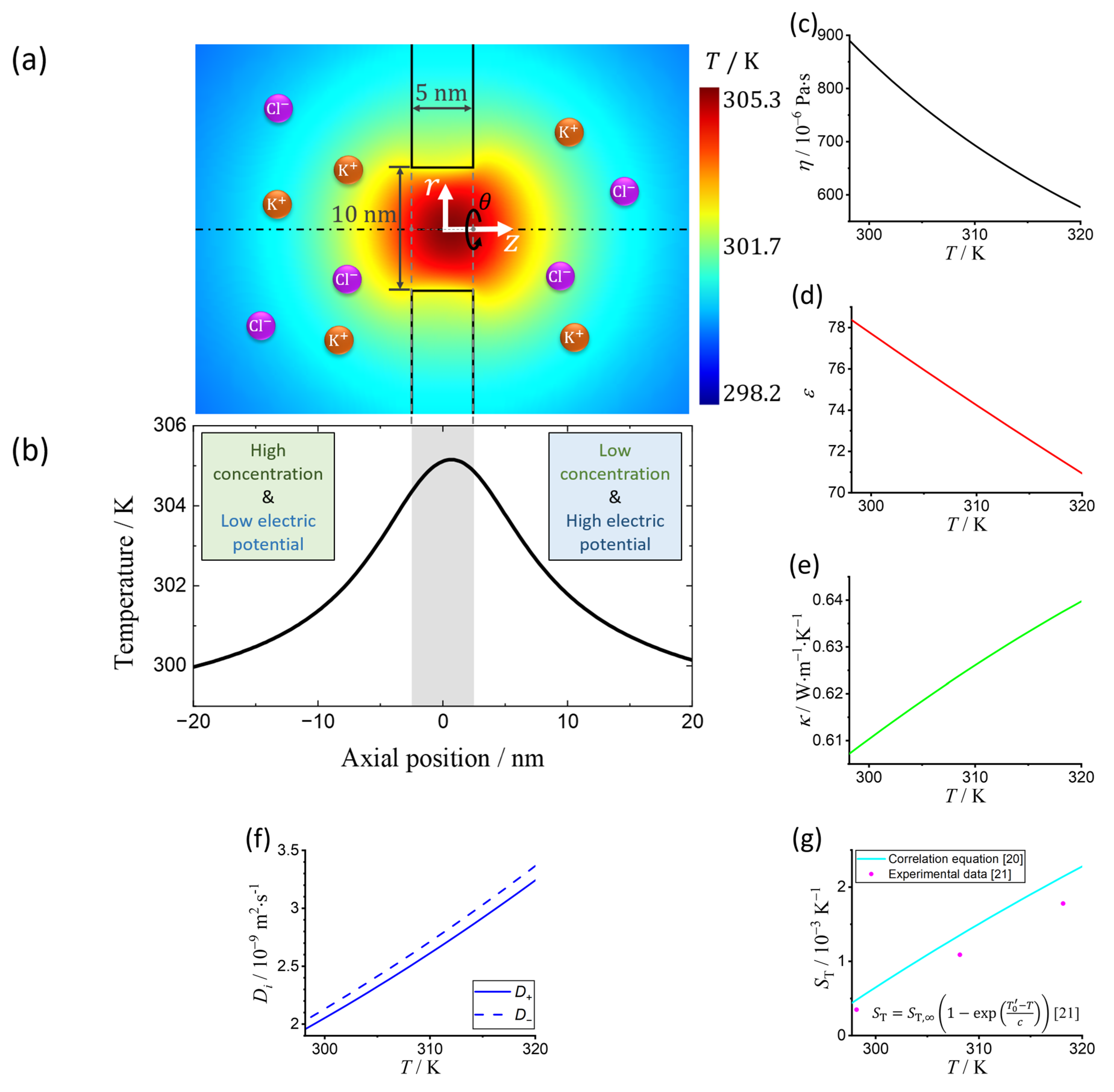
A steady-state model of Joule heating effects on TIC phenomena in an ultrathin nanopore in a 2D cylindrical coordinate is investigated. As illustrated in
Figure 1a, a nanofluidic system with a silicon nitride (SiN) nanopore (
thick and
in diameter) filled with asymmetrically concentrated potassium chloride (KCl) aqueous solutions from each side is considered [
11,
12,
13]. Then, an external electric field is applied parallelly to the salt concentration gradient. The midpoint of the nanopore is set as the origin
O, an arbitrary radial direction as the polar axis
, and the central axis of the nanopore as the cylindrical axis
. Accordingly, a 2D cylindrical coordinate system
is employed, and the system is symmetric with respect to the azimuthal
-direction.
By considering mass conservation, we adopt the continuity equation for the solution at steady state:
where
is the velocity vector of the solution. Note that although the solution density
depends on the solute concentration and temperature, the concentration of water molecules (~55.6 M) is considerably higher than the solute concentration, making the density barely change with the amount of KCl dissolved. In addition, between 25–99 °C the density variation of pure water is less than
[
14]. Thus we assume that
is constant in the system (i.e., incompressible fluid), equal to the density of pure water.
The typical axial temperature distribution in this flow system is shown in
Figure 1b. Due to the huge difference between the concentrations of solvent and solute, the temperature-dependent solution properties are also replaced by pure water properties as shown in
Figure 1c–e, the solution properties, including the viscosity
, static dielectric constant
, and thermal conductivity
, are considered from previous experimental results of pure water, which are valid between
[
15] (detailed information is provided in the
Supplementary Materials Section S3). The specific isobaric heat capacity
is regarded as constant because its variation with temperature is less than
between
[
15], covering the temperature range in this study.
A modified steady-state Navier–Stokes equation considering the electric force on the electrolyte solution is used:
where
,
,
,
are the pressure, space charge density, electric potential, and absolute dielectric permittivity of classical vacuum, respectively. The variation in viscosity
[
16] due to the local electric field is not considered. The terms
and
are the electric body force on the free charges distributed in the solution and the dielectric force on the solvent due to the variation of
, respectively [
17].
The steady-state ion distributions can be described by the Nernst–Planck equation [
18], where the subscript
of “
” denotes the cation
and anion
, respectively:
where,
,
,
, and
are the molar concentration, diffusivity, mobility, and thermal diffusion coefficient of ions, respectively.
,
,
, and
represent the advection, diffusion, conduction, and thermodiffusion ionic fluxes, respectively. According to the Stokes–Einstein equation,
, where
and
are the ionic diffusivity and the viscosity of water at temperature
, respectively. We use
for
and
for
[
14].
generated from electrochemical migration is proportional to the ionic mobility
, where
and
are the elementary charge and Boltzmann’s constant, respectively. The variation of
as a function of temperature is shown in
Figure 1f.
arises from the Soret effect due to the presence of the temperature gradient, also known as thermodiffusion [
19]. The relation between the thermal diffusion coefficient and diffusivity is described as
, where
is the Soret coefficient, which is usually determined empirically. When
, thermodiffusion is from hot to cold regions, whereas
denotes thermal migration of ions from cold to hot regions. Here, we adopt an empirical correlation valid between
and
from a previous study, in which
, where
,
, and
[
20], measured at the KCl concentration of
. Note that these parameters are largely insensitive to the solute concentration at the currently investigated concentration level [
20,
21]; hence, we consider these parameters to be constant. In this regard, the relation between the Soret coefficient and temperature is plotted in
Figure 1g.
The electric potential distribution is described by the Poisson equation as below:
where
is the Avogadro constant.
The steady-state energy balance for the liquid electrolyte solution is described by Equation (5):
where
is the current density. The term
represents the heat source caused by the Joule heating effects and
can be obtained by the ionic flux as
, in which the advection ionic flux terms are not considered because they do not contribute to the relative velocity between the ions and the liquid [
22], despite their role on the current. It can be seen that the currents
formed by positive ions and
by negative ions of the system are also composed of four parts,
, in which the four terms on the right represent the contribution of the corresponding integrated ionic flux on the cross-sectional area of the system; for example
, in which the direction of the unit surface normal
is the same as the positive direction of the system. Viscous dissipation is not considered in this system because of its limited influence on the temperature rise compared to Joule heating effects (detailed information is provided in the
Supplementary Materials Section S2).
For the silicon nitride thin layer, the electric potential distribution is not considered, and the steady-state energy conservation equation is expressed as:
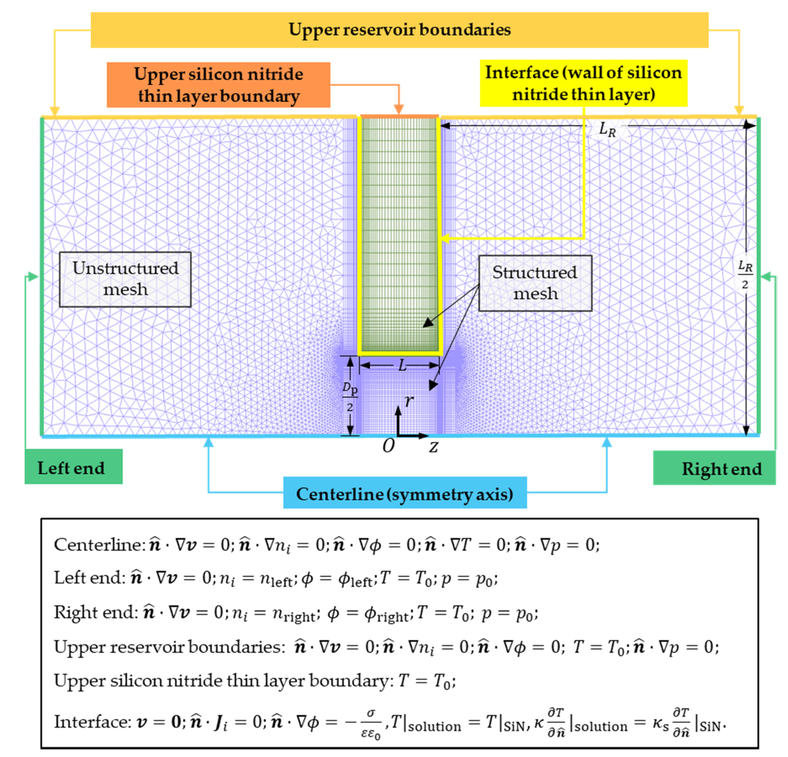
Figure 2 shows the axisymmetric 2D model with boundary conditions.
is the normal unit vector pointing outside (
is pointing toward the layer on the interface of the solution and the silicon nitride thin layer). On the centerline (along the
-axis), the pressure, velocity, concentration, electric potential, and temperature are satisfied with symmetry boundary conditions. At the far ends of the two reservoirs, the flow is considered to be fully developed with a constant concentration, temperature, electric potential, and pressure. A concentration bias
is applied to the two reservoirs such that the solution concentrations at the left and right far ends are
and
, respectively. Here,
is the average molar concentration of the solution. The temperature at the left and right end is maintained at
. An external electric potential difference
is applied between the right and left end of the system and
, where
and
are the electric potential of the right and left ends, respectively. Experimentally, one end of the solution is normally connected to ground as a reference electric potential. However, given that the electric potential is a relative quantity, the selection of the reference potential would not alter the physical phenomena. One can interpret that the reference electric potential taken here as the ground potential plus
(in the case when the low potential end is grounded). On the upper boundaries, the temperature is fixed at
and symmetry boundary conditions are applied for other unknowns for both reservoirs. At the interface between the silicon nitride thin layer and the solution, the nonslip boundary condition is adopted, the ion flux is zero along
, and the temperature and heat flux are continuous. The thermal conductivity of silicon nitride
is obtained from [
23]. The surface charge density
on the silicon nitride thin layer is related to the local electric field as [
24]:
Due to the deprotonation reaction of silanol groups on the surface,
can be affected by temperature due to the variation of the reaction constant. In the literature, the surface charge density at the silica/water interface subject to silanol groups at different temperature has been investigated both theoretically and experimentally. Close to room temperature, a previous theoretical study based on an electrical quad-layer model coupled with temperature effects [
25] shows that surface charge density increases less than approximately
when the temperature is elevated by
. Similarly, using sum frequency generation measurements, recent experimental results demonstrate that the increase of surface charge density due to temperature effects near room temperature is marginal [
26]. Therefore, according to the temperature range considered, we neglect the variation of surface charge density due to thermal effects in our modeling. However, a complex surface model may be needed for higher temperatures (
).
Continuum dynamics can describe the transport phenomena of ions in nanofluidic channels when the length scale is above
[
27]. The previous results of molecular dynamics show that the temperature gradient is continuous in the liquid phase at the quasi-atomic scale [
28,
29], thus verifying the continuous assumption including the temperature field inside our system. On this account, we solve the governing equations by numerical simulation, which is discretized in an implicit finite volume formulation [
30] on a hybrid mesh consisting of structured and unstructured grids. The length
of the reservoir in the computational domain is
, which can provide sufficiently accurate results that are not sensitive to the size of the reservoir and remain computationally efficient. Even if
is increased to
with a larger computational domain and more and denser mesh grids, the relative difference of the simulation results between these two cases is smaller than 2.5% (detailed information is provided in the
Supplementary Materials Section S1). The total cell number of the mesh is 149,004, including 100,086 unstructured triangles and 48,918 structured quadrangles.


 and
and 


