In this section, we will start with the description of the electromechanical and optical properties of the MAAM mirror. The parameters described here are further used as input parameters for the coherent system simulation model. This is followed by the description of the experimental setup, which resembles all important optical and mechanical properties of the coherent system simulation model. Having established methods to obtain simulative and experimental data to characterize the MAAM mirror, an approach to compare these data is introduced.
2.1. Design, Fabrication, Electromechanical and Optical Properties of the MAAM Mirror
The electromechanical design of the MAAM mirror consisted of a silicon membrane, suspended over an aluminum counter electrode, deposited on a fused silica chip (
Figure 2). The membrane acts as the MAAM mirror and exhibits the desired parabolic surface curvature variation when a voltage is applied between membrane and counter electrode. The basic concept of the cylindrical mirror, in which only the long axis is deformed parabolically whereas the short axis should remain as flat as possible, has been derived from a point-symmetric, round mirror design described in [
26]. Two design features are important to obtain a large aperture with a purely parabolically deformed optical surface: a so-called “soft” mechanical support of the membrane at the rim, which is realized by micromachined thin and narrow beams and an electrostatic force acting predominantly at the outer part of the deformable membrane. Additionally, because stress in thin layers is a critical aspect in any kind of deformable MEMS structure, wave front errors caused by stress-induced membrane distortions (e.g., out-of-plane buckling) must be addressed for the use of reflective focusing. To this end, the membrane suspension was designed in such a way as to allow for in-plane stress release and reduce out-of-plane buckling [
27].
Figure 2 schematically shows the cross section and top view of the working principle and design. The incoming collimated ray bundle is reflected to defined focus points, depending on the actual deformation state of the membrane. The focal length
f is given by the well-known relationship:
where
R denotes the parabolic radius of the membrane deformation [
28]. In contrast, ray bundles perpendicular to the parabolic profile, i.e., arranged in the plane direction of the membrane, are not focused by it.
The membrane itself is the deformable electrode. The fixed counter electrodes have a stripe-like design where the stripe length is perpendicularly oriented to the long axis of the membrane and the two stripes are placed below the two outer edges of the focusing Si-plate, which is deformed parabolically. Thus, the electrostatic force for the deformation of the membrane acts predominantly at the outer rim of the long side. To avoid buckling of the stress sensitive reflecting membrane surface by internal residual stress in the membrane material, specially formed beams are used as suspensions of the membrane to the rim in the presented MAAM. These knee-like beams allow an effective in-plane relaxation of a uniform residual stress in the membrane, as shown qualitatively in
Figure 2c. This was verified by FEM simulations, showing that these beams allow an in-plane relaxation and a reduction in membrane buckling, even for a relatively large uniform intrinsic compressive stress of 10
7 Pa inside the membrane layer material, achieving an almost completely flat surface without the application of an electric field (concave distortions less than 250 nm). In
Figure 2d, the result of an FEM simulation (Comsol Multiphysics, Comsol Inc., Los Angeles, CA, USA) of the electrostatically deformed MAAM is shown. The simulated applied voltage was U = 250 V, electrode distance (at U = 0 V): 60 µm. The simulated maximum deflection, i.e., the sag of the MAAM, was about 33 µm for that design. The rectangular clear aperture of the mirror membrane had a size of 8 × 2 mm
2. The critical design parameters for the beams are summarized in
Table 1.
The micromechanical components were made from SOI wafers, and the counter electrodes were defined on a fused silica wafer into which defined cavities were etched, forming defined electrode distances. After separation from the wafer by laser dicing, the silicon membrane inside the device chip was bonded to the counter electrode chip via adhesive bonding. Details of the manufacturing process can be found in ref [
29].
The MOEMS device was realized with two chips glued together with an adhesive (Norland Optical Adhesive 61, Norland Products Inc., Cranbury, NJ, USA). The device chip, holding the membrane and suspensions, was made from an SOI wafer (purchased from Si-Mat), and the fixed counter electrode was realized inside a cavity of defined depth on a fused silica wafer (from Siegert Wafer, Aachen, Germany).
The main steps are presented as graphical flow charts in
Figure 3 for the device chip (left) and for the counter electrode chip (right). The etching steps of the device layer (defining beams and mirror geometry from the top) and of the handle layer (releasing the movable structures by etching the handle layer from the back side of the SOI) were performed by reactive ion etching (RIE) and deep reactive ion etching (DRIE), respectively, thus providing vertical sidewalls and using the buried oxide (BOX) of the SOI as the etch stop. In total, 5 lithography steps were needed (3 on the device layer, 2 on the counter electrode layer).
A schematic cross-section of the device is shown in
Figure 4. The device layer chip was bonded upside down to the glass carrier chip with the counter electrodes and the cavity which defines the electrode distance and the free space to allow deformation of the membrane. The two counter electrode stripes were defined below the outer rims of the mirror and were electrically connected. The electrodes were defined in a distance of 5 and 3 mm from the mirror center (total length 8 mm). Therefore, the counter electrodes were defined also below the beams.
The membrane deformation as a function of the applied voltage between membrane and counter-electrode was measured with a White Light Interferometer (WLI)). As an example, in
Figure 5a, the membrane deformation of the whole membrane for an applied voltage of 219 V is depicted. In
Figure 5b the induced sag profile of the membrane along the long membrane axis is shown for voltage levels from 0 V to 243 V. The effective electrode distance was about 90 µm.
The design of the membrane should ideally create a parabolic profile along the long membrane axis; therefore, a second order polynomial fit was applied to the surface profiles. The polynomial fit function of the sag
Z is given by Equation (2):
where
a,
b and
c denote the fit coefficients, and
y is the position on the long mirror-axis. The fit results can be transferred into the aspheric sag equation [
17]:
The conic constant
k was set to −1 for a paraboloid and all aspherical parameters
αi were set to 0 for
i ≥ 4, thus the aspheric sag equation reduces to:
Comparing Equations (2) and (4) leads to the simple relationship:
This provides the parabolic radii R for the optical simulations in the following section.
For clarity, the results of the polynomial fits to the measured membrane deformations in
Figure 5b for the
a parameter (see Equation (2)), the corresponding parabolic radii
R according to Equation (5), and the resulting focal lengths
f are already summarized here in
Table 2.
In addition, to check the optical quality of the membrane mirror, the deviation of the WLI surface measurement data from an ideal parabolic cylinder surface was calculated. As an example,
Figure 6 visualizes these deviation data for the deformed membrane of
Figure 5a. Considering the whole membrane area, the calculated deviation ranged from −0.3 µm to +0.7 µm. Excluding the corner areas of the membrane, the deviation range reduced to −0.2 µm to +0.3 µm. The membrane comprised polished crystalline Si, therefore the surface roughness was expected to be <1 nm.
At this development stage of the MAAM mirror, the membrane itself was uncoated to avoid stress gradients in the system caused by highly stressed physical vapor deposition (PVD) coatings, such as aluminum. The mirror effect of the membrane originates from the refractive index jump between air (
n ≈ 1) and the silicon membrane (
n ≈ 3.85 at λ = 635 nm) with a resulting reflectivity of approximately 35%. For further protection, the MAAM mirror was placed in a housing (
Figure 7) which was closed by a lid with an antireflection coated glass window; the antireflection coating was optimized for a wavelength of 635 nm and an angle of incidence of 20°.
2.2. Coherent System Model of the MAAM Mirror Characterization Setup
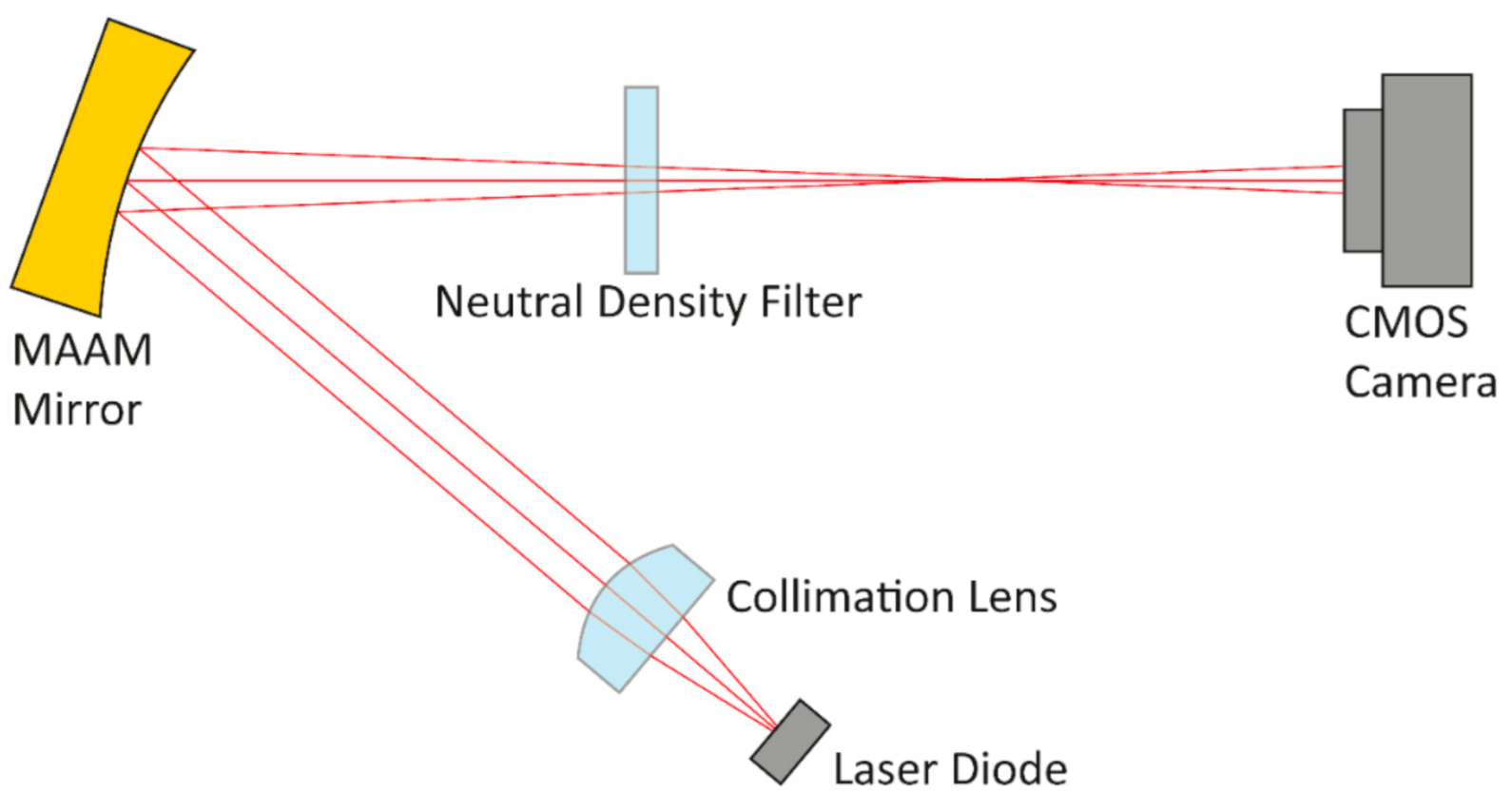
As a characterization setup, an optical system was chosen which could easily be implemented in an optical lab. A highly divergent laser diode beam was first converted into a nearly collimated beam by an aspherical lens, then directed to the MAAM mirror. The fast axis direction of the laser diode, corresponding to the long axis in the elliptical beam profile of the laser, coincided with the long axis of the membrane mirror. From there, the beam was reflected towards a beam profile detection device. The angle of incidence on the mirror was 20°, as close as the mechanical mounts of laser, lens, and mirror would allow. This helped to minimize as much as possible any off-axis aberrations caused by the curved mirror.
Figure 8 schematically shows the characterization setup.
For the transfer into the simulation model, all components which might influence the detected beam profile and for which reliable mechanical and optical design models existed, were imported into an optical simulation tool (FRED [
30]). This was the case for the laser diode housing and the collimation lens. The laser diode source, the lens mount aperture, the MAAM mirror, and the CMOS camera as a beam profile detection device were generated within the optical simulation tool according to the known optical specifications.
Table 3 summarizes the key optical and mechanical specifications.
Because we aimed to develop a general simulation model for laser applications of the MAAM mirror, Gaussian beamlet propagation (GBP) was chosen due to its ability to represent coherent beams in astigmatic beam configurations. GBP was introduced by Arnaud and Kogelnik [
23,
24] as a method to propagate astigmatic Gaussian beamlets through an optical system. It is based on the idea to represent any arbitrary electromagnetic field by a certain number of Gaussian beamlets. With careful choice of beamlet size and sampling, GBP has been demonstrated to provide reliable simulation results for line lasers [
20,
25].
In our setup, the astigmatism in the beam mostly arose from the fast axis divergence of 32° (FWHM) of the laser diode. To determine an appropriate beamlet size and sampling, a practical approach was to observe the simulated irradiance and field phase after free space beam propagation distances which corresponded to the typical overall distances found in the setup. The quality criterion here was to obtain smooth phase profiles in all areas with significant irradiance.
In our case, a sampling of 2048 × 512 beamlets for the fast and slow laser diode beam axis provided reliable simulation results. As an example,
Figure 9 shows the simulated irradiance and fast axis phase profile after 600 mm of free space propagation. The simulated irradiance in
Figure 9a reveals a typical collimated laser diode beam profile of an elliptical shape, the ellipticity originated by the different beam divergence angles (fast axis and slow axis) of the laser diode. Along the fast axis, the irradiance exhibited a modulation, which was caused by diffraction at the collimation lens aperture. The corresponding phase of the coherent field, retrieved from the simulation and depicted in
Figure 9b, showed no phase jumps, which would indicate an insufficient sampling of the coherent field. These intermediate results confirmed that the modeled laser source, consisting of the laser diode and the collimation optics, could serve as the input beam in the optical simulation for the whole system.
Finally, all component positions and orientations were implemented according to the experimental setup, which is described in detail in the next section. With this, the model was complete to simulate the laser beam profile on the detector for variable MAAM mirror radii R in the long axis of the membrane.
2.3. Experimental MAAM Mirror Characterization Setup
The experimental setup was realized according to the parameters described in the previous modelling section. In the setup, the distance between laser diode and MAAM mirror was set to 35 mm, and the distance between the MAAM mirror and CMOS camera chip to 238 mm, respectively. In order to prevent high irradiance-induced saturation effects in the camera, a neutral density filter with an optical density of 3.0 was placed between the MAAM mirror and the camera. The beam profiles changed during the focusing experiments, meaning saturation could still occur. Therefore, the exposure time of the camera was adjusted between 10 ms and 100 ms. Furthermore, the camera gain was set to a value of 0, the gamma correction to a value of 1.
Figure 10a shows the measured beam image in the setup for the MAAM mirror at U = 0 V. The beam showed the expected elliptical shape of a nearly collimated diode laser beam but, in addition, several irradiance variations across the beam profile. These variations were more irregular, compared to the simulation of a freely propagating beam in
Figure 9a. Therefore, it needed to be investigated whether these patterns had their origin in the MAAM mirror or if these patterns were the typical superimposed unintended diffraction patterns of the optical elements, dust particles, and other objects in the beam path [
31,
32]. For clarification, an additional image (
Figure 10b) of the laser beam was taken outside the MAAM mirror setup, where the beam was propagating for just 600 mm in free space. Additionally, for the beam image in
Figure 10b, taken after free space propagation, diffraction effects, similar to the ones in the MAAM mirror setup (
Figure 10a), could be observed. This indicated that the patterns within the beam image observed in our MAAM mirror setup were not dominated by the MAAM mirror and originated mostly from components located before the MAAM mirror in the beam path.
2.4. Evaluation of Simulation and Experimental Data
The evaluation was intended to quantify the effects of the MAAM mirror on the laser beam in the current setup experimentally and by simulations. This was followed by a comparison between experimental data and simulations to validate the simulation model.
Due to the adaptive curvature in the long axis direction of the membrane, the MAAM mirror acted as a variable focusing element in this direction. The perpendicular direction of the beam should have been unaffected by the MAAM focusing device. With radii
R ranging from 6204 mm to 327 mm (see
Table 2), the corresponding focal lengths
f in the fast beam axis varied from 3102 mm to 163.5 mm. When no voltage was applied to the MAAM mirror, the beam width in the fast axis direction was expected to be nearly the collimated beam width. In this state of the mirror, the preset focal length of 3102 mm was very large compared to the distance of 238 mm between the MAAM mirror and camera. Then, with increasing membrane voltages and correspondingly decreasing focal lengths, the focus point in the fast axis moved closer to the camera chip, leading to a decreasing beam width. Once the focal length was in the range of the camera distance, a minimum in the beam width should have been observed. Further decreasing of the focal length set the focus point of the fast axis beam in front of the camera chip, thereby leading to an increasing beam width. Due to the cylindric design of the mirror, the slow axis direction of the beam was expected to remain unchanged in width during the variation of applied voltages, radii, and focal lengths.
As can be seen in
Figure 10a, the measured beam profile did not exhibit a smooth beam profile, but was superimposed by diffractive patterns. These patterns hindered the straightforward extraction of a fast axis beam width out of the measured beam profile. For example, retrieving the irradiance along a horizontal line (pixel row) followed by fitting to a theoretical function led to strong variations in the width parameter of the fit function, depending on the position of the horizontal line. Furthermore, the diffractive patterns changed with varying membrane deformations.
The aforementioned effects required a more robust method to retrieve a fast axis beam width out of the beam profiles. No significant changes in the beam width of the slow axis were observed; therefore, we averaged the irradiances on the camera images of the beam profiles along the pixel columns. This averaging reduced the effect of the superimposed patterns, but still enabled the determination of a measure for the width in the direction perpendicular to the averaging, i.e., the fast beam axis. The resulting curve was then fitted to a Gaussian function of the type:
where
is the column averaged irradiance value at the pixel column position
x,
A is the fitted amplitude,
µ is the fitted center of the profile, and
c is the fitted offset. The fitted width
w could then be used as the required measure for the beam width in the fast axis direction.
As an example,
Figure 11 shows the pixel column averaged beam profile of
Figure 10a, together with the Gaussian function and fitted according to Equation (6). The fitted Gaussian function represents the pixel column averaged irradiance in this example well enough to obtain a reliable measure for the fast axis beam width. Still, an asymmetry in the offsets at +5 mm and −5 mm of the measured averaged irradiance can be observed, which was not accounted for in the fit function. The origin of the asymmetry was not fully examined, but could be caused by stray light in the measurement setup. However, the introduction of a correction term for this offset difference in the fit function did not significantly alter the results for the beam width. Therefore, the fit function of Equation (6) was used for all measured beam profiles.
The evaluation of the results also includes the analysis of the simulation results. Therefore, the same method, averaging the irradiance over camera pixel columns, followed by fitting the resulting profile to a Gaussian function, must be applied to the simulated irradiance distribution. Grid and size of the detector cells in the simulation model were set to the parameters of the used camera; therefore, the results for the beam width w could be directly compared. This gave an indication on the performance of the validation method and the created model.


