
Equilibrium Conformation of a Novel Cable-Driven Snake-Arm Robot under External Loads

Abstract
:1. Introduction
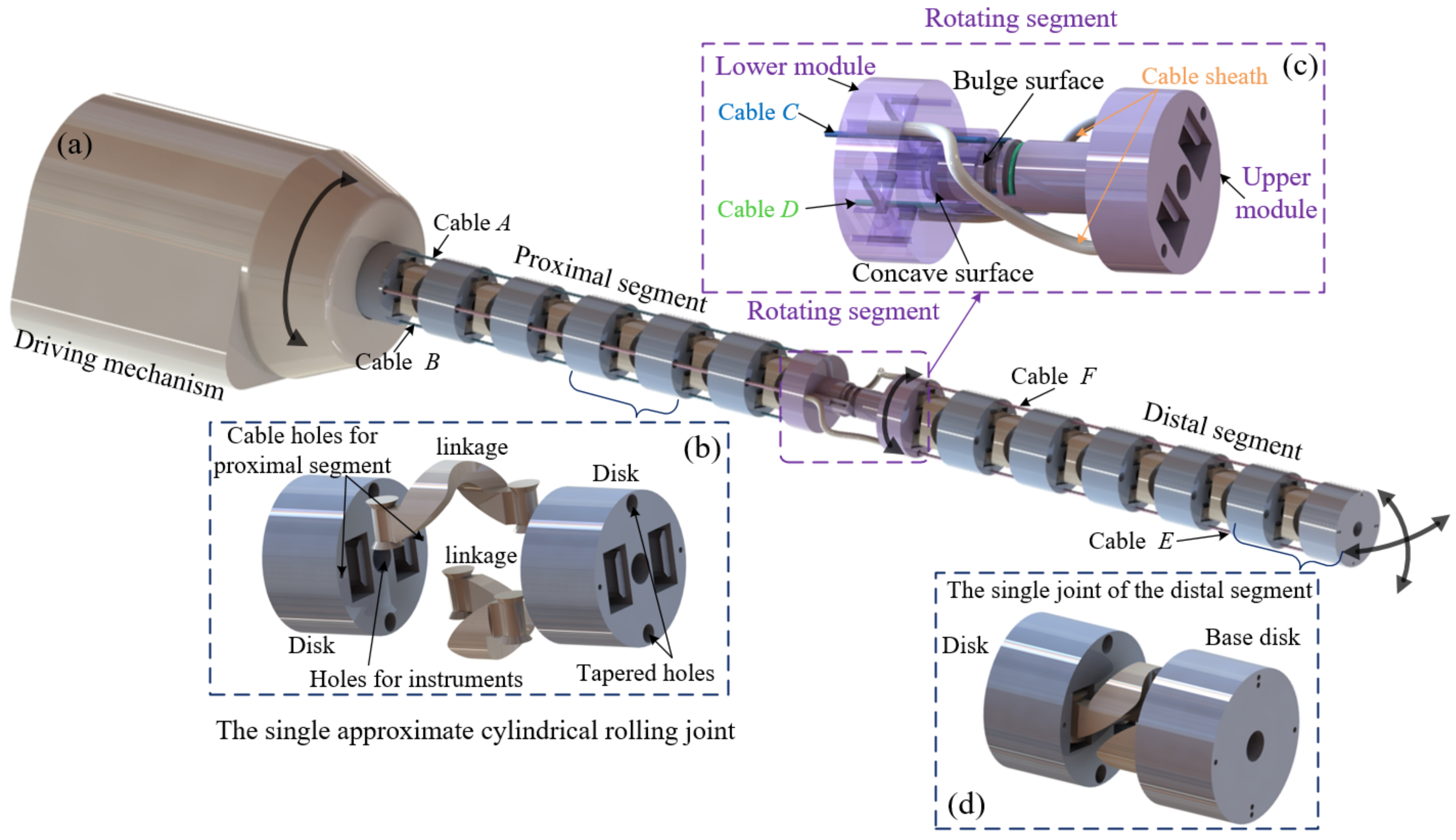
2. Robot Design
2.1. Joint Design
2.2. Manipulator Design
3. Kinematics
3.1. The Mapping between Actuator Space and Task Space
3.2. The Mapping between Actuator Space and Task Space
4. Equilibrium Conformations Analysis under External Loads
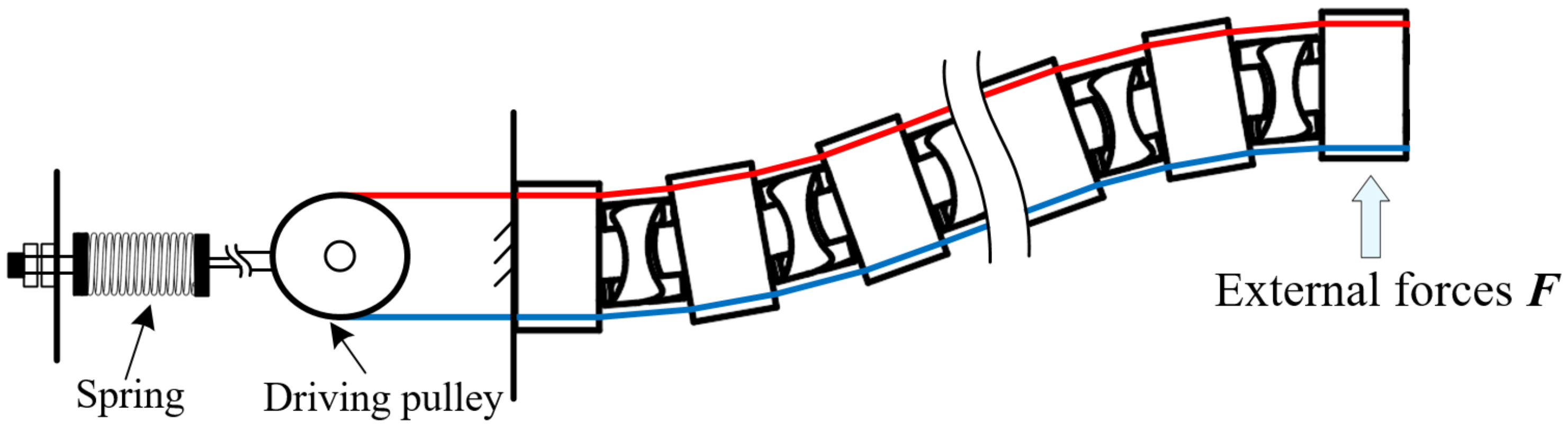
4.1. Static Model
4.2. Solutions
5. Experiments and Discussion
5.1. Robot Prototype
5.2. Free Bending Motion Experiments
5.3. The Load Experiments of the Proximal Segment
5.4. The Load Experiments of the Distal Segment
5.5. Discussion
6. Conclusions
Author Contributions
Funding
Conflicts of Interest
References
- Ji, D.; Kang, T.H.; Shim, S.; Hong, J. Analysis of twist deformation in wire-driven continuum surgical robot. Int. J. Control Autom. Syst. 2020, 18, 10–20. [Google Scholar] [CrossRef]
- Chen, J.; Yang, J.; Qian, F.; Lu, Q.; Guo, Y.; Sun, Z.; Chen, C. A Novel Inchworm-Inspired Soft Robotic Colonoscope Based on a Rubber Bellows. Micromachines 2022, 13, 635. [Google Scholar] [CrossRef] [PubMed]
- Dong, X.; Axinte, D.; Palmer, D.; Cobos, S.; Raffles, M.; Rabani, A.; Kell, J. Development of a slender continuum robotic system for on-wing inspection/repair of gas turbine engines. Robot. Comput. Integr. Manuf. 2017, 44, 218–229. [Google Scholar] [CrossRef] [Green Version]
- Kwon, S.; Kim, J.; Moon, Y.; Kim, K. Hyper-Redundant Manipulator Capable of Adjusting Its Non-Uniform Curvature with Discrete Stiffness Distribution. Appl. Sci. 2022, 12, 482. [Google Scholar] [CrossRef]
- Ito, K.; Maruyama, H. Semi-autonomous serially connected multi-crawler robot for search and rescue. Adv. Robot. 2016, 30, 489–503. [Google Scholar] [CrossRef]
- Liu, B.; Huang, L.; Yin, L.; Zhang, P.; Yi, K. Design and analysis of a tendon-driven snake-arm robot based on spherical magnets. Trans. Can. Soc. Mech. Eng. 2021, 46, 68–76. [Google Scholar] [CrossRef]
- Kim, Y.J.; Cheng, S.; Kim, S.; Iagnemma, K. A stiffness-adjustable hyper redundant manipulator using a variable neutral-line mechanism for minimally invasive surgery. IEEE Trans. Robot. 2013, 30, 382–395. [Google Scholar] [CrossRef] [Green Version]
- Hwang, M.; Kwon, D.S. Strong continuum manipulator for flexible endoscopic surgery. IEEE/ASME Trans. Mechatron. 2019, 24, 2193–2203. [Google Scholar] [CrossRef]
- Kim, J.; Kwon, S.; Kim, K. Novel block mechanism for rolling joints in minimally invasive surgery. Mech. Mach. Theory 2020, 147, 103774. [Google Scholar] [CrossRef]
- Suh, J.W.; Kim, K.Y.; Jeong, J.W.; Lee, J.J. Design considerations for a hyper-redundant pulleyless rolling joint with elastic fixtures. IEEE/ASME Trans. Mechatron. 2015, 20, 2841–2852. [Google Scholar] [CrossRef]
- Bourbonnais, F.; Bigras, P.; Bonev, I.A. Minimum-time trajectory planning and control of a pick-and-place five-bar parallel robot. IEEE/ASME Trans. Mechatron. 2015, 20, 740–749. [Google Scholar] [CrossRef]
- Wang, D.; Wu, J.; Wang, L.; Liu, Y. A postprocessing strategy of a 3-DOF parallel tool head based on velocity control and coarse interpolation. IEEE Trans. Ind. Electron. 2017, 65, 6333–6342. [Google Scholar]
- Black, C.B.; Till, J.; Rucker, D.C. Parallel continuum robots: Modeling, analysis, and actuation-based force sensing. IEEE Trans. Robot. 2017, 34, 29–47. [Google Scholar] [CrossRef]
- Shin, W.H.; Kwon, D.S. Surgical robot system for single-port surgery with novel joint mechanism. IEEE Trans. Biomed. Eng. 2013, 60, 937–944. [Google Scholar] [CrossRef]
- Zhang, L.; Wang, S.; Li, J.; Wang, X.; He, C.; Qu, J. A novel reconfigurable unit for high dexterous surgical instrument. In Advances in Reconfigurable Mechanisms and Robots I; Springer: London, UK, 2012; pp. 433–442. [Google Scholar]
- Gao, G.H.; Wang, P.; Wang, H. Follow-the-leader motion strategy for multi-section continuum robots based on differential evolution algorithm. Industrial Robot: Int. J. Robot. Res. Appl. 2021, 4, 589–601. [Google Scholar] [CrossRef]
- Huang, L.; Yin, L.; Liu, B.; Yang, Y. Design and error evaluation of planar 2DOF remote center of motion mechanisms with cable transmissions. J. Mech. Des. 2021, 143, 013301. [Google Scholar] [CrossRef]
- Wu, Z.; Li, Q.; Zhao, J.; Gao, J.; Xu, K. Design of a modular continuum-articulated laparoscopic robotic tool with decoupled kinematics. IEEE Robot. Autom. Lett. 2019, 4, 3545–3552. [Google Scholar] [CrossRef]
- Phee, S.J.; Kencana, A.P.; Huynh, V.A.; Sun, Z.L.; Low, S.C.; Yang, K.; Lomanto, D.; Ho, K.Y. Design of a master and slave transluminal endoscopic robot for natural orifice transluminal endoscopic surgery. Proc. Inst. Mech. Eng. Part C J. Mech. Eng. Sci. 2010, 224, 1495–1503. [Google Scholar] [CrossRef]
- Ye, T.; Wang, Y.; Xu, S.; Wang, Y.; Li, J. Modeling and motion control of an octopus-like flexible manipulator actuated by shape memory alloy wires. J. Intell. Mater. Syst. Struct. 2022, 33, 3–16. [Google Scholar] [CrossRef]
- Schaffner, M.; Faber, J.A.; Pianegonda, L.; Rühs, P.A.; Coulter, F.; Studart, A.R. 3D printing of robotic soft actuators with programmable bioinspired architectures. Nat. Commun. 2018, 9, 878. [Google Scholar] [CrossRef]
- Endo, N.; Kizaki, Y.; Kamamichi, N. Flexible pneumatic bending actuator for a robotic tongue. J. Robot. Mechatron. 2020, 32, 894–902. [Google Scholar] [CrossRef]
- Takikawa, K.; Miyazaki, R.; Kanno, T.; Endo, G.; Kawashima, K. Pneumatically Driven Multi-DOF Surgical Forceps Manipulator with a Bending Joint Mechanism Using Elastic Bodies. J. Robot. Mechatron. 2016, 28, 559–567. [Google Scholar] [CrossRef]
- Burgner-Kahrs, J.; Rucker, D.C.; Choset, H. Continuum robots for medical applications: A survey. IEEE Trans. Robot. 2015, 31, 1261–1280. [Google Scholar] [CrossRef]
- Li, C.; Rahn, C.D. Design of continuous backbone, cable-driven robots. J. Mech. Des. 2002, 124, 265–271. [Google Scholar] [CrossRef]
- Alqumsan, A.A.; Khoo, S.; Norton, M. Robust control of continuum robots using Cosserat rod theory. Mech. Mach. Theory 2019, 131, 48–61. [Google Scholar] [CrossRef]
- Xu, K.; Simaan, N. Analytic formulation for kinematics, statics, and shape restoration of multi-backbone continuum robots via elliptic integrals. J. Mech. Robot. 2010, 2, 011006. [Google Scholar] [CrossRef] [Green Version]
- Yang, C.; Geng, S.; Walker, I.; Branson, D.T.; Liu, J.; Dai, J.S.; Kang, R. Geometric constraint-based modeling and analysis of a novel continuum robot with Shape Memory Alloy initiated variable stiffness. Int. J. Robot. Res. 2020, 39, 1620–1634. [Google Scholar] [CrossRef]
- Venkiteswaran, V.K.; Sikorski, J.; Misra, S. Shape and contact force estimation of continuum manipulators using pseudo rigid body models. Mech. Mach. Theory 2019, 139, 34–45. [Google Scholar] [CrossRef]
- Huang, L.; Liu, B.; Yin, L.; Zeng, P.; Yang, Y. Design and Validation of a Novel Cable-Driven Hyper-Redundant Robot Based on Decoupled Joints. J. Robot. 2021, 2021, 5124816. [Google Scholar] [CrossRef]
- Li, Z.; Du, R.; Yu, H.; Ren, H. Statics modeling of an underactuated wire-driven flexible robotic arm. In Proceedings of the 5th IEEE RAS/EMBS International Conference on Biomedical Robotics and Biomechatronics, Sao Paulo, Brazil, 12–15 August 2014; IEEE: Piscataway, NJ, USA, 2014; pp. 326–331. [Google Scholar]
- Wang, H.; Wang, X.; Yang, W.; Du, Z.; Yan, Z. Construction of controller model of notch continuum manipulator for laryngeal surgery based on hybrid method. IEEE/ASME Trans. Mechatron. 2020, 26, 1022–1032. [Google Scholar] [CrossRef]
- Kato, T.; Okumura, I.; Kose, H.; Takagi, K.; Hata, N. Tendon-driven continuum robot for neuroendoscopy: Validation of extended kinematic mapping for hysteresis operation. Int. J. Comput. Assist. Radiol. Surg. 2016, 11, 589–602. [Google Scholar] [CrossRef] [PubMed] [Green Version]
- Chen, Z.; Liu, Z.; Han, X. Model Analysis of Robotic Soft Arms including External Force Effects. Micromachines 2022, 13, 350. [Google Scholar] [CrossRef] [PubMed]
- Kim, Y.J.; Kim, J.I.; Jang, W. Quaternion joint: Dexterous 3-DOF joint representing quaternion motion for high-speed safe interaction. In Proceedings of the 2018 IEEE/RSJ International Conference on Intelligent Robots and Systems (IROS), Madrid, Spain, 1–5 October 2018; IEEE: Piscataway, NJ, USA, 2018; pp. 935–942. [Google Scholar]
- Huang, L.; Zeng, P.; Yin, L.; Liu, B.; Yang, Y.; Huang, J. Design and kinematic analysis of a rigid-origami-based underwater sampler with deploying-encircling motion. Mech. Mach. Theory 2022, 174, 104886. [Google Scholar] [CrossRef]
- Lebedev, P.A. Vector method for the synthesis of mechanisms. Mech. Mach. Theory 2003, 38, 265–276. [Google Scholar] [CrossRef]
- Sun, X.; Li, R.; Xun, Z.; Yao, Y.A. A new Bricard-like mechanism with anti-parallelogram units. Mech. Mach. Theory 2020, 147, 103753. [Google Scholar] [CrossRef]
- Miao, Z.; Yao, Y.; Kong, X. A rolling 3-UPU parallel mechanism. Front. Mech. Eng. 2013, 8, 340–349. [Google Scholar] [CrossRef]
- Yuan, H.; Li, Z. Workspace analysis of cable-driven continuum manipulators based on static model. Robot. Comput. Integr. Manuf. 2018, 49, 240–252. [Google Scholar] [CrossRef]
- Xu, W.; Liu, T.; Li, Y. Kinematics, dynamics, and control of a cable-driven hyper-redundant manipulator. IEEE/ASME Trans. Mechatron. 2018, 23, 1693–1704. [Google Scholar] [CrossRef]
- Hu, B.; Zhou, C.; Wang, H.; Chen, S. Nonlinear tribo-dynamic model and experimental verification of a spur gear drive under loss-of-lubrication condition. Mech. Syst. Signal Processing 2021, 153, 107509. [Google Scholar] [CrossRef]
- Yang, C.; Kang, R.; Branson, D.T.; Chen, L.; Dai, J.S. Kinematics and statics of eccentric soft bending actuators with external payloads. Mech. Mach. Theory 2019, 139, 526–541. [Google Scholar] [CrossRef]
- Dalvand, M.M.; Nahavandi, S.; Howe, R.D. An analytical loading model for n-tendon continuum robots. IEEE Trans. Robot. 2018, 34, 1215–1225. [Google Scholar] [CrossRef]
- Zheng, Y.; Wu, B.; Chen, Y.; Zeng, L.; Gu, G.; Zhu, X.; Xu, K. Design and validation of cable-driven hyper-redundant manipulator with a closed-loop puller-follower controller. Mechatronics 2021, 78, 102605. [Google Scholar] [CrossRef]


| Symbols | Descriptions | Values |
|---|---|---|
| hc | The initial distance between the major axes of adjacent ellipses | 15 mm |
| r | Cable distribution circle radius | 9 mm |
| R | Cylindrical rolling radius | 10.5 mm |
| wc | The distance between the two focuses of the ellipse | 10 mm |
| ψ | The angle of joint bending | [−π/9, π/9] |
| h0 | The distance between the circle center and the upper surface of the lower disk | 3 mm |
| h1 | The distance between the major axis and the upper surface of the lower disk | 2.0 mm |
| h2 | The thickness of a single disk | 11.5 mm |
| h3 | The initial height of the single joint | 11.0 mm |
| h4 | The distance between the circle center and the upper surface of the lower disk | 5 mm |
Publisher’s Note: MDPI stays neutral with regard to jurisdictional claims in published maps and institutional affiliations. |
© 2022 by the authors. Licensee MDPI, Basel, Switzerland. This article is an open access article distributed under the terms and conditions of the Creative Commons Attribution (CC BY) license (https://creativecommons.org/licenses/by/4.0/).
Share and Cite
Huang, L.; Liu, B.; Zhang, L.; Yin, L. Equilibrium Conformation of a Novel Cable-Driven Snake-Arm Robot under External Loads. Micromachines 2022, 13, 1149. https://doi.org/10.3390/mi13071149
Huang L, Liu B, Zhang L, Yin L. Equilibrium Conformation of a Novel Cable-Driven Snake-Arm Robot under External Loads. Micromachines. 2022; 13(7):1149. https://doi.org/10.3390/mi13071149
Chicago/Turabian StyleHuang, Long, Bei Liu, Leiyu Zhang, and Lairong Yin. 2022. "Equilibrium Conformation of a Novel Cable-Driven Snake-Arm Robot under External Loads" Micromachines 13, no. 7: 1149. https://doi.org/10.3390/mi13071149