


Development of Robust Steel Alloys for Laser-Directed Energy Deposition via Analysis of Mechanical Property Sensitivities †
 , , , ,
Abstract
:1. Introduction
2. Materials and Methods
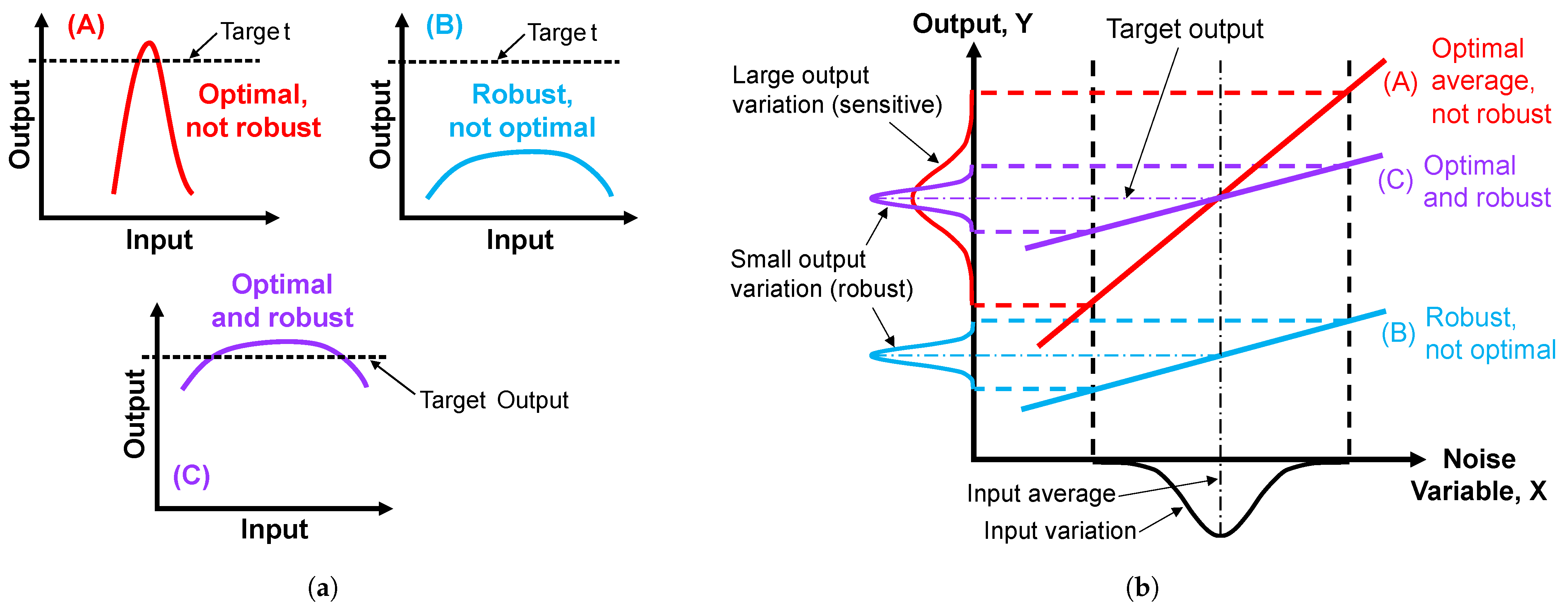
2.1. Quantifying Robustness

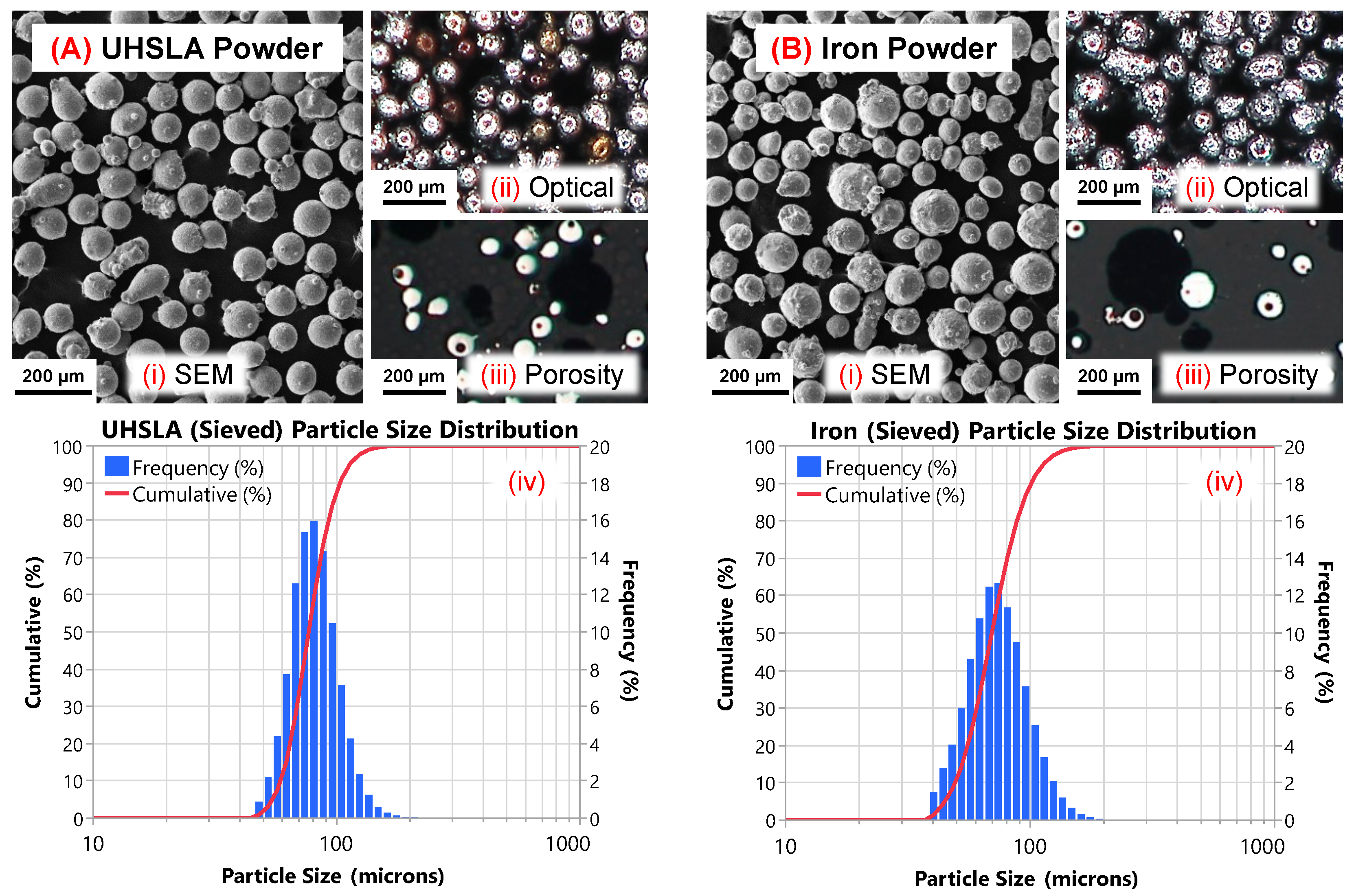
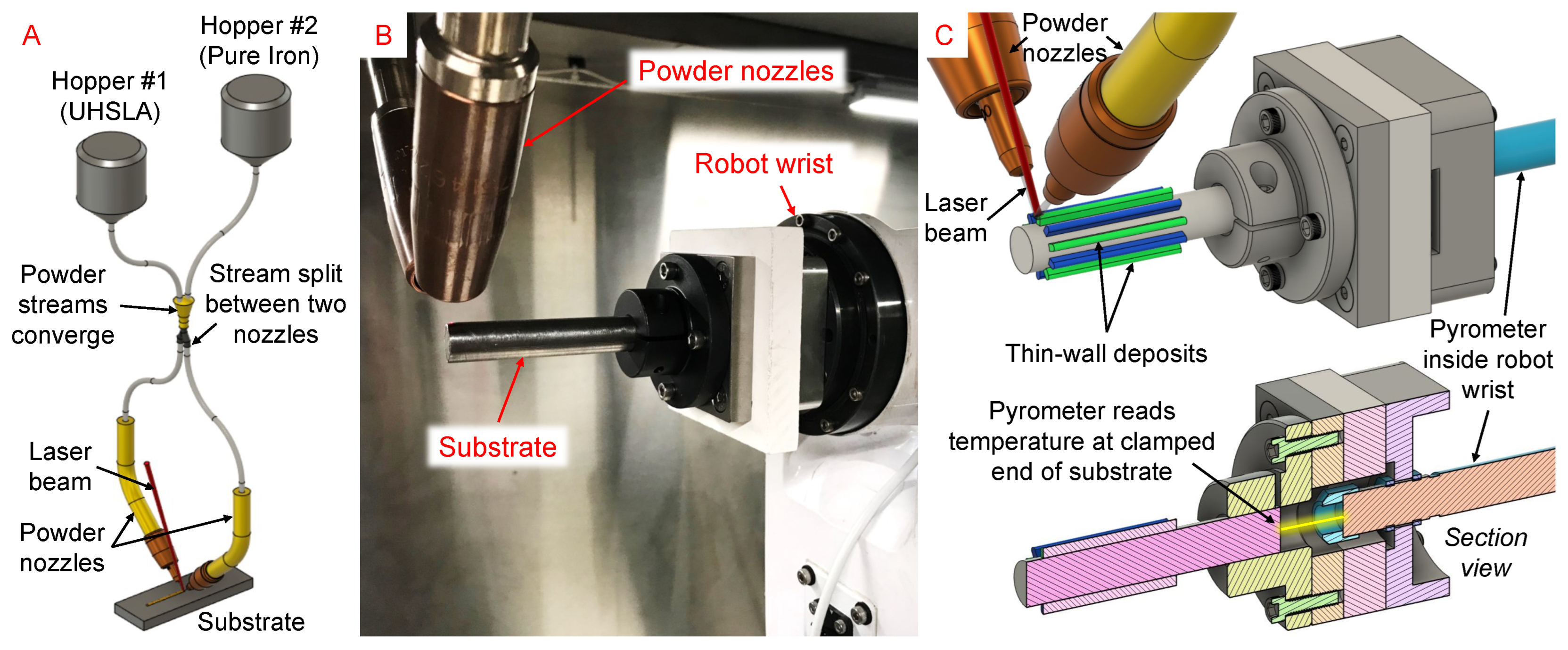
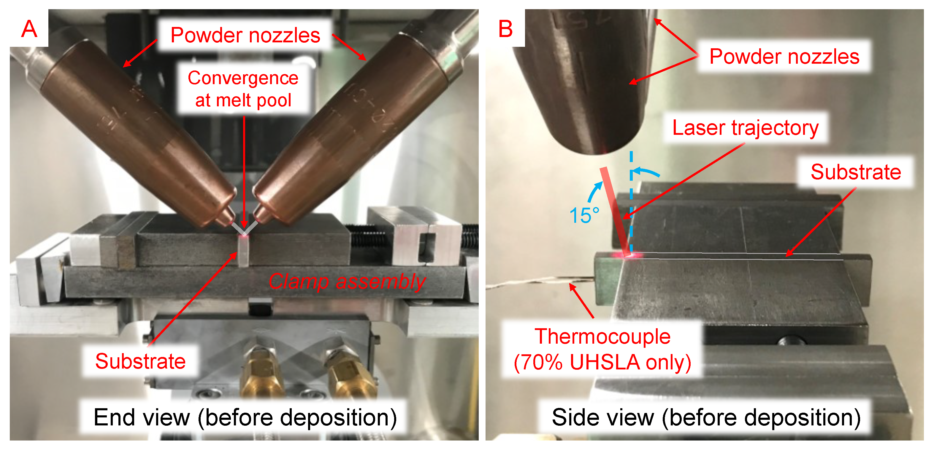
2.2. Materials and Equipment

| Element | Fe | Cr | Ni | Si | Mo | Mn | C | V | Cu |
|---|---|---|---|---|---|---|---|---|---|
| UHSLA powder | Balance | 2.6 | 1.0 | 1.0 | 0.86 | 0.6 | 0.28 | 0.15 | <0.2 |
| Iron powder | 99.89% min | 0.0295 | 0.008 | 0.0001 | 0.001 | 0.012 | 0.0075 | - | 0.0095 |
| Element | O | P | S | Al | Ti | P+Sn+As+Sb | H | N | W |
| UHSLA powder | 0.03 | 0.009 | 0.005 | 0.004 | <0.006 | <0.035 | 6 ppm | - | - |
| Iron powder | 431 ppm | - | - | - | 0.0038 | - | - | 63 ppm | 0.042 |
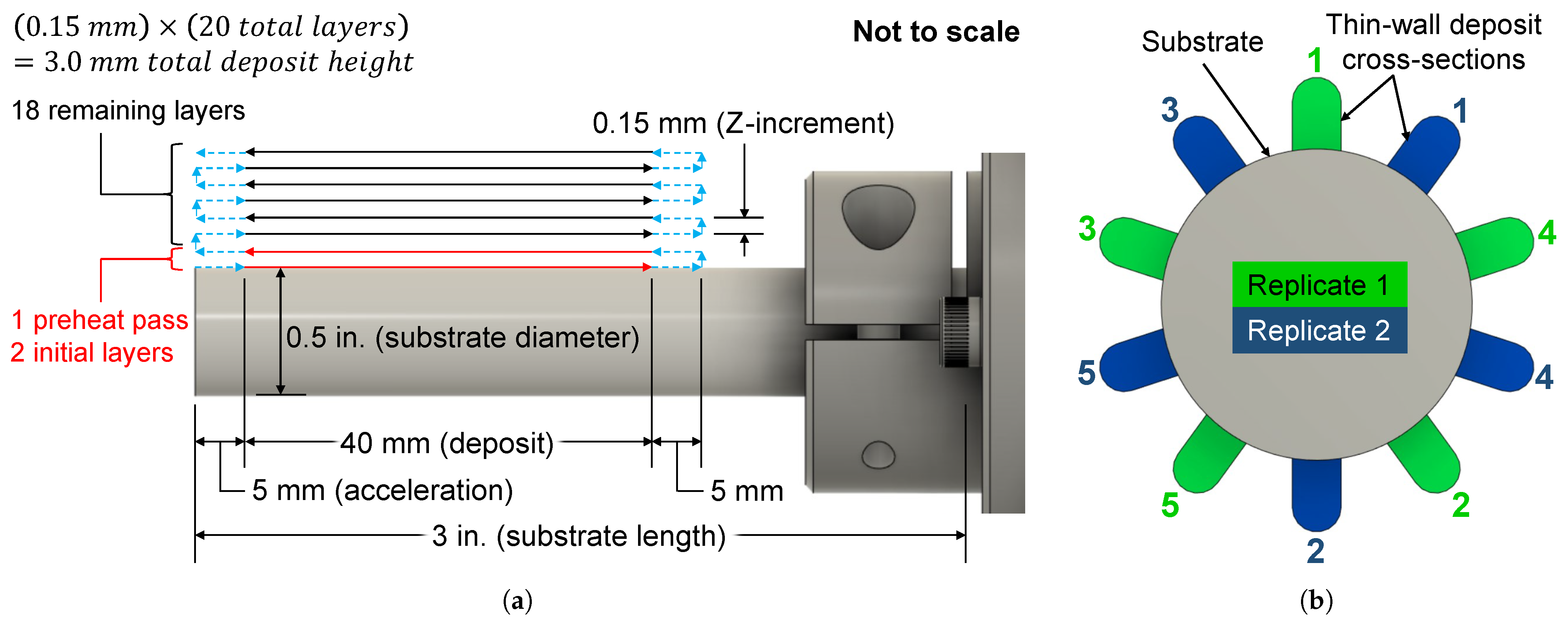
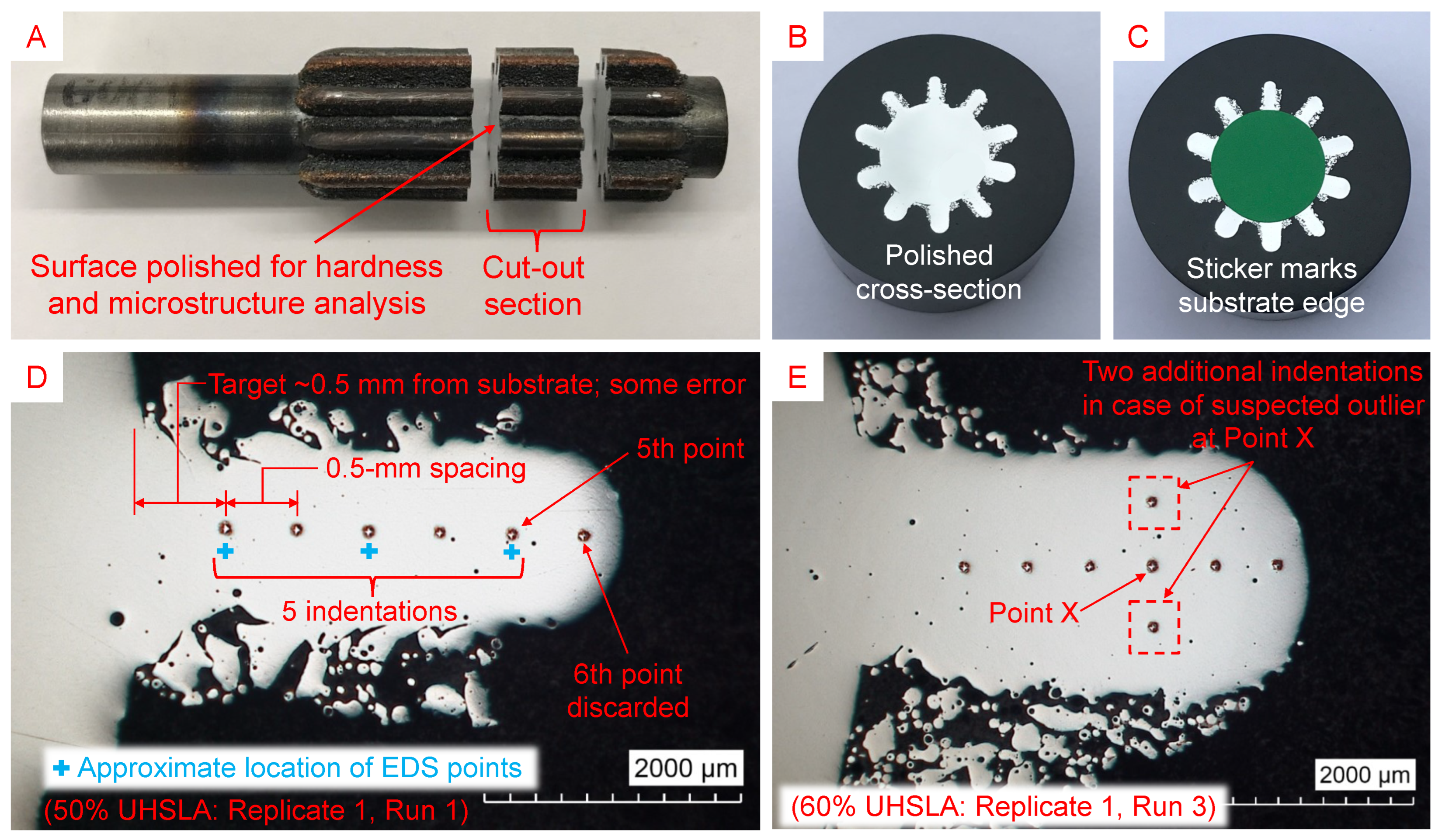
2.3. Experiment #1: Hardness Sensitivity
| Replicate 1 | |||||
|---|---|---|---|---|---|
| Run | 1 | 2 | 3 | 4 | 5 |
| Laser Power (W) | 650 | 1050 | 850 | 1050 | 650 |
| Interlayer Delay (s) | 11 | 1 | 6 | 11 | 1 |
| Replicate 2 | |||||
| Run | 1 | 2 | 3 | 4 | 5 |
| Laser Power (W) | 650 | 1050 | 650 | 850 | 1050 |
| Interlayer Delay (s) | 1 | 11 | 11 | 6 | 1 |
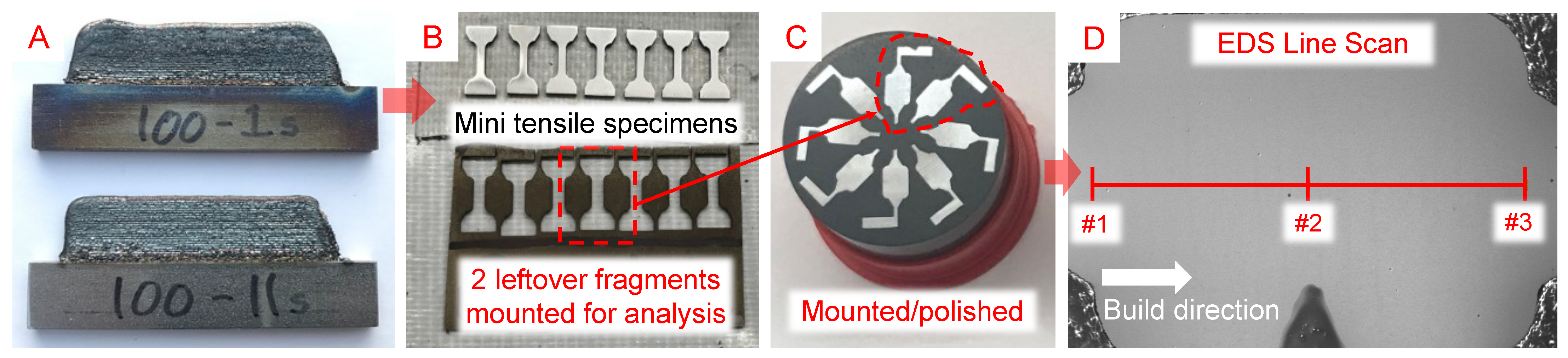
2.4. Experiment #2: Tensile Property Sensitivity

3. Results and Discussion
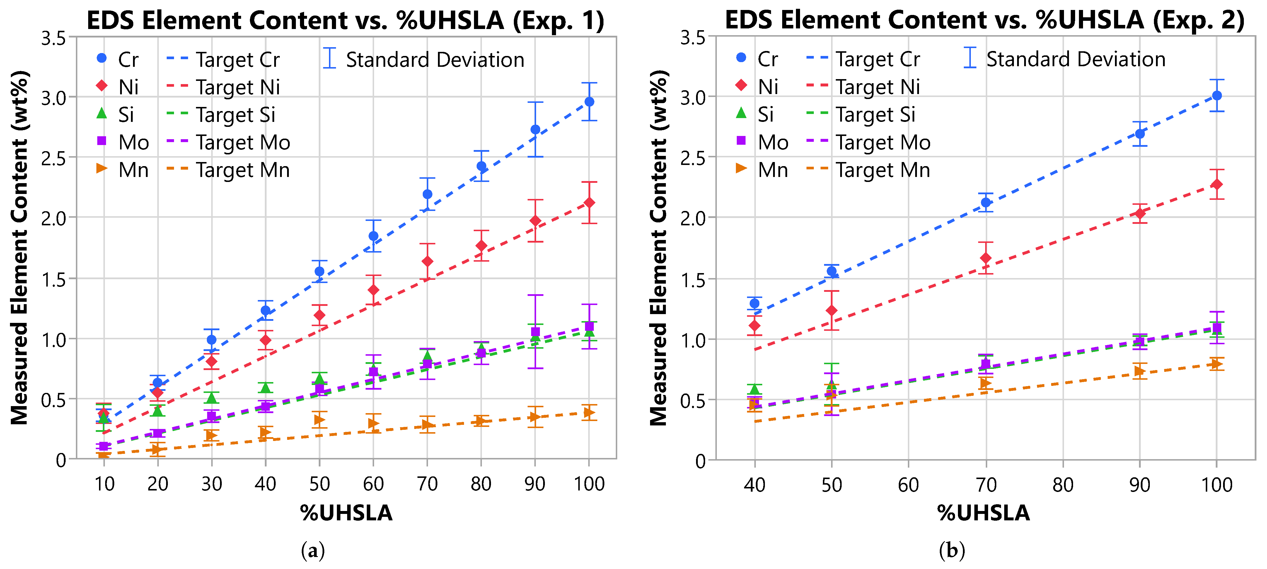
3.1. EDS Analysis
3.2. Temperature History

3.3. Vickers Hardness

| %UHSLA | 10 | 20 | 30 | 40 | 50 | 60 | 70 | 80 | 90 | 100 |
|---|---|---|---|---|---|---|---|---|---|---|
| Mean Hardness (HV) | 127.7 | 168.2 | 229.0 | 272.5 | 332.1 | 375.5 | 417.8 | 440.6 | 469.7 | 487.7 |
| Mean Hardness (HRC) * | - | - | - | 26 | 34 | 38 | 42 | 44 | 47 | 48 |
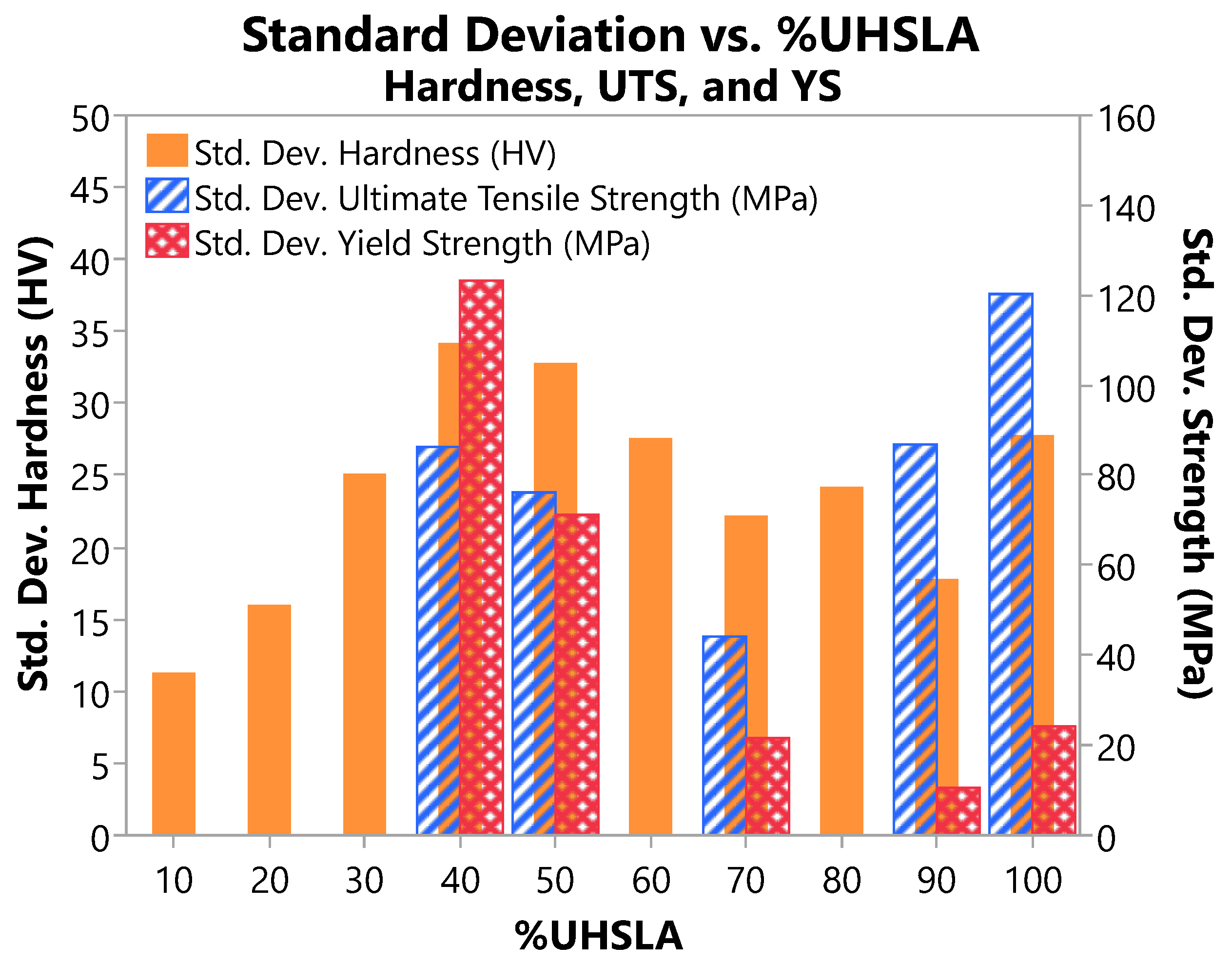
| Std. Dev. Hardness (HV) | 11.3 | 16.0 | 25.1 | 34.2 | 32.8 | 27.6 | 22.2 | 24.2 | 17.8 | 27.8 |
| CV Hardness (%) | 8.9 | 9.5 | 11.0 | 12.5 | 9.9 | 7.4 | 5.3 | 5.5 | 3.8 | 5.7 |

3.4. Hardness Sensitivity
| %UHSLA | 10 | 20 | 30 | 40 | 50 | 60 | 70 | 80 | 90 | 100 |
|---|---|---|---|---|---|---|---|---|---|---|
| R2—Replicate 1&2 | 0.15 | 0.40 | 0.50 | 0.54 | 0.65 | 0.54 | 0.21 | 0.15 | 0.16 | 0.20 |
| R2—Replicate 1 | 0.30 | 0.49 | 0.50 | 0.70 | 0.75 | 0.55 | 0.21 | 0.25 | 0.38 | 0.35 |
| R2—Replicate 2 | 0.08 | 0.41 | 0.57 | 0.46 | 0.64 | 0.61 | 0.38 | 0.45 | 0.47 | 0.27 |
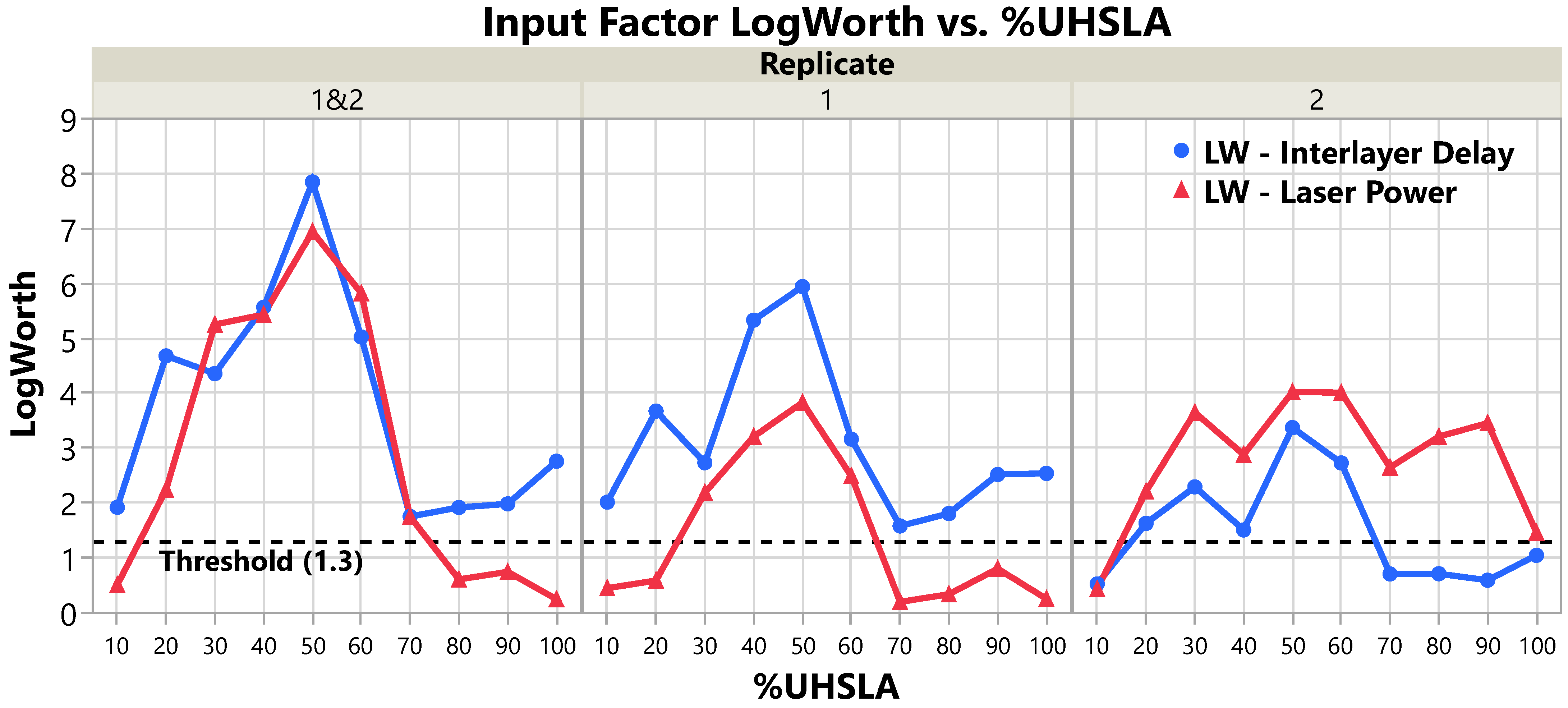
| %UHSLA | 10 | 20 | 30 | 40 | 50 | 60 | 70 | 80 | 90 | 100 | |
|---|---|---|---|---|---|---|---|---|---|---|---|
| Replicate 1&2 | 0.51 | 2.24 | 5.25 | 5.43 | 6.94 | 5.02 | 1.75 | 0.61 | 0.74 | 0.25 | |
| 1.92 | 4.68 | 4.36 | 5.57 | 7.85 | 5.82 | 1.75 | 1.92 | 1.98 | 2.76 | ||
| Replicate 1 | 0.45 | 0.59 | 2.19 | 3.21 | 3.83 | 2.49 | 0.20 | 0.34 | 0.80 | 0.25 | |
| 2.01 | 3.67 | 2.73 | 5.33 | 5.94 | 3.16 | 1.58 | 1.81 | 2.52 | 2.54 | ||
| Replicate 2 | 0.43 | 2.21 | 3.65 | 2.88 | 4.02 | 4.01 | 2.65 | 3.21 | 3.45 | 1.46 | |
| 0.52 | 1.63 | 2.29 | 1.51 | 3.37 | 2.73 | 0.71 | 0.71 | 0.59 | 1.05 |
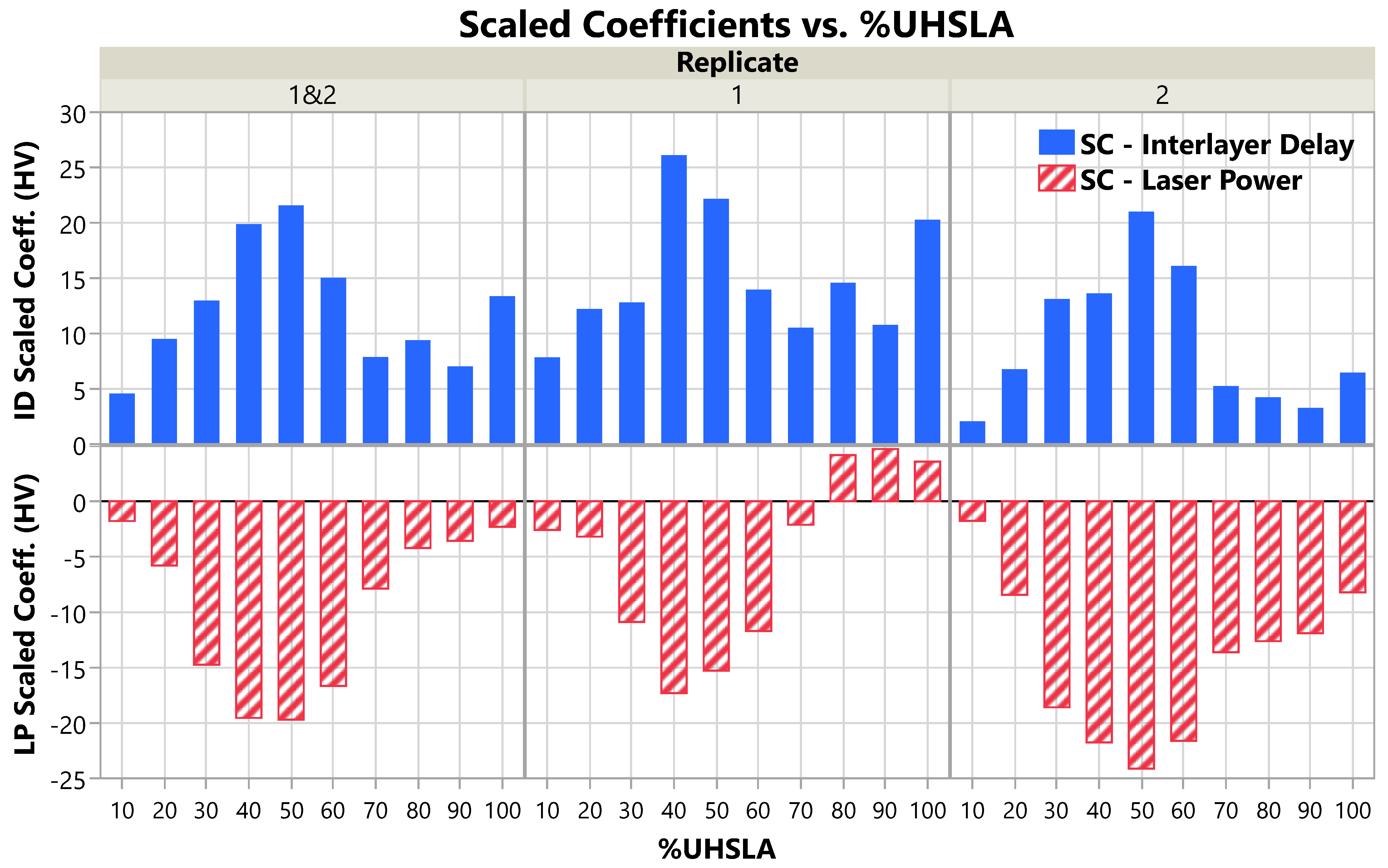
| %UHSLA | 10 | 20 | 30 | 40 | 50 | 60 | 70 | 80 | 90 | 100 | |
|---|---|---|---|---|---|---|---|---|---|---|---|
| Replicate 1&2 | −1.8 | −5.8 | −14.7 | −19.5 | −19.7 | −16.7 | −7.9 | −4.2 | −3.6 | −2.3 | |
| 4.6 | 9.5 | 13.0 | 19.9 | 21.6 | 15.0 | 7.9 | 9.4 | 7.0 | 13.4 | ||
| Replicate 1 | −2.6 | −3.2 | −10.9 | −17.3 | −15.3 | −11.7 | −2.1 | 4.2 | 4.7 | 3.6 | |
| 7.9 | 12.2 | 12.8 | 26.1 | 22.2 | 14.0 | 10.5 | 14.6 | 10.8 | 20.3 | ||
| Replicate 2 | −1.8 | −8.4 | −18.6 | −21.8 | −24.1 | −21.6 | −13.6 | −12.6 | −11.9 | −8.2 | |
| 2.1 | 6.8 | 13.1 | 13.6 | 21.0 | 16.1 | 5.2 | 4.2 | 3.3 | 6.5 |
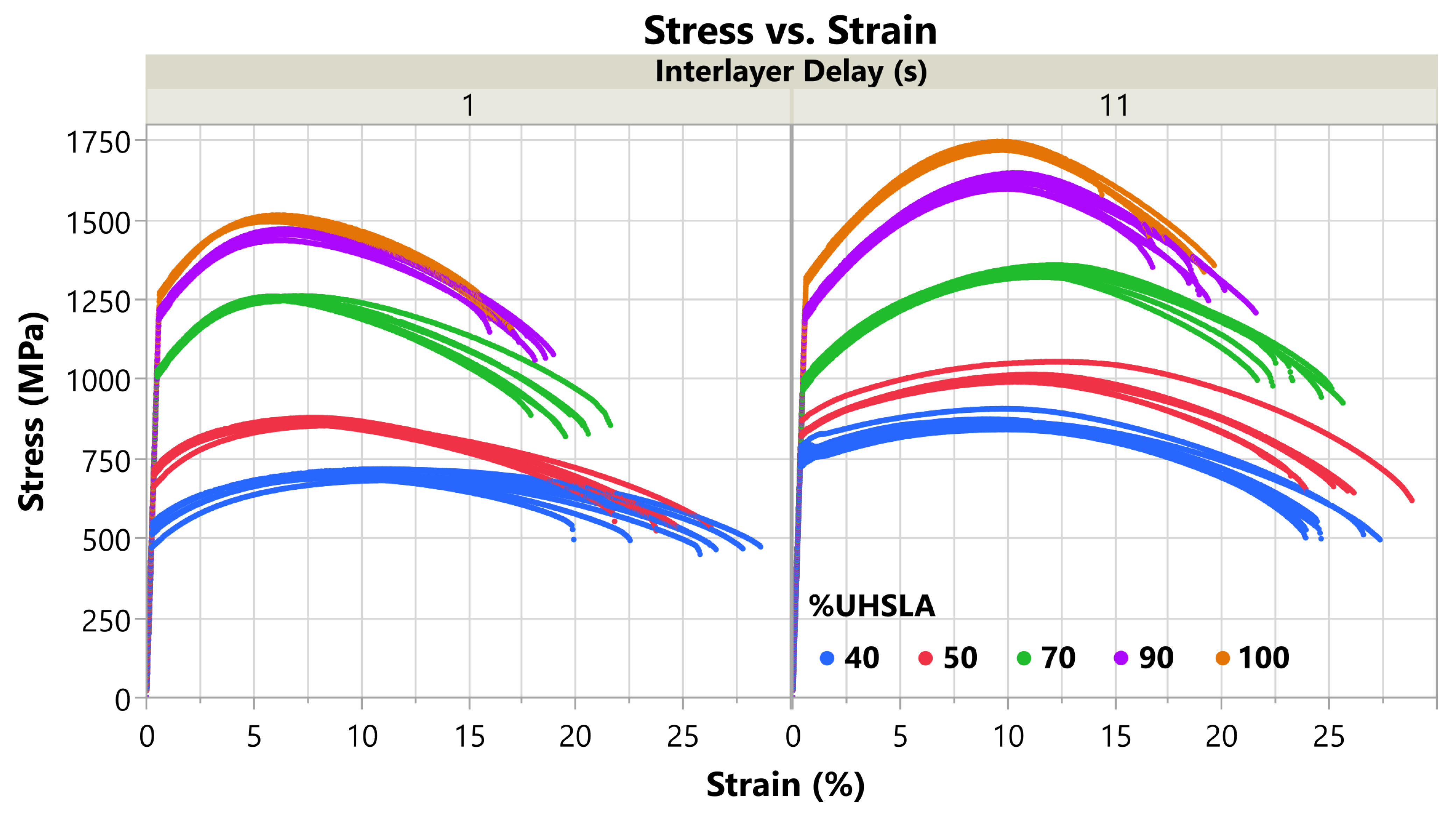
3.5. Tensile Properties
| Data Included | %UHSLA | UTS (MPa) | YS (MPa) | %El | Modulus of Toughness (J/m3) |
|---|---|---|---|---|---|
| All Data | 40 | 784.8 ± 86.3 * | 640.2 ± 123.3 * | 25.2 ± 2.3 | 1.78 × 10⁸ ± 0.24 × 10⁸ |
| 50 | 939.5 ± 76.2 * | 765.9 ± 71.2 * | 24.8 ± 1.8 | 2.10 × 10⁸ ± 0.30 × 10⁸ | |
| 70 | 1296.3 ± 44.2 * | 997.3 ± 21.6 * | 21.7 ± 2.3 | 2.54 × 10⁸ ± 0.36 × 10⁸ | |
| 90 | 1547.6 ± 86.9 * | 1202.2 ± 10.6 * | 18.4 ± 1.5 | 2.58 × 10⁸ ± 0.29 × 10⁸ | |
| 100 | 1632.3 ± 120.3 * | 1288.1 ± 24.2 * | 16.9 ± 1.4 | 2.52 × 10⁸ ± 0.32 × 10⁸ | |
| Interlayer Delay 1 s | 40 | 703.3 ± 14.1 | 523.5 ± 26.6 | 25.3 ± 3.1 | 1.62 × 10⁸ ± 0.21 × 10⁸ |
| 50 | 868.3 ± 10.1 | 700.0 ± 20.1 | 24.1 ± 1.5 | 1.86 × 10⁸ ± 0.11 × 10⁸ | |
| 70 | 1254.6 ± 5.5 | 1016.4 ± 5.6 | 19.8 ± 1.2 | 2.22 × 10⁸ ± 0.14 × 10⁸ | |
| 90 | 1458.8 ± 12.6 | 1200.3 ± 11.3 | 17.8 ± 1.0 | 2.36 × 10⁸ ± 0.13 × 10⁸ | |
| 100 | 1507.0 ± 7.8 | 1264.2 ± 7.9 | 16.3 ± 0.4 | 2.26 × 10⁸ ± 0.54 × 10⁸ | |
| Interlayer Delay 11 s | 40 | 866.3 ± 20.8 | 756.9 ± 21.7 | 25.0 ± 1.4 | 1.95 × 10⁸ ± 0.12 × 10⁸ |
| 50 | 1010.6 ± 23.0 | 831.7 ± 18.4 | 25.5 ± 2.0 | 2.33 × 10⁸ ± 0.22 × 10⁸ | |
| 70 | 1338.0 ± 11.7 | 978.3 ± 11.3 | 23.6 ± 1.5 | 2.85 × 10⁸ ± 0.18 × 10⁸ | |
| 90 | 1623.7 ± 18.2 | 1203.9 ± 10.5 | 18.9 ± 1.7 | 2.77 × 10⁸ ± 0.24 × 10⁸ | |
| 100 | 1736.7 ± 10.4 | 1308.0 ± 8.4 | 17.4 ± 1.8 | 2.73 × 10⁸ ± 0.28 × 10⁸ |
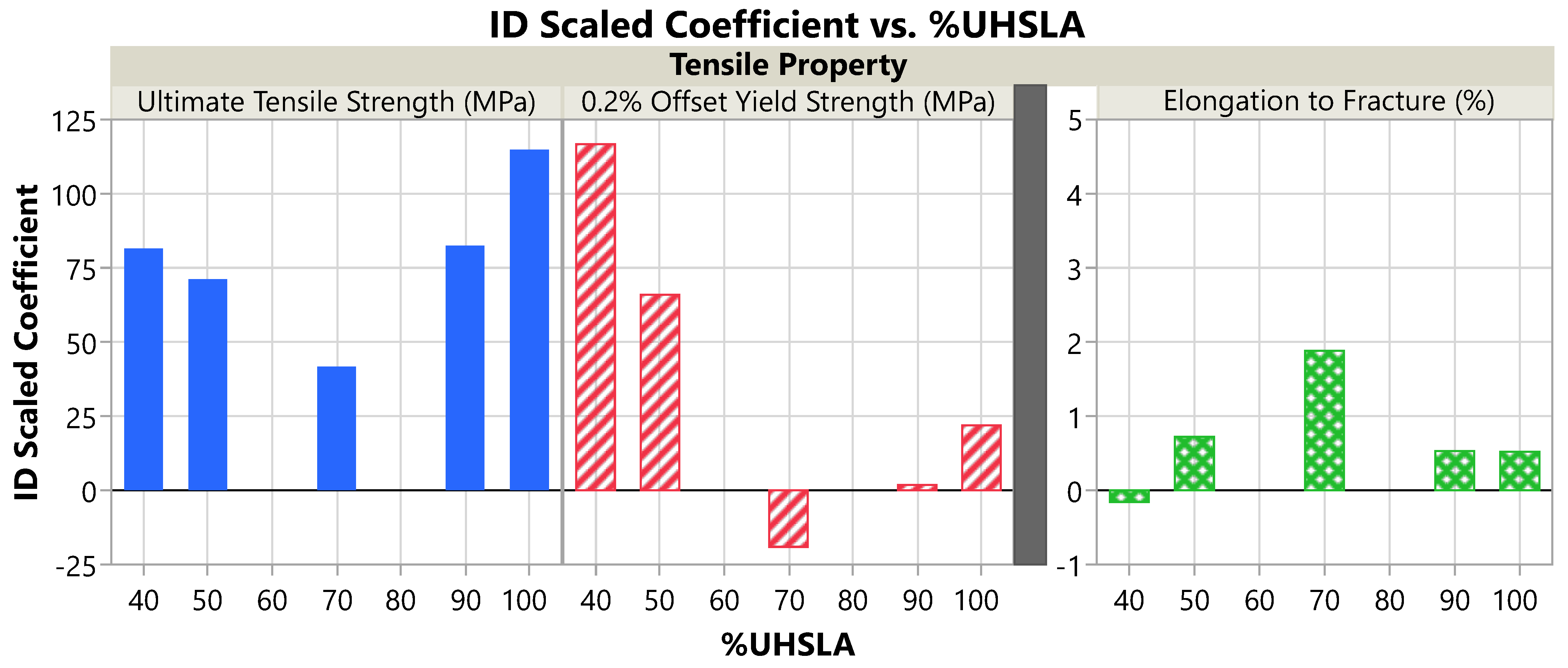
3.6. Tensile Property Sensitivity

| %UHSLA | UTS- R2 | YS- R2 | %El- R2 | UTS- | YS- | %El- | UTS- | YS- | %El- |
|---|---|---|---|---|---|---|---|---|---|
| 40 | 0.96 | 0.96 | 0.01 | 9.08 | 9.32 | 0.10 | 81.49 | 116.70 | −0.16 |
| 50 | 0.95 | 0.93 | 0.17 | 7.13 | 6.48 | 0.74 | 71.15 | 65.88 | 0.72 |
| 70 | 0.96 | 0.84 | 0.69 | 9.06 | 5.43 | 3.62 | 41.71 | −19.09 | 1.88 |
| 90 | 0.97 | 0.03 | 0.14 | 8.95 | 0.24 | 0.67 | 82.44 | 1.76 | 0.53 |
| 100 | 1.00 | 0.90 | 0.15 | 10.79 | 5.00 | 0.61 | 114.83 | 21.90 | 0.52 |
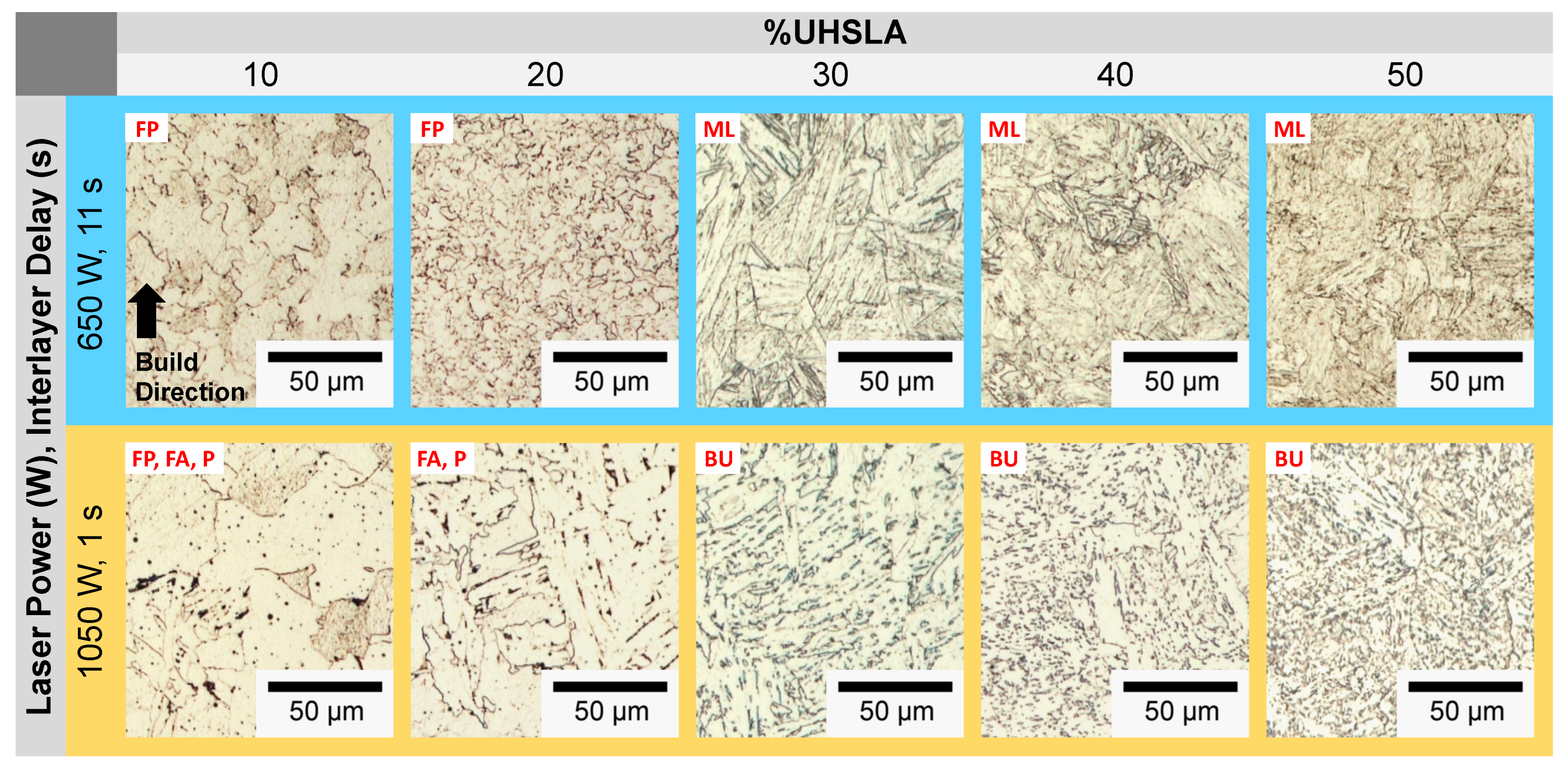
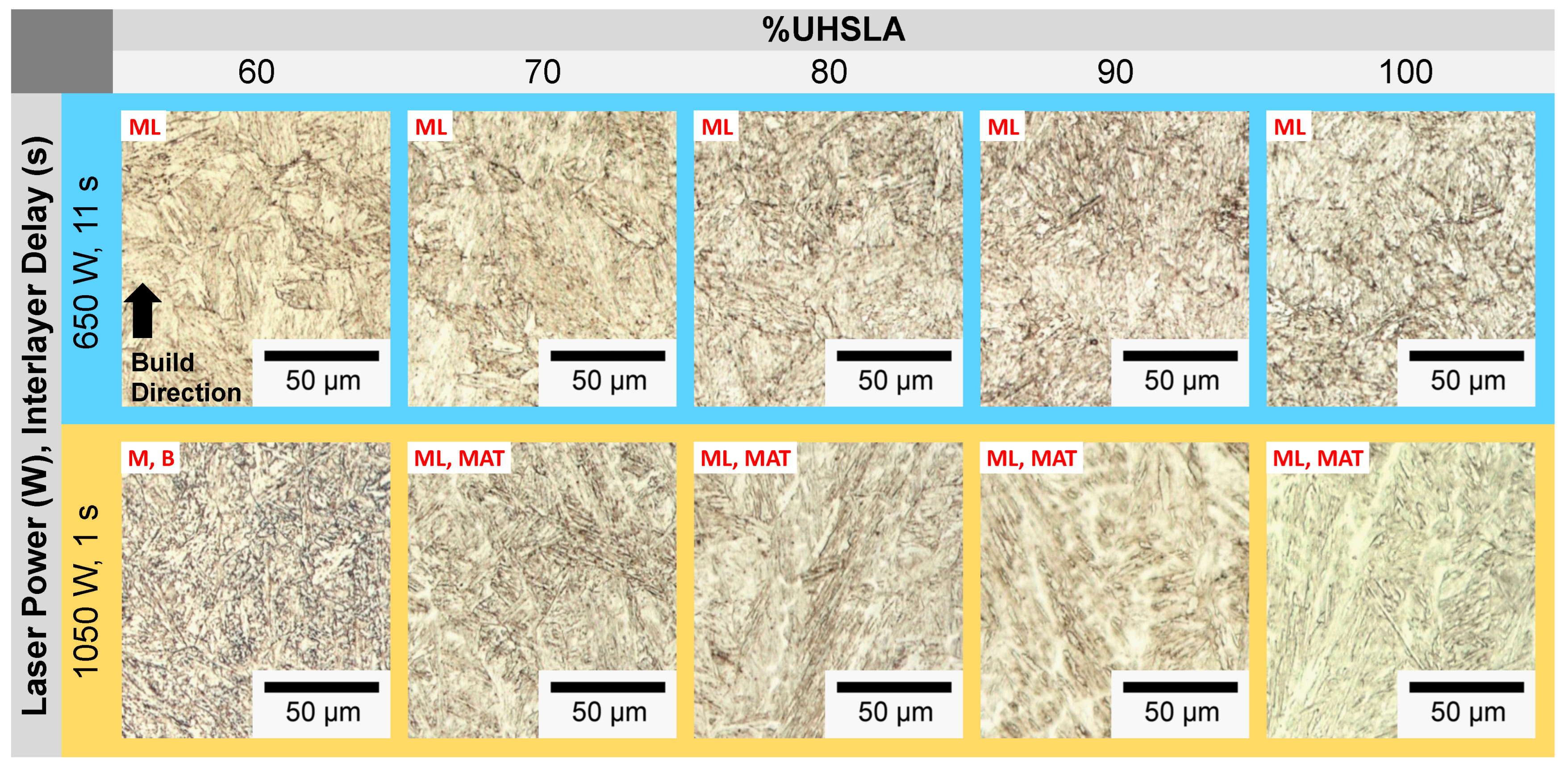
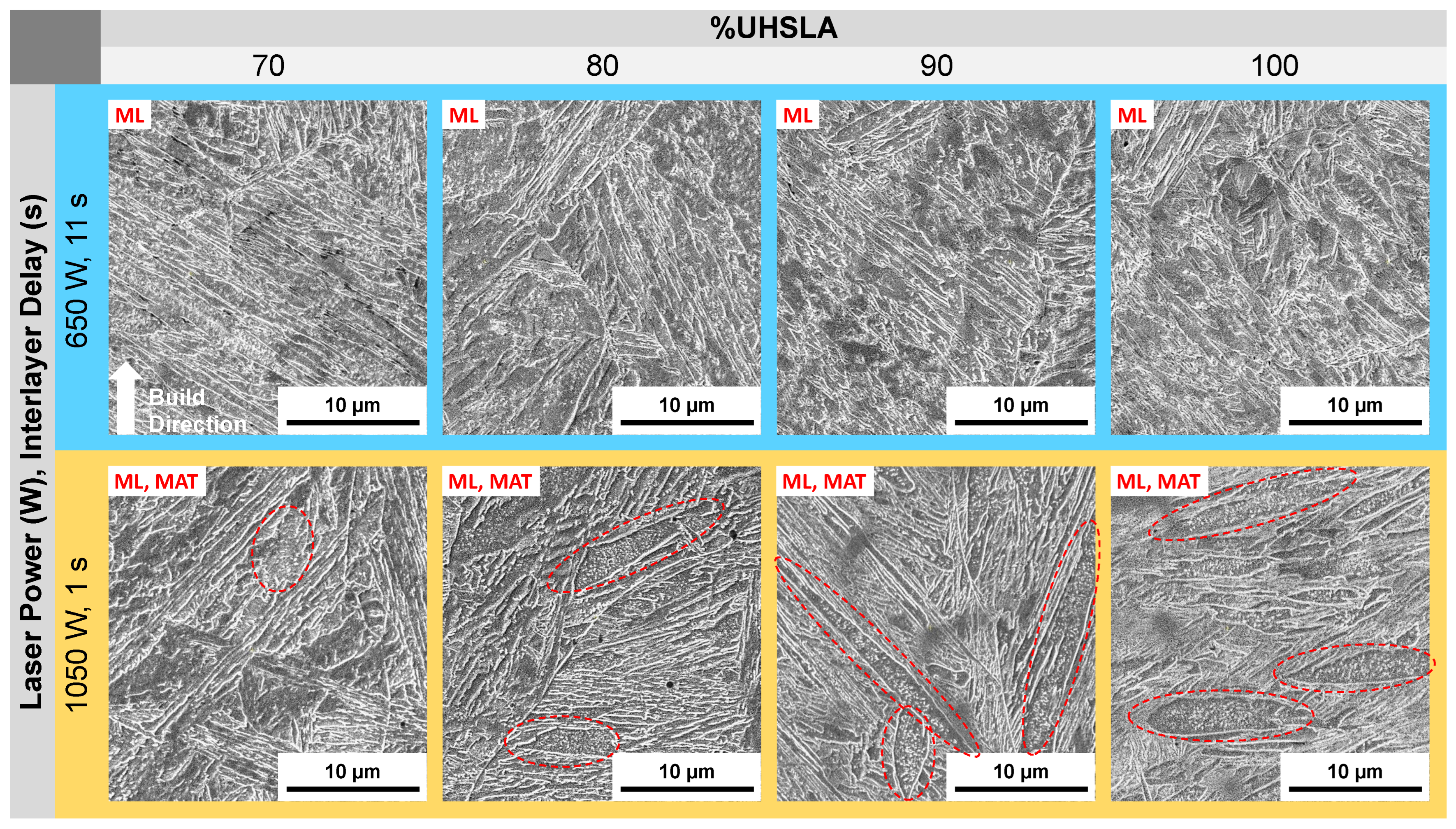
3.7. Microstructure Analysis: Hardness Experiments
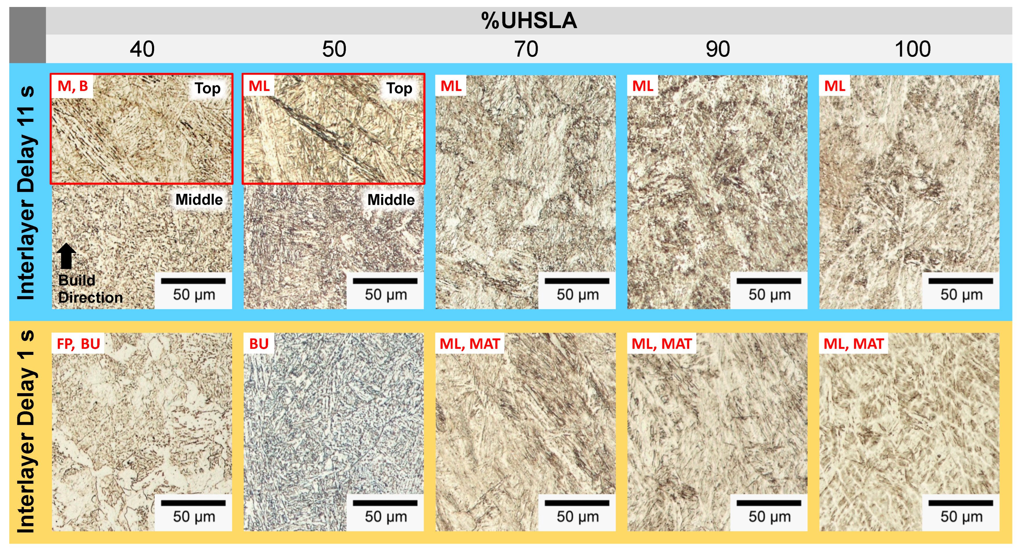
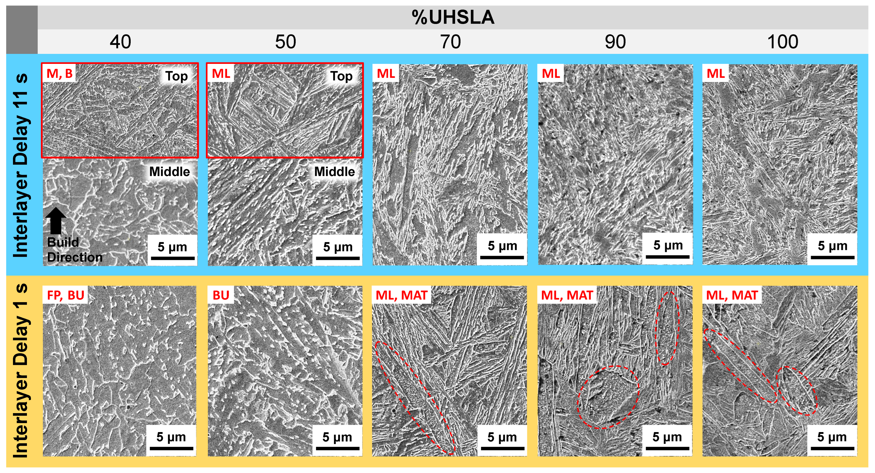
3.8. Microstructure Analysis: Tensile Experiments
3.9. Identifying an Optimal Composition
4. Conclusions
- The hardness, ultimate tensile strength (UTS), and yield strength (YS) of alloys containing 40–50% UHSLA were highly sensitive to process variations, corresponding to cooling rate-driven phase fluctuations between lath martensite and upper bainite.
- Alloys with low UHSLA contents (10–20%) transformed primarily to ferrite; those with high contents (70–100%) transformed to martensite, intermixed with auto-tempered martensite at lower cooling rates. The avoidance of martensite/bainite fluctuations appears to be a key factor leading to improved robustness.
- At 70% UHSLA, the hardness, UTS, and YS were relatively robust, as the alloy content was just high enough to ensure transformation to martensite or auto-tempered martensite. This alloy maintained a relatively high hardness and strength while exhibiting superior ductility to UHSLA without sacrificing tensile toughness.
- Above 70% UHSLA, the YS sensitivity remained low. In contrast, the UTS sensitivity increased, possibly suggesting a strong response of the work hardening capability to auto-tempering at higher alloy contents.
- While hardness analysis captures certain microstructural sensitivities, it may not reveal other sensitivities relevant to the tensile properties, such as factors influencing the work hardening capability. This is an important consideration when designing experiments to evaluate the robustness of alloys.
Author Contributions
Funding
Data Availability Statement
Conflicts of Interest
References
- Sun, S.; Brandt, M.; Easton, M. Powder bed fusion processes: An overview. In Laser Additive Manufacturing: Materials, Design, Technologies, and Applications; Elsevier Inc.: Amsterdam, The Netherlands, 2017; pp. 55–77. [Google Scholar] [CrossRef]
- Thompson, S.M.; Bian, L.; Shamsaei, N.; Yadollahi, A. An overview of direct laser deposition for additive manufacturing; Part I: Transport phenomena, modeling and diagnostics. Addit. Manuf. 2015, 8, 36–62. [Google Scholar] [CrossRef]
- Gudur, S.; Nagallapati, V.; Pawar, S.; Muvvala, G.; Simhambhatla, S. A study on the effect of substrate heating and cooling on bead geometry in wire arc additive manufacturing and its correlation with cooling rate. Mater. Today Proc. 2021, 41, 431–436. [Google Scholar] [CrossRef]
- Vafadar, A.; Guzzomi, F.; Rassau, A.; Hayward, K. Advances in metal additive manufacturing: A review of common processes, industrial applications, and current challenges. Appl. Sci. 2021, 11, 1213. [Google Scholar] [CrossRef]
- Oliveira, J.P.; Santos, T.G.; Miranda, R.M. Revisiting fundamental welding concepts to improve additive manufacturing: From theory to practice. Prog. Mater. Sci. 2020, 107, 100590. [Google Scholar] [CrossRef]
- Clare, A.T.; Mishra, R.S.; Merklein, M.; Tan, H.; Todd, I.; Chechik, L.; Li, J.; Bambach, M. Alloy design and adaptation for additive manufacture. J. Mater. Process. Technol. 2022, 299, 117358. [Google Scholar] [CrossRef]
- Wei, H.; Mukherjee, T.; Zhang, W.; Zuback, J.; Knapp, G.; De, A.; DebRoy, T. Mechanistic models for additive manufacturing of metallic components. Prog. Mater. Sci. 2021, 116, 100703. [Google Scholar] [CrossRef]
- Shamsaei, N.; Yadollahi, A.; Bian, L.; Thompson, S.M. An overview of direct laser deposition for additive manufacturing; Part II: Mechanical behavior, process parameter optimization and control. Addit. Manuf. 2015, 8, 12–35. [Google Scholar] [CrossRef]
- Zhang, C.; Zhu, J.; Zheng, H.; Li, H.; Liu, S.; Cheng, G.J. A review on microstructures and properties of high entropy alloys manufactured by selective laser melting. Int. J. Extrem. Manuf. 2020, 2, 032003. [Google Scholar] [CrossRef]
- Cooke, S.; Ahmadi, K.; Willerth, S.; Herring, R. Metal additive manufacturing: Technology, metallurgy and modelling. J. Manuf. Process. 2020, 57, 978–1003. [Google Scholar] [CrossRef]
- Mukherjee, T.; Zuback, J.; De, A.; DebRoy, T. Printability of alloys for additive manufacturing. Sci. Rep. 2016, 6, 19717. [Google Scholar] [CrossRef]
- Ackers, M.A.; Messé, O.M.; Hecht, U. Novel approach of alloy design and selection for additive manufacturing towards targeted applications. J. Alloy Compd. 2021, 866, 158965. [Google Scholar] [CrossRef]
- Johnson, L.; Mahmoudi, M.; Zhang, B.; Seede, R.; Huang, X.; Maier, J.T.; Maier, H.J.; Karaman, I.; Elwany, A.; Arróyave, R. Assessing printability maps in additive manufacturing of metal alloys. Acta Mater. 2019, 176, 199–210. [Google Scholar] [CrossRef]
- Harrison, N.J.; Todd, I.; Mumtaz, K. Reduction of micro-cracking in nickel superalloys processed by selective laser melting: A fundamental alloy design approach. Acta Mater. 2015, 94, 59–68. [Google Scholar] [CrossRef]
- Zhang, D.; Prasad, A.; Bermingham, M.J.; Todaro, C.J.; Benoit, M.J.; Patel, M.N.; Qiu, D.; StJohn, D.H.; Qian, M.; Easton, M.A. Grain refinement of alloys in fusion-based additive manufacturing processes. Metall. Mater. Trans. A Phys. Metall. Mater. Sci. 2020, 51, 4341–4359. [Google Scholar] [CrossRef]
- Haines, M.; Plotkowski, A.; Frederick, C.L.; Schwalbach, E.J.; Babu, S.S. A sensitivity analysis of the columnar-to-equiaxed transition for Ni-based superalloys in electron beam additive manufacturing. Comput. Mater. Sci. 2018, 155, 340–349. [Google Scholar] [CrossRef]
- Bandyopadhyay, A.; Traxel, K.D.; Lang, M.; Juhasz, M.; Eliaz, N.; Bose, S. Alloy design via additive manufacturing: Advantages, challenges, applications and perspectives. Mater. Today 2022, 52, 207–224. [Google Scholar] [CrossRef]
- Mosallanejad, M.H.; Niroumand, B.; Aversa, A.; Saboori, A. In-situ alloying in laser-based additive manufacturing processes: A critical review. J. Alloy Compd. 2021, 872, 159567. [Google Scholar] [CrossRef]
- Vecchio, K.S.; Dippo, O.F.; Kaufmann, K.R.; Liu, X. High-throughput rapid experimental alloy development (HT-READ). Acta Mater. 2021, 221, 117352. [Google Scholar] [CrossRef]
- Knoll, H.; Ocylok, S.; Weisheit, A.; Springer, H.; Jägle, E.; Raabe, D. Combinatorial alloy design by laser additive manufacturing. Steel Res. Int. 2017, 88, 1600416. [Google Scholar] [CrossRef]
- Lauhoff, C.; Arold, T.; Bolender, A.; Rackel, M.W.; Pyczak, F.; Weinmann, M.; Xu, W.; Molotnikov, A.; Niendorf, T. Microstructure of an additively manufactured Ti-Ta-Al alloy using novel pre-alloyed powder feedstock material. Addit. Manuf. Lett. 2023, 6, 100144. [Google Scholar] [CrossRef]
- Wang, X.; Xiong, W. Uncertainty quantification and composition optimization for alloy additive manufacturing through a CALPHAD-based ICME framework. NPJ Comput. Mater. 2020, 6, 188. [Google Scholar] [CrossRef]
- Sun, Z.; Ma, Y.; Ponge, D.; Zaefferer, S.; Jägle, E.A.; Gault, B.; Rollett, A.D.; Raabe, D. Thermodynamics-guided alloy and process design for additive manufacturing. Nat. Commun. 2022, 13, 4361. [Google Scholar] [CrossRef] [PubMed]
- Gong, W.; Khoshnevisan, S.; Juang, C.H. Gradient-based design robustness measure for robust geotechnical design. Can. Geotech. J. 2014, 51, 1331–1342. [Google Scholar] [CrossRef]
- Sharma, G.; Allen, J.K.; Mistree, F. Classification and execution of coupled decision problems in engineering design for exploration of robust design solutions. In Proceedings of the International Design Engineering Technical Conferences and Computers and Information in Engineering Conference, Anaheim, CA, USA, 18–21 August 2019; Volume 2A: 45th Design Automation Conference. American Society of Mechanical Engineers: New York, NY, USA, 2019; p. V02AT03A019. [Google Scholar] [CrossRef]
- Sagar, V.R.; Lorin, S.; Warmefjord, K.; Soderberg, R. A robust design perspective on factors influencing geometric quality in metal additive manufacturing. J. Manuf. Sci. Eng. Trans. ASME 2021, 143, 071011. [Google Scholar] [CrossRef]
- Hu, Z.; Mahadevan, S. Uncertainty quantification and management in additive manufacturing: Current status, needs, and opportunities. Int. J. Adv. Manuf. Technol. 2017, 93, 2855–2874. [Google Scholar] [CrossRef]
- Pham, T.; Hoang, T.; Tran, X.; Fetni, S.; Duchêne, L.; Tran, H.S.; Habraken, A. A framework for the robust optimization under uncertainty in additive manufacturing. J. Manuf. Process. 2023, 103, 53–63. [Google Scholar] [CrossRef]
- Wang, Z.; Liu, P.; Xiao, Y.; Cui, X.; Hu, Z.; Chen, L. A data-driven approach for process optimization of metallic additive manufacturing under uncertainty. J. Manuf. Sci. Eng. Trans. ASME 2019, 141, 081004. [Google Scholar] [CrossRef]
- Feenstra, D.R.; Molotnikov, A.; Birbilis, N. Utilisation of artificial neural networks to rationalise processing windows in directed energy deposition applications. Mater. Des. 2021, 198, 109342. [Google Scholar] [CrossRef]
- Jardin, R.T.; Tuninetti, V.; Tchuindjang, J.T.; Hashemi, N.; Carrus, R.; Mertens, A.; Duchêne, L.; Tran, H.S.; Habraken, A.M. Sensitivity analysis in the modeling of a high-speed, steel, thin wall produced by directed energy deposition. Metals 2020, 10, 1554. [Google Scholar] [CrossRef]
- Gheysen, J.; Marteleur, M.; van der Rest, C.; Simar, A. Efficient optimization methodology for laser powder bed fusion parameters to manufacture dense and mechanically sound parts validated on AlSi12 alloy. Mater. Des. 2021, 199, 109433. [Google Scholar] [CrossRef]
- Stavropoulos, P.; Papacharalampopoulos, A.; Michail, C.K.; Chryssolouris, G. Robust additive manufacturing performance through a control oriented digital twin. Metals 2021, 11, 708. [Google Scholar] [CrossRef]
- Cheng, H.; Luo, X.; Wu, X. Recent research progress on additive manufacturing of high-strength low-alloy steels: Focusing on the processing parameters, microstructures and properties. Mater. Today Commun. 2023, 36, 106616. [Google Scholar] [CrossRef]
- Wang, Z.; Sun, G.; Chen, M.; Lu, Y.; Zhang, S.; Lan, H.; Bi, K.; Ni, Z. Investigation of the underwater laser directed energy deposition technique for the on-site repair of HSLA-100 steel with excellent performance. Addit. Manuf. 2021, 39, 101884. [Google Scholar] [CrossRef]
- Wang, Z.; Yang, K.; Chen, M.; Lu, Y.; Wang, S.; Wu, E.; Bi, K.; Ni, Z.; Sun, G. High-quality remanufacturing of HSLA-100 steel through the underwater laser directed energy deposition in an underwater hyperbaric environment. Surf. Coatings Technol. 2022, 437, 128370. [Google Scholar] [CrossRef]
- Bhadeshia, H.; Honeycombe, R. Steels: Microstructure and Properties, 4th ed.; Elsevier: Oxford, UK, 2017. [Google Scholar]
- Shao, Y.; Liu, C.; Yan, Z.; Li, H.; Liu, Y. Formation mechanism and control methods of acicular ferrite in HSLA steels: A review. J. Mater. Sci. Technol. 2018, 34, 737–744. [Google Scholar] [CrossRef]
- Kim, N.J. The physical metallurgy of HSLA linepipe steels—A review. JOM 1983, 35, 21–27. [Google Scholar] [CrossRef]
- Jun, H.; Kang, J.; Seo, D.; Kang, K.; Park, C. Effects of deformation and boron on microstructure and continuous cooling transformation in low carbon HSLA steels. Mater. Sci. Eng. A 2006, 422, 157–162. [Google Scholar] [CrossRef]
- Talaş, Ş. The assessment of carbon equivalent formulas in predicting the properties of steel weld metals. Mater. Des. (1980–2015) 2010, 31, 2649–2653. [Google Scholar] [CrossRef]
- Kasuya, T.; Yurioka, N. Carbon equivalent and multiplying factor for hardenability of steel. Weld. J. 1993, 72, 263–268. [Google Scholar]
- Barr, C.; Rahman Rashid, R.A.; Palanisamy, S.; Watts, J.; Brandt, M. Examination of steel compatibility with additive manufacturing and repair via laser directed energy deposition. J. Laser Appl. 2023, 35, 022015. [Google Scholar] [CrossRef]
- Wang, Z.; Chen, M.; Zhao, K.; Li, R.; Zong, L.; Zhang, S.; Sun, G. Effect of different feedstocks on the microstructure and mechanical properties of HSLA steel repaired by underwater laser direct metal deposition. Mater. Chem. Phys. 2024, 314, 128935. [Google Scholar] [CrossRef]
- Kelley, J.P.; Newkirk, J.W.; Bartlett, L.N.; Sparks, T.; Isanaka, S.P.; Alipour, S.; Liou, F. Influence of steel alloy composition on the process robustness of as-built hardness in laser-directed energy deposition. In Proceedings of the 34th Annual International Solid Freeform Fabrication Symposium, Austin, TX, USA, 14–16 August 2023; pp. 494–513. [Google Scholar] [CrossRef]
- Alexopoulos, E.C. Introduction to multivariate regression analysis. Hippokratia 2010, 14 (Suppl. 1), 23–28. [Google Scholar]
- Bowerman, B.L.; O’Connell, R.T.; Murphree, E.S. Regression Analysis: Unified Concepts, Practical Applications, and Computer Implementation, 1st ed.; Business Expert Press: New York, NY, USA, 2015. [Google Scholar]
- JMP Statistical Discovery. Scaled Estimates and the Coding of Continuous Terms. 2018. Available online: https://www.jmp.com/support/help/14/scaled-estimates-and-the-coding-of-continuous-te.shtml (accessed on 15 September 2024).
- Liu, S.; Zhang, Y.; Kovacevic, R. Numerical simulation and experimental study of powder flow distribution in high power direct diode laser cladding process. Lasers Manuf. Mater. Process. 2015, 2, 199–218. [Google Scholar] [CrossRef]
- Takeuchi, A.; Inoue, A. Classification of bulk metallic glasses by atomic size difference, heat of mixing and period of constituent elements and its application to characterization of the main alloying element. Mater. Trans. 2005, 46, 2817–2829. [Google Scholar] [CrossRef]
- Li, W.; Chen, X.; Yan, L.; Zhang, J.; Zhang, X.; Liou, F. Additive manufacturing of a new Fe-Cr-Ni alloy with gradually changing compositions with elemental powder mixes and thermodynamic calculation. Int. J. Adv. Manuf. Technol. 2018, 95, 1013–1023. [Google Scholar] [CrossRef]
- ASTM E92-17; Standard Test Methods for Vickers Hardness and Knoop Hardness of Metallic Materials. ASTM International: West Conshohocken, PA, USA, 2017. [CrossRef]
- Newbury, D.E.; Ritchie, N.W. Is scanning electron microscopy/energy dispersive X-ray spectrometry (SEM/EDS) quantitative? Scanning 2013, 35, 141–168. [Google Scholar] [CrossRef]
- Karnati, S.; Axelsen, I.; Liou, F.W.; Newkirk, J.W. Investigation of tensile properties of bulk and SLM fabricated 304L stainless steel using various gage length specimens. In Proceedings of the 27th Annual International Solid Freeform Fabrication Symposium, Austin, TX, USA, 8–10 August 2016; University of Texas at Austin: Austin, TX, USA, 2016; pp. 592–604. [Google Scholar]
- Chen, Z.; Gandhi, U.; Lee, J.; Wagoner, R. Variation and consistency of Young’s modulus in steel. J. Mater. Process. Technol. 2016, 227, 227–243. [Google Scholar] [CrossRef]
- Kiran, A.; Koukolíková, M.; Vavřík, J.; Urbánek, M.; Džugan, J. Base plate preheating effect on microstructure of 316L stainless steel single track deposition by directed energy deposition. Materials 2021, 14, 5129. [Google Scholar] [CrossRef]
- Xia, Z.; Xu, J.; Shi, J.; Shi, T.; Sun, C.; Qiu, D. Microstructure evolution and mechanical properties of reduced activation steel manufactured through laser directed energy deposition. Addit. Manuf. 2020, 33, 101114. [Google Scholar] [CrossRef]
- Crespo, A.; Vilar, R. Finite element analysis of the rapid manufacturing of Ti–6Al–4V parts by laser powder deposition. Scr. Mater. 2010, 63, 140–143. [Google Scholar] [CrossRef]
- ASTM E140-12b; Standard Hardness Conversion Tables for Metals Relationship among Brinell Hardness, Vickers Hardness, Rockwell Hardness, Superficial Hardness, Knoop Hardness, Scleroscope Hardness, and Leeb Hardness. ASTM International: West Conshohocken, PA, USA, 2019. [CrossRef]
- Kou, S. Welding Metallurgy, 2nd ed.; John Wiley & Sons, Inc.: Hoboken, NJ, USA, 2003. [Google Scholar]
- Mendagaliev, R.; Ivanov, S.; Babkin, K.; Lebedeva, N.; Klimova-Korsmik, O.; Turichin, G. Influence of the thermal cycle on microstructure formation during direct laser deposition of bainite-martensitic steel. Mater. Chem. Phys. 2023, 300, 127523. [Google Scholar] [CrossRef]
- Yang, Z.G.; Fang, H.S. An overview on bainite formation in steels. Curr. Opin. Solid State Mater. Sci. 2005, 9, 277–286. [Google Scholar] [CrossRef]
- Macchi, J.; Geandier, G.; Teixeira, J.; Denis, S.; Bonnet, F.; Allain, S.Y. Time-resolved in-situ dislocation density evolution during martensitic transformation by high-energy-XRD experiments: A study of C content and cooling rate effects. Materialia 2022, 26, 101577. [Google Scholar] [CrossRef]
- Sohrabi, M.; Mirzadeh, H.; Mehranpour, M.; Heydarinia, A.; Razi, R. Aging kinetics and mechanical properties of copper-bearing low-carbon HSLA-100 microalloyed steel. Arch. Civ. Mech. Eng. 2019, 19, 1409–1418. [Google Scholar] [CrossRef]
- Salemi, A.; Abdollah-zadeh, A. The effect of tempering temperature on the mechanical properties and fracture morphology of a NiCrMoV steel. Mater. Charact. 2008, 59, 484–487. [Google Scholar] [CrossRef]
- Kang, J.; Wang, Y.; Chen, X.; Zhang, C.; Peng, Y.; Wang, T. Grain refinement and mechanical properties of Fe-30Mn-0.11C steel. Results Phys. 2019, 13, 102247. [Google Scholar] [CrossRef]
- Su, Y.; Song, R.; Wang, T.; Cai, H.; Wen, J.; Guo, K. Grain size refinement and effect on the tensile properties of a novel low-cost stainless steel. Mater. Lett. 2020, 260, 126919. [Google Scholar] [CrossRef]
- Qiao, G.y.; Han, X.l.; Chen, X.w.; Wang, X.; Liao, B.; Xiao, F.r. Transformation of M/A constituents during tempering and its effects on impact toughness of weld metals for X80 hot bends. Adv. Mater. Sci. Eng. 2019, 2019, 6429045. [Google Scholar] [CrossRef]
- Peng, J.; Huang, C.; Liu, F.; Zhang, B.; Liu, F. Effect of Deposition Thickness on the Microstructure of Laser Solid Forming 34CrNiMo6 Steel. J. Mater. Eng. Perform. 2024, 33, 1693–1703. [Google Scholar] [CrossRef]
- Liu, F.; Lin, X.; Shi, J.; Zhang, Y.; Bian, P.; Li, X.; Hu, Y. Effect of microstructure on the Charpy impact properties of directed energy deposition 300M steel. Addit. Manuf. 2019, 29, 100795. [Google Scholar] [CrossRef]
- Kang, X.; Dong, S.; Men, P.; Liu, X.; Yan, S.; Wang, H.; Xu, B. Microstructure evolution and gradient performance of 24CrNiMo steel prepared via laser melting deposition. Mater. Sci. Eng. A 2020, 777, 139004. [Google Scholar] [CrossRef]
- Babu, S.R.; Nyyssönen, T.; Jaskari, M.; Järvenpää, A.; Davis, T.P.; Pallaspuro, S.; Kömi, J.; Porter, D. Observations on the relationship between crystal orientation and the level of auto-tempering in an as-quenched martensitic steel. Metals 2019, 9, 1255. [Google Scholar] [CrossRef]
- Panchenko, O.; Kladov, I.; Kurushkin, D.; Zhabrev, L.; Ryl’kov, E.; Zamozdra, M. Effect of thermal history on microstructure evolution and mechanical properties in wire arc additive manufacturing of HSLA steel functionally graded components. Mater. Sci. Eng. A 2022, 851, 143569. [Google Scholar] [CrossRef]
- Wang, J.; Diao, C.; Taylor, M.; Wang, C.; Pickering, E.; Ding, J.; Pimentel, M.; Williams, S. Investigation of 300M ultra-high-strength steel deposited by wire-based gas metal arc additive manufacturing. Int. J. Adv. Manuf. Technol. 2023, 129, 3751–3767. [Google Scholar] [CrossRef]
- Zou, X.; Yan, Z.; Zou, K.; Liu, W.; Song, L.; Li, S.; Cha, L. Grain refinement by dynamic recrystallization during laser direct energy deposition of 316L stainless steel under thermal cycles. J. Manuf. Process. 2022, 76, 646–655. [Google Scholar] [CrossRef]
- Hu, Y.; Lin, X.; Li, Y.; Zhang, S.; Gao, X.; Liu, F.; Li, X.; Huang, W. Plastic deformation behavior and dynamic recrystallization of Inconel 625 superalloy fabricated by directed energy deposition. Mater. Des. 2020, 186, 108359. [Google Scholar] [CrossRef]
- Tkachev, E.; Borisov, S.; Belyakov, A.; Kniaziuk, T.; Vagina, O.; Gaidar, S.; Kaibyshev, R. Effect of quenching and tempering on structure and mechanical properties of a low-alloy 0.25 C steel. Mater. Sci. Eng. A 2023, 868, 144757. [Google Scholar] [CrossRef]
- Mathevon, A.; Fabrègue, D.; Massardier, V.; Cazottes, S.; Rocabois, P.; Perez, M. Investigation and mean-field modelling of microstructural mechanisms driving the tensile properties of dual-phase steels. Mater. Sci. Eng. A 2021, 822, 141532. [Google Scholar] [CrossRef]
- Malheiros, L.C.; Rodriguez, E.P.; Arlazarov, A. Mechanical behavior of tempered martensite: Characterization and modeling. Mater. Sci. Eng. A 2017, 706, 38–47. [Google Scholar] [CrossRef]
Disclaimer/Publisher’s Note: The statements, opinions and data contained in all publications are solely those of the individual author(s) and contributor(s) and not of MDPI and/or the editor(s). MDPI and/or the editor(s) disclaim responsibility for any injury to people or property resulting from any ideas, methods, instructions or products referred to in the content. |
© 2024 by the authors. Licensee MDPI, Basel, Switzerland. This article is an open access article distributed under the terms and conditions of the Creative Commons Attribution (CC BY) license (https://creativecommons.org/licenses/by/4.0/).
Share and Cite
Kelley, J.; Newkirk, J.W.; Bartlett, L.N.; Isanaka, S.P.; Sparks, T.; Alipour, S.; Liou, F. Development of Robust Steel Alloys for Laser-Directed Energy Deposition via Analysis of Mechanical Property Sensitivities. Micromachines 2024, 15, 1180. https://doi.org/10.3390/mi15101180
Kelley J, Newkirk JW, Bartlett LN, Isanaka SP, Sparks T, Alipour S, Liou F. Development of Robust Steel Alloys for Laser-Directed Energy Deposition via Analysis of Mechanical Property Sensitivities. Micromachines. 2024; 15(10):1180. https://doi.org/10.3390/mi15101180
Chicago/Turabian StyleKelley, Jonathan, Joseph W. Newkirk, Laura N. Bartlett, Sriram Praneeth Isanaka, Todd Sparks, Saeid Alipour, and Frank Liou. 2024. "Development of Robust Steel Alloys for Laser-Directed Energy Deposition via Analysis of Mechanical Property Sensitivities" Micromachines 15, no. 10: 1180. https://doi.org/10.3390/mi15101180