
Enhanced DMA Test Procedure to Measure Viscoelastic Properties of Epoxy-Based Molding Compound: Multiple Oscillatory Strain Amplitudes and Monotonic Loading

Abstract
1. Introduction
2. Relationship Between Time Domain Analysis and Frequency Domain Analysis
2.1. Time Domain Analysis for Thermorheologically Simple (TRS) Materials
2.2. Frequency DomainAnalysis for TRS Materials
2.2.1. Relationship Between Relaxation Modulus and Complex Modulus
2.2.2. Experimental Practice of TRS in the Frequency Domain
3. Challenges Associated with Materials with Extreme Temperature Dependency
Extreme Change in Moduli over Testing Temperature
4. Enhanced Procedure with Multiple Oscillatory Amplitudes and Monotonic Loading
4.1. Proposed Procedure
4.2. Implementation
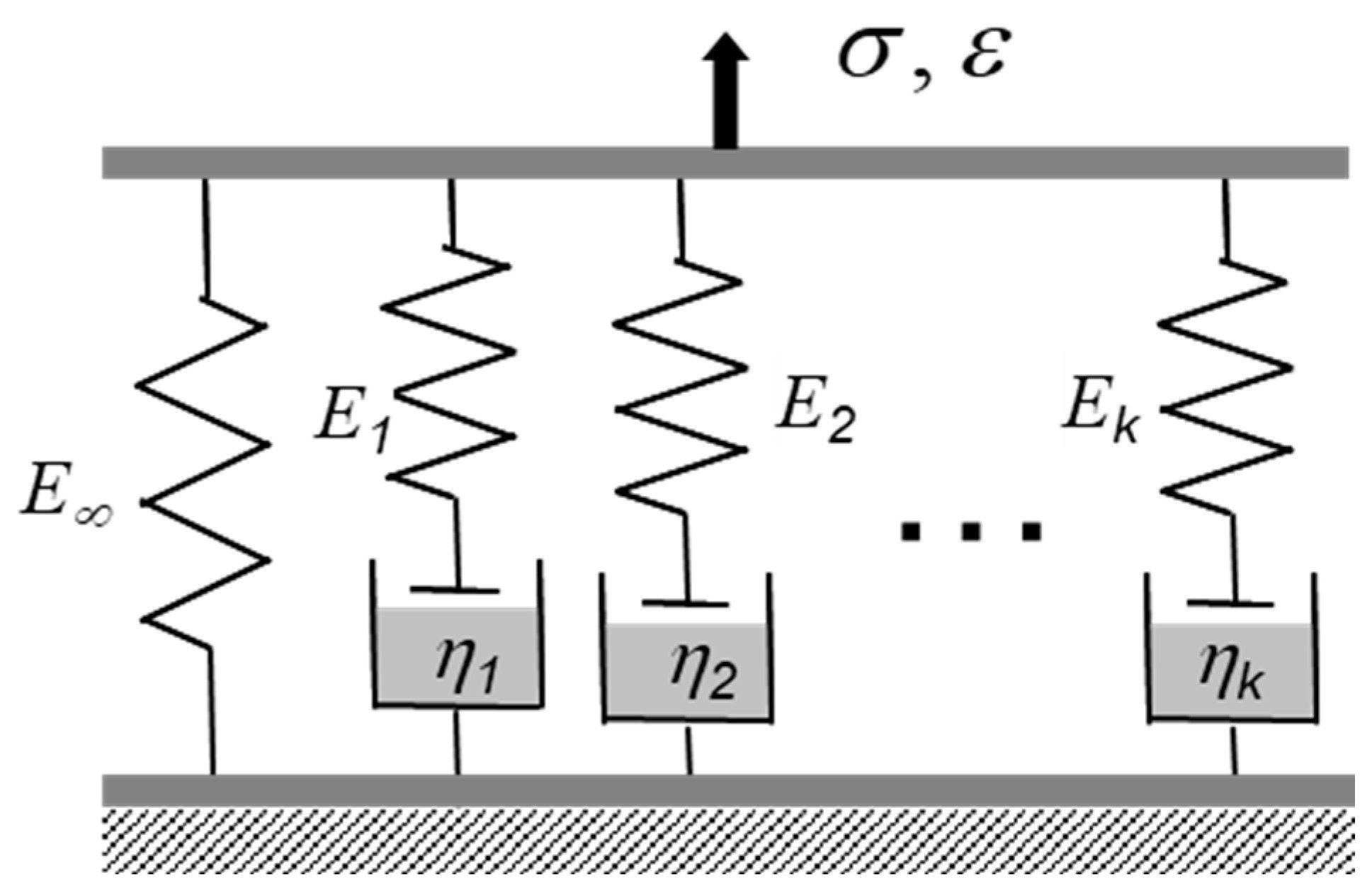
4.3. Determination of Generalized Maxwell Model Constants
5. Discussions
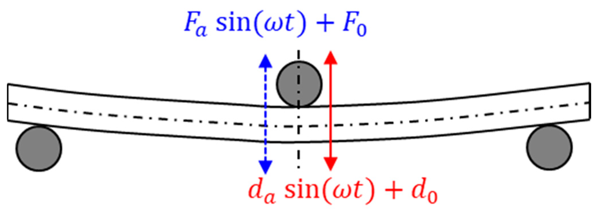
5.1. Virtual Testing Using the Relaxation Modulus
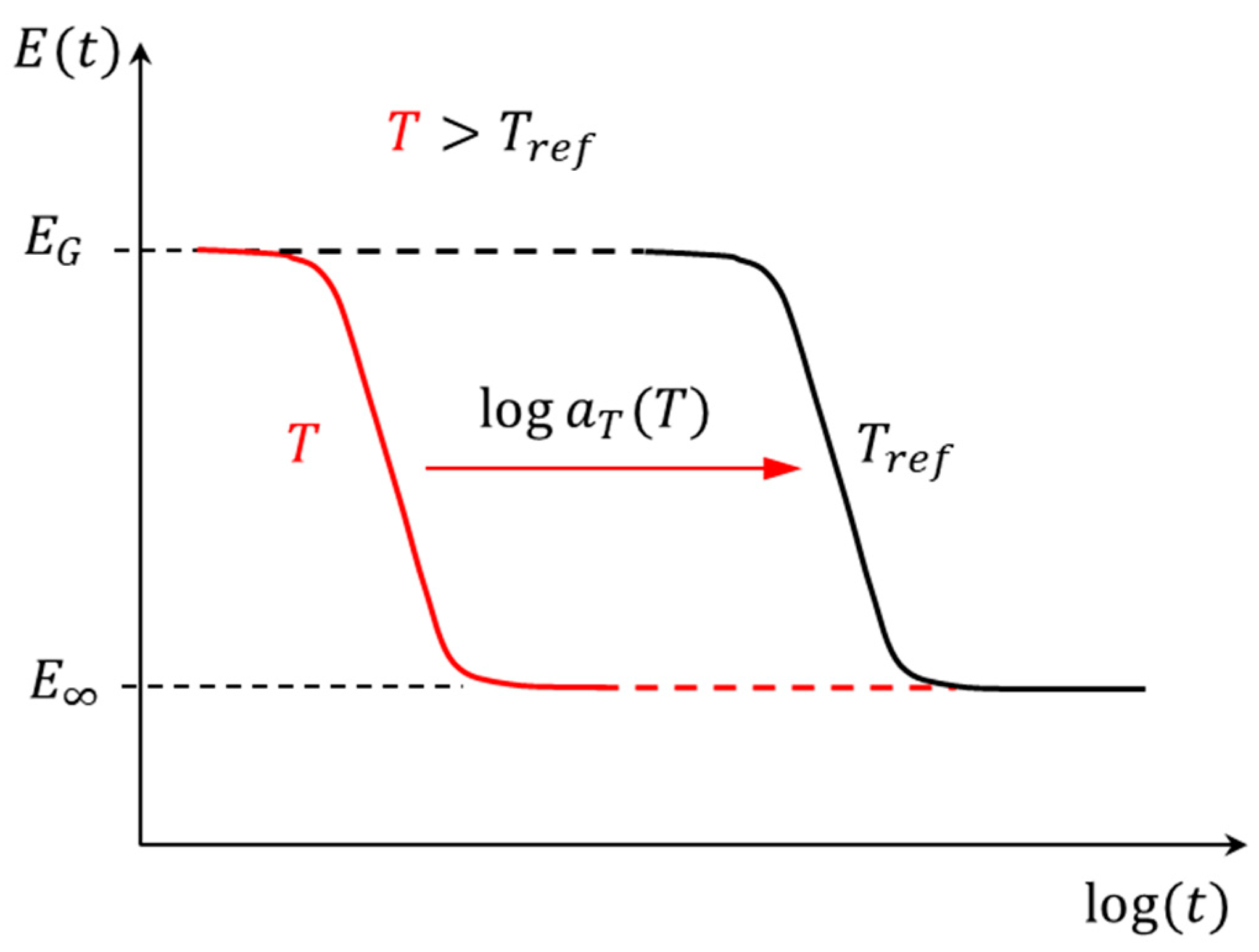
5.2. Master Curve Calculation with Horizontal and Vertical Shifting
6. Conclusions
Author Contributions
Funding
Data Availability Statement
Acknowledgments
Conflicts of Interest
List of Abbreviations
| DMA | dynamic mechanical analysis |
| EMC | epoxy-based molding compound |
| TTS | time–temperature superposition |
| FO-WLP | fan-out wafer-level packaging |
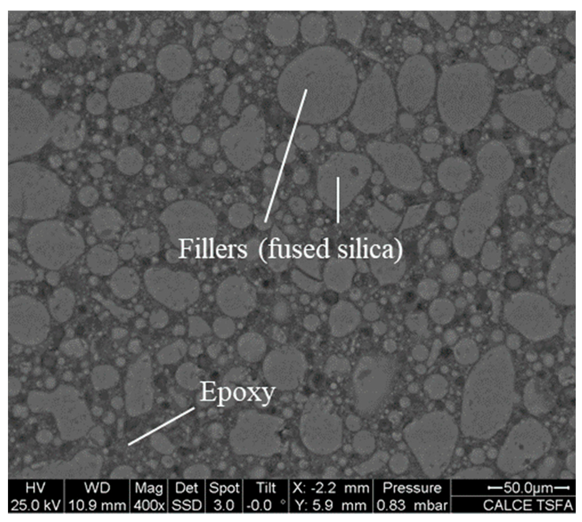
| SEM | scanning electron microscope |
| LVE | linear viscoelasticity |
| TRS | thermorheological simplicity |
| MFT | multi-frequency temperature |
Appendix A. MATLAB Codes
- I.
- The MATLAB code used for fitting the master curve
- II.
- The MATLAB code used to plot the master curve in the time domain
References
- Phansalkar, S.P.; Han, B.; Akbari, E.; Vaitiekunas, P. On the Viscoelastic Property Measurement of Filled Polymers by Dynamic Mechanical Analyzer (DMA). In International Electronic Packaging Technical Conference and Exhibition; American Society of Mechanical Engineers: New York, NY, USA, 2022; Volume 86577, p. V001T005A004. [Google Scholar]
- Yadav, S. Analysis of Glass Transition Temperature of PCB & Substrate Using Dynamic Mechanical Analysis & Thermomechanical Analysis; University of Texas: Arlington, TX, USA, 2020. [Google Scholar]
- Phansalkar, S.; Kim, C.; Han, B. Mechanical Characterization of Dual Curable Adhesives. In Proceedings of the 2020 IEEE 70th Electronic Components and Technology Conference (ECTC), Orlando, FL, USA, 3–30 June 2020; pp. 1094–1099. [Google Scholar]
- Li, D.D.; Li, S.; Zhang, S.; Liu, X.W.; Wong, C.P. Thermo and dynamic mechanical properties of the high refractive index silicone resin for light emitting diode packaging. IEEE Trans. Compon. Packag. Manuf. Technol. 2013, 4, 190–197. [Google Scholar]
- Niu, L.; Yang, D.; Zhang, G. Characterization, modelling, and parameter sensitivity study on electronic packaging polymers. In Proceedings of the 2009 International Conference on Electronic Packaging Technology & High Density Packaging, Beijing, China, 10–13 August 2009; pp. 763–767. [Google Scholar]
- Menard, K.P.; Menard, N. Dynamic Mechanical Analysis; CRC Press: Boca Raton, FL, USA, 2020. [Google Scholar]
- Brinson, H.F.; Brinson, L.C. Polymer Engineering Science and Viscoelasticity; Springer: Berlin/Heidelberg, Germany, 2015. [Google Scholar]
- Chartoff, R.P.; Menczel, J.D.; Dillman, S.H. Dynamic mechanical analysis (DMA). In Thermal Analysis of Polymers: Fundamentals and Applications; John Wiley & Sons, Inc.: Hoboken, NJ, USA, 2009; pp. 387–495. [Google Scholar]
- Phansalkar, S.P.; Kim, C.; Han, B. Effect of critical properties of epoxy molding compound on warpage prediction: A critical review. Microelectron. Reliab. 2022, 130, 114480. [Google Scholar] [CrossRef]
- Kamath, V.; Mackley, M. The determination of polymer relaxation moduli and memory functions using integral transforms. J. Non-Newton. Fluid Mech. 1989, 32, 119–144. [Google Scholar]
- Tschoegl, N.W.; Knauss, W.G.; Emri, I. Poisson’s ratio in linear viscoelasticity–a critical review. Mech. Time-Depend. Mater. 2002, 6, 3–51. [Google Scholar]
- ASTM D790; Standard Test Methods for Flexural Properties of Unreinforced and Reinforced Plastics and Electrical Insulating Materials. ASTM Standards: West Conshohocken, PA, USA, 1997.
- Chowdhury, P.R.; Suhling, J.C.; Lall, P. Characterization of viscoelastic response of underfill materials. In Proceedings of the 2019 18th IEEE Intersociety Conference on Thermal and Thermomechanical Phenomena in Electronic Systems (ITherm), Las Vegas, NV, USA, 28–31 May 2019; pp. 1321–1331. [Google Scholar]
- Gromala, P. (Mobility Electronics, Engineering Power Electronics (ME-PE/ENG) Division, Robert Bosch GmbH, Reutlingen, Germany). Personal communication, 2021. [Google Scholar]


Disclaimer/Publisher’s Note: The statements, opinions and data contained in all publications are solely those of the individual author(s) and contributor(s) and not of MDPI and/or the editor(s). MDPI and/or the editor(s) disclaim responsibility for any injury to people or property resulting from any ideas, methods, instructions or products referred to in the content. |
© 2025 by the authors. Licensee MDPI, Basel, Switzerland. This article is an open access article distributed under the terms and conditions of the Creative Commons Attribution (CC BY) license (https://creativecommons.org/licenses/by/4.0/).
Share and Cite
Phansalkar, S.P.; Mittakolu, R.; Han, B.; Kim, T. Enhanced DMA Test Procedure to Measure Viscoelastic Properties of Epoxy-Based Molding Compound: Multiple Oscillatory Strain Amplitudes and Monotonic Loading. Micromachines 2025, 16, 384. https://doi.org/10.3390/mi16040384
Phansalkar SP, Mittakolu R, Han B, Kim T. Enhanced DMA Test Procedure to Measure Viscoelastic Properties of Epoxy-Based Molding Compound: Multiple Oscillatory Strain Amplitudes and Monotonic Loading. Micromachines. 2025; 16(4):384. https://doi.org/10.3390/mi16040384
Chicago/Turabian StylePhansalkar, Sukrut Prashant, Roshith Mittakolu, Bongtae Han, and Taehwa Kim. 2025. "Enhanced DMA Test Procedure to Measure Viscoelastic Properties of Epoxy-Based Molding Compound: Multiple Oscillatory Strain Amplitudes and Monotonic Loading" Micromachines 16, no. 4: 384. https://doi.org/10.3390/mi16040384
APA StylePhansalkar, S. P., Mittakolu, R., Han, B., & Kim, T. (2025). Enhanced DMA Test Procedure to Measure Viscoelastic Properties of Epoxy-Based Molding Compound: Multiple Oscillatory Strain Amplitudes and Monotonic Loading. Micromachines, 16(4), 384. https://doi.org/10.3390/mi16040384