
Research on Machining Parameter Optimization and an Electrode Wear Compensation Method of Microgroove Micro-EDM


Abstract
:1. Introduction
2. Experiment Platform and Method
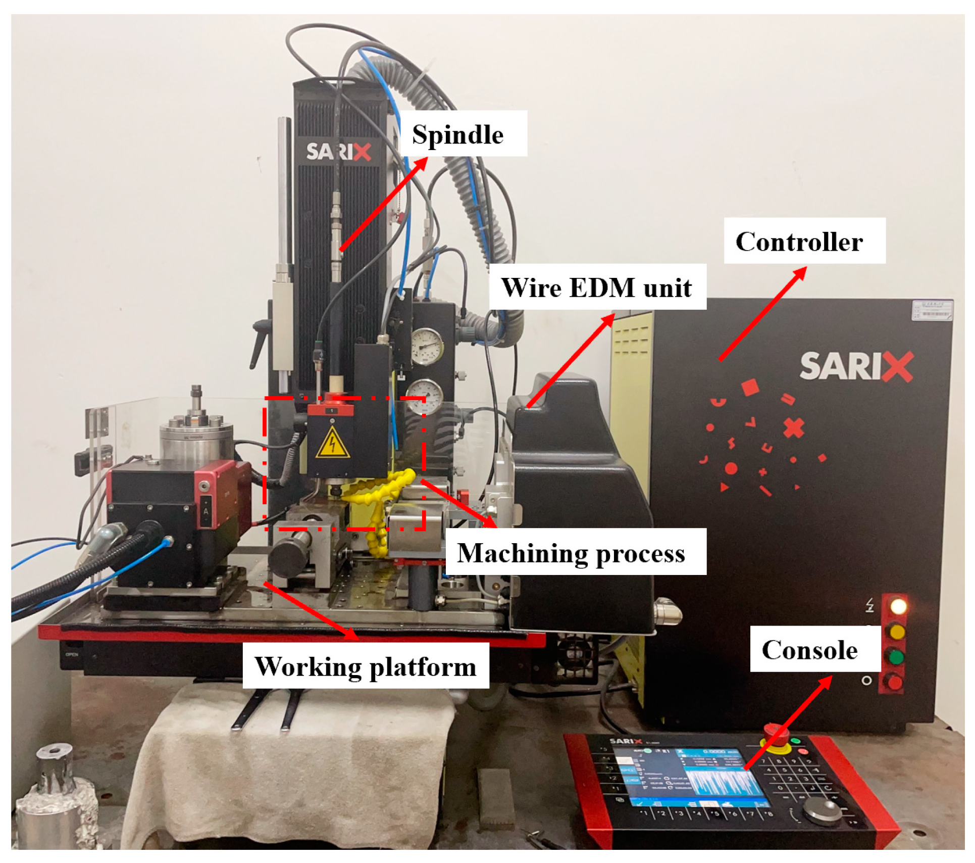
2.1. Experiment Platform
2.2. Grey Relational Analysis
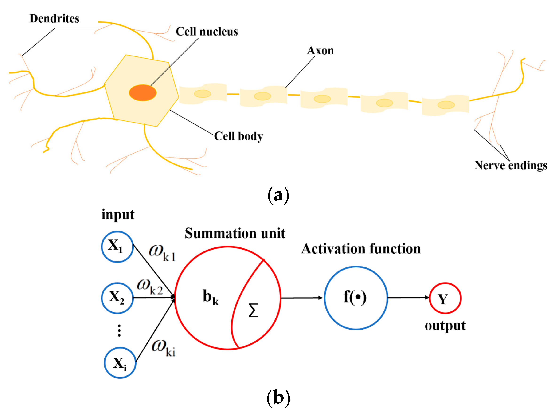
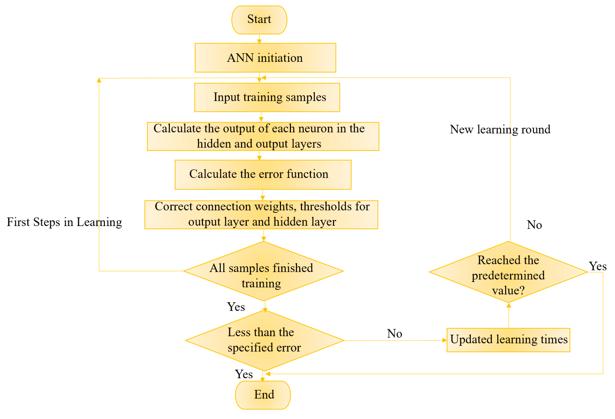
2.3. Artificial Neural Network
2.4. Image Processing Technology
3. Orthogonal Experiment and GRA Multi-Objective Optimization
3.1. Orthogonal Experiment Design and Result Analysis
3.2. GRA Multi-Objective Optimization
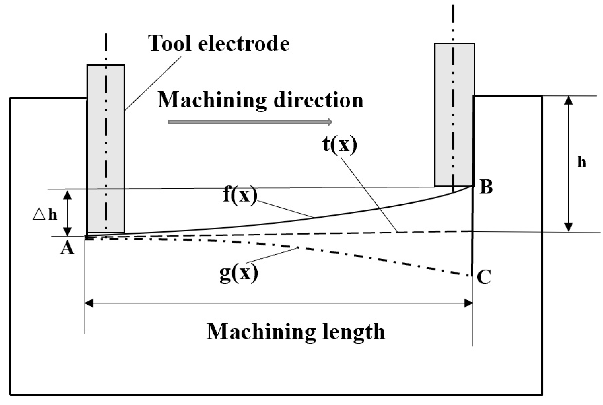
4. Electrode Axial Wear Compensation Experiment
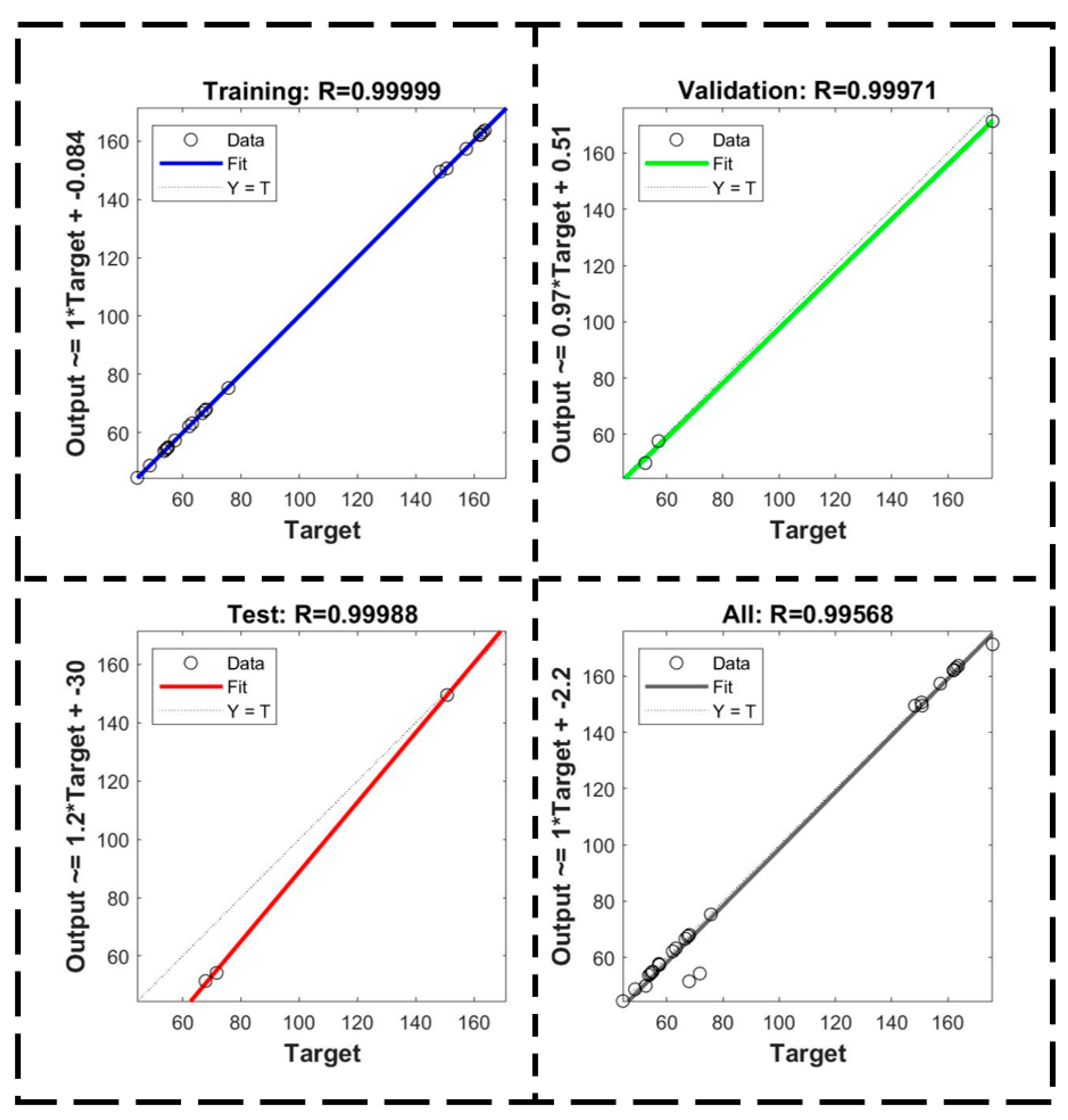
4.1. ANN Prediction Model Establishment
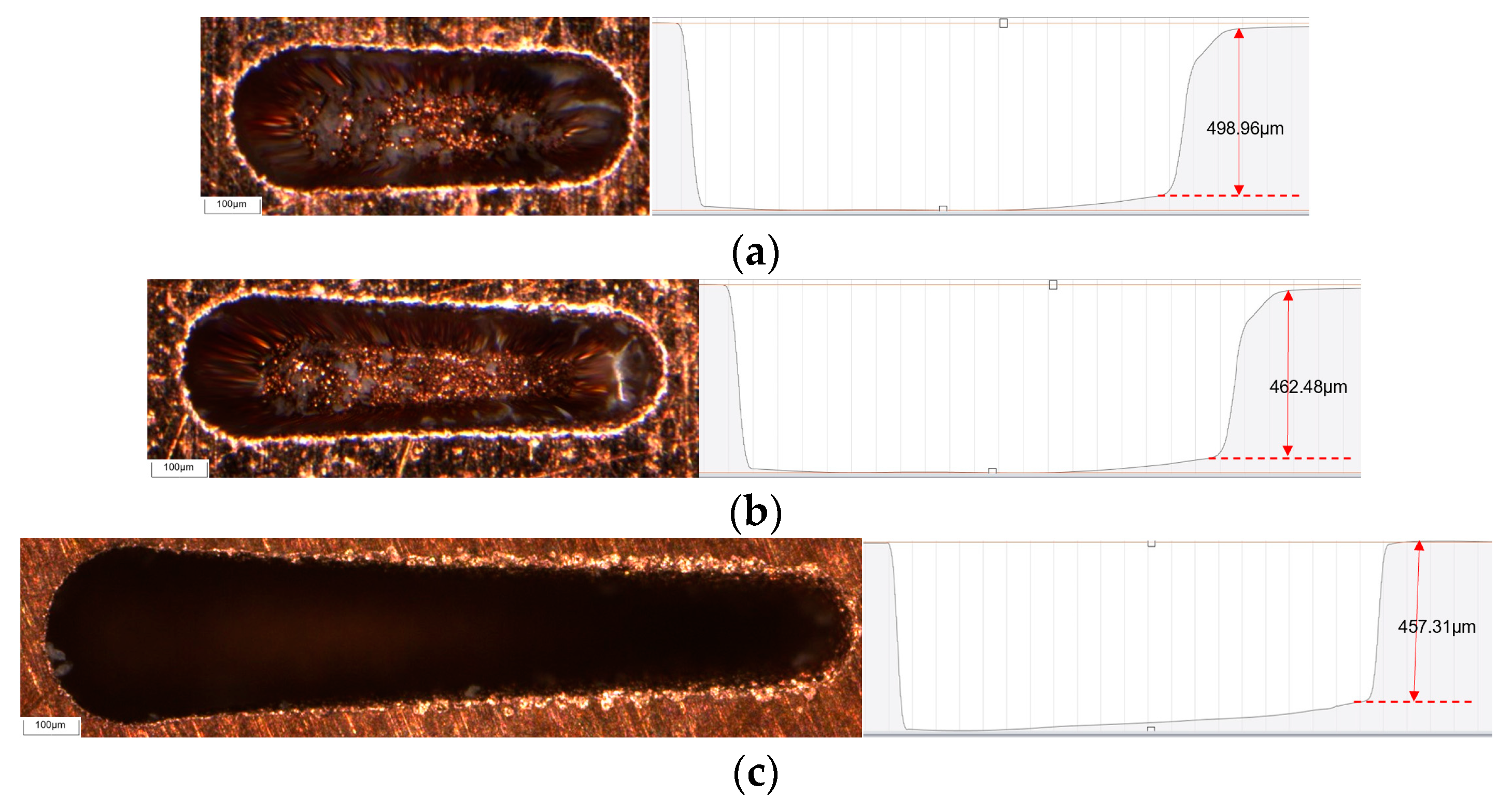
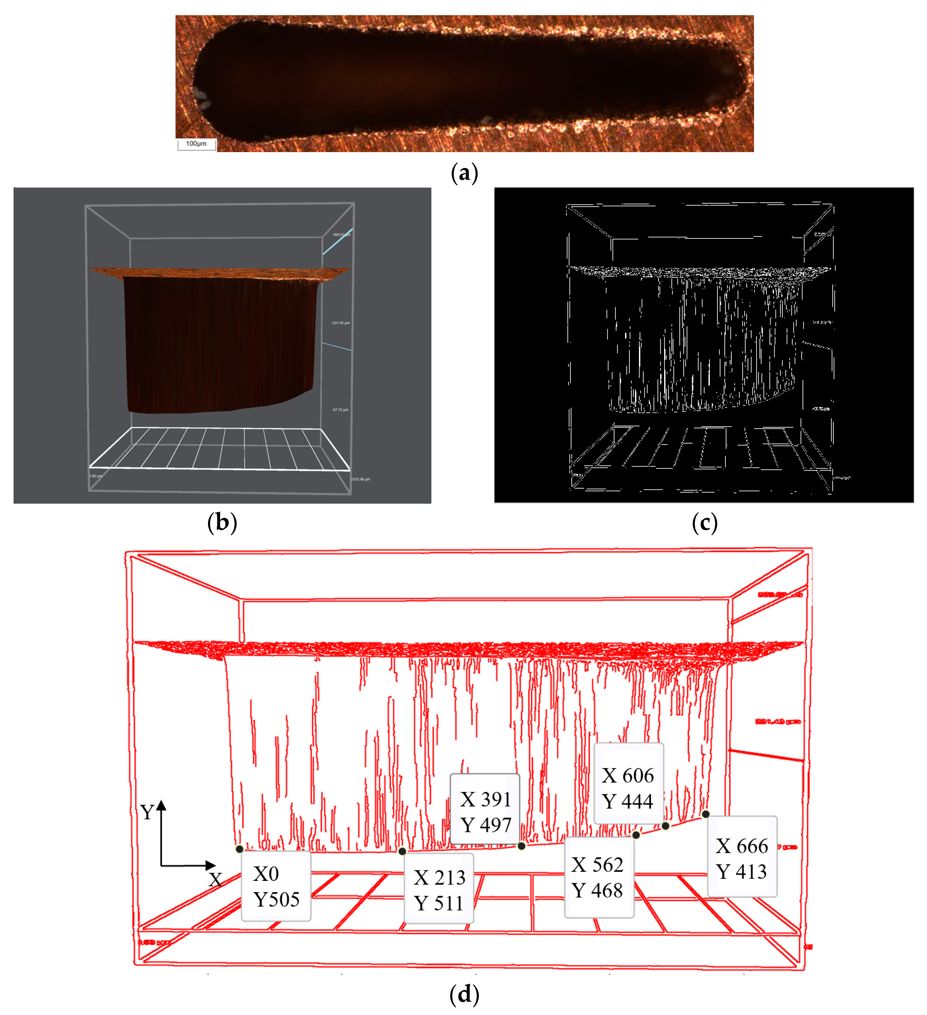
4.2. Image Processing Technology Analysis
- Exponential function
- 2.
- Power function
- 3.
- Polynomial function
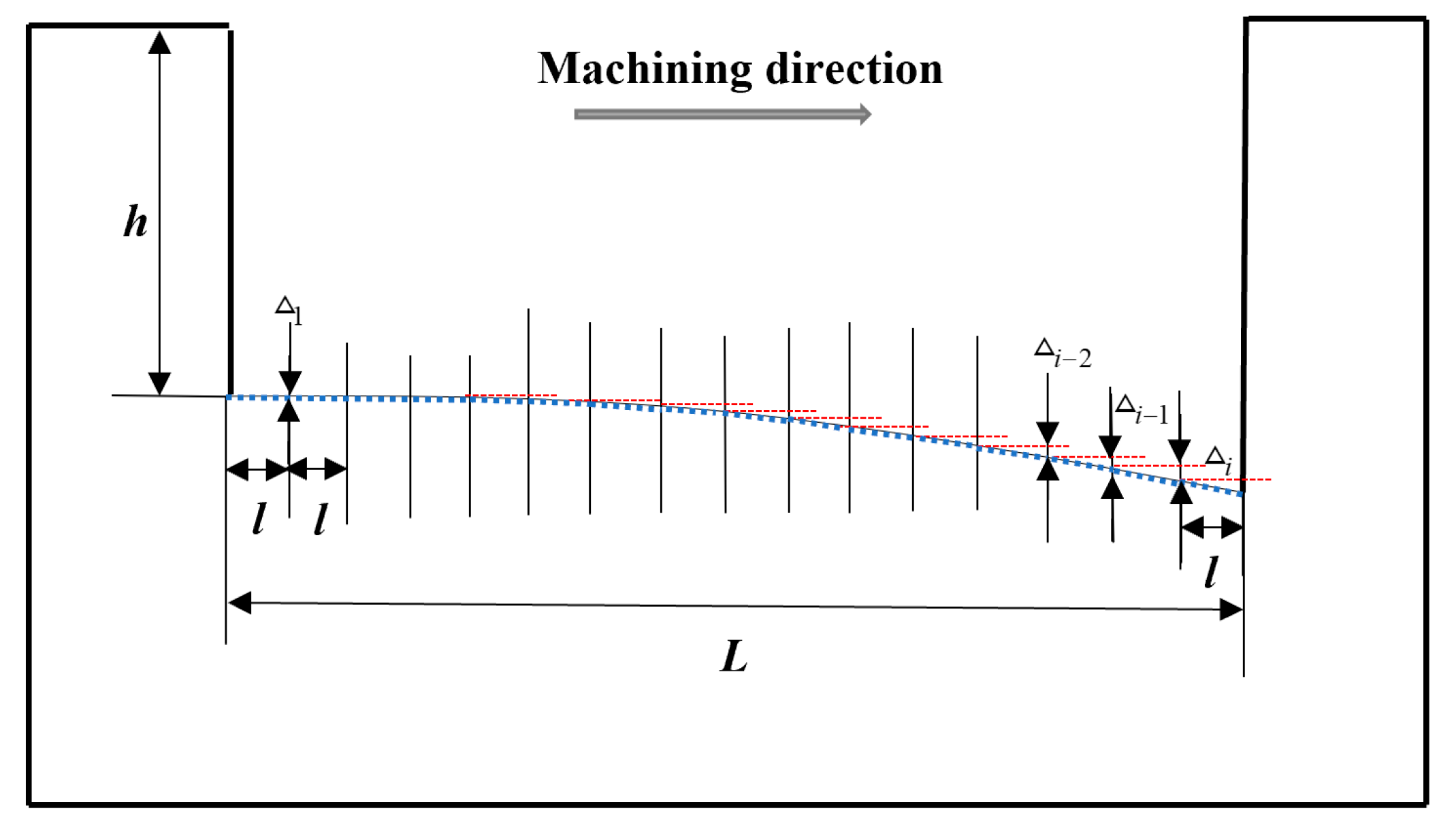
4.3. Compensation Machining
5. Conclusions
- Through orthogonal experiment design and analysis, the influence of machining parameters on machining performance can be obtained. The influence of Ip, Up, and fp on machining time is significantly greater than that of wp and Rot. The influence of the non-electrical factor Rot on electrode axial and radial wear is significantly smaller than that of the electrical factors Ip, Up, fp and wp.
- The GRA method is used to optimize machining performance at the same time. The optimized combination of factor levels is Ip = 30 Index, Up = 100 V, fp = 120 kHz, wp = 4 μs, and Rot = 700 rpm. The machining time required for microgroove micro-EDM is 50.28 s, electrode axial wear is 152.29 μm, and electrode radial wear is 55.52 μm. Compared to the H17 orthogonal experiment, the machining time is shortened by 10.01%, electrode axial wear is reduced by 2.02%, and electrode radial wear is reduced by 10.80%.
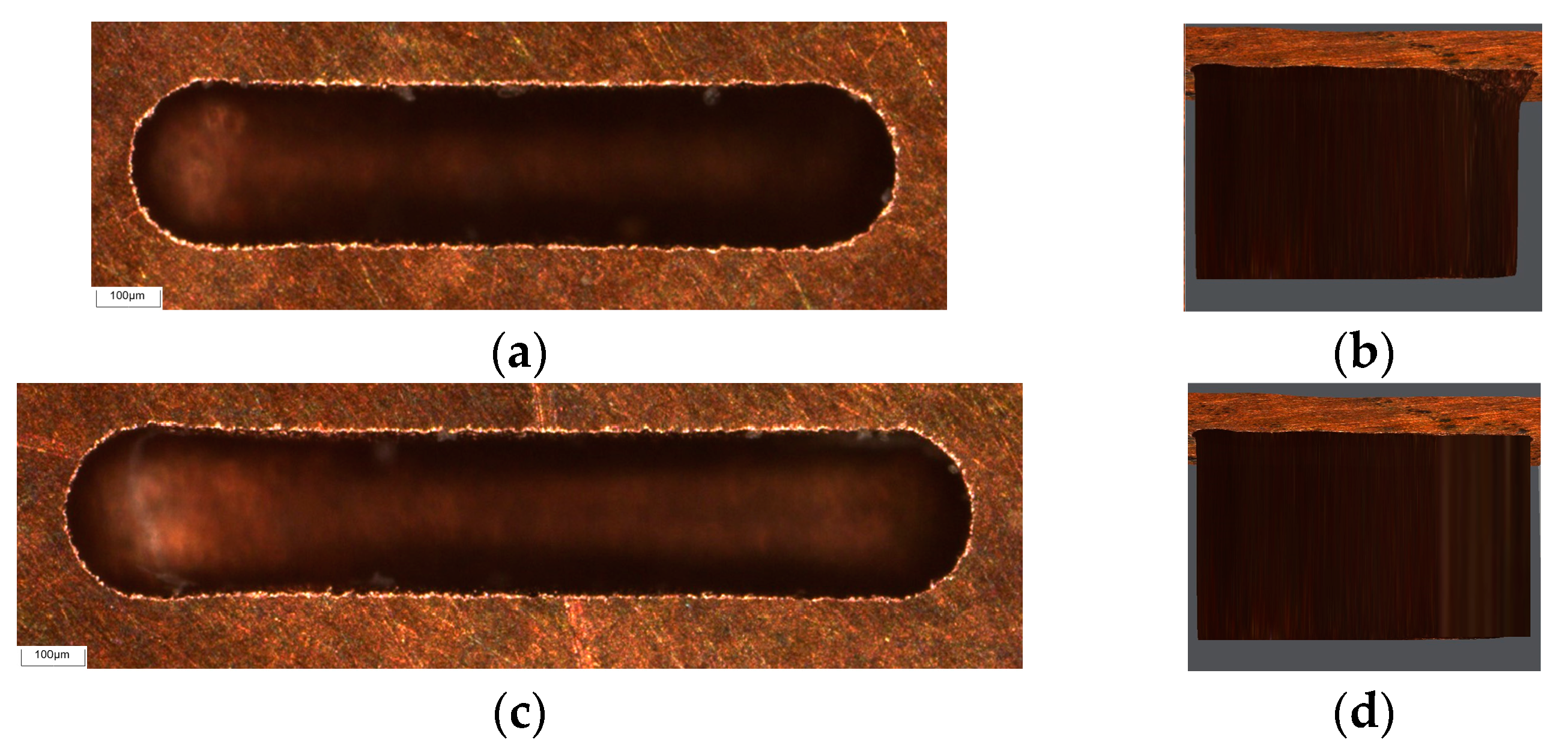
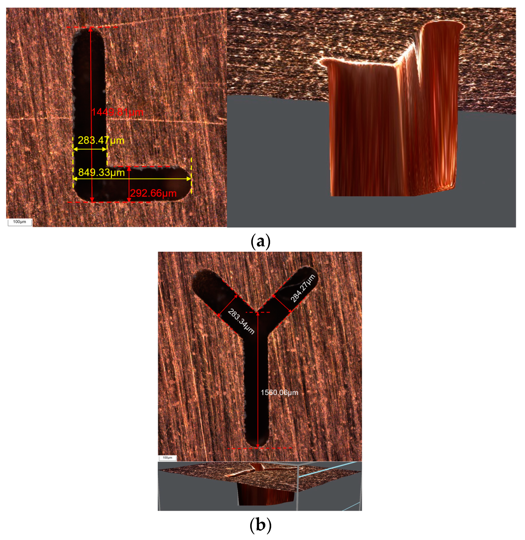
- Compared to microgroove machined without compensation under the GRA optimization factors combination, the fixed-length nonlinear compensation method proposed in this paper is used to compensate for electrode axial wear during machining. As a result, microgroove morphology with good consistency of depth and width is machined, which improves the machining quality of microgroove. It also shows that the compensation method has certain compensation accuracy and feasibility.
Author Contributions
Funding
Data Availability Statement
Conflicts of Interest
Abbreviations
| EDM | Electric discharge machining |
| ANN | Artificial neural network |
References
- Wang, P.; Bai, Q. The modelling and analysis of micro-milling forces for fabricating thin-walled micro-parts considering machining dynamics. Machines 2022, 10, 217. [Google Scholar] [CrossRef]
- Lin, W.; Fan, F. Analysis of the warpage phenomenon of micro-sized parts with precision injection molding by experiment, numerical simulation, and grey theory. Polymers 2022, 14, 1845. [Google Scholar] [CrossRef] [PubMed]
- Mouralova, K.; Bednar, J. Production of precision slots in copper foil using micro EDM. Sci. Rep. 2022, 12, 5023. [Google Scholar] [CrossRef]
- Zhang, H.; Wang, X. Formability and mechanism of pulsed current pretreatment-assisted laser impact micro-forming. J. Adv. Manuf. Technol. 2021, 114, 1011–1029. [Google Scholar] [CrossRef]
- Hu, Y.; Qi, H. Topologically devised flexible bi-aeolotropic conduction Janus-like bi-layer membrane functionalized by red-green bicolor fluorescence. J. Mater. Res. Technol. 2023, 24, 8644–8655. [Google Scholar] [CrossRef]
- Wang, J.; Yang, M. Ventilation condition effects on heat dissipation of the lithium-ion battery energy storage cabin fire. Case Stud. Therm. Eng. 2024, 63, 105373. [Google Scholar] [CrossRef]
- Anwar, S.; Rasool, G. Impact of Viscous Dissipation and Ohmic Heating on Natural Convection Heat Transfer in Thermo-Magneto Generated Plume. Front. Heat Mass Transf. 2024, 22, 1323–1341. [Google Scholar] [CrossRef]
- Zhang, S.; Shi, H. Research on the Milling Performance of Micro-Groove Ball End Mills for Titanium Alloys. Lubricants 2024, 12, 204. [Google Scholar] [CrossRef]
- Cao, Z.-H.; Tang, J. Full Cross-Sectional Profile Measurement of a High-Aspect-Ratio Micro-Groove Using a Deflection Probe Measuring System. Sensors 2025, 25, 2335. [Google Scholar] [CrossRef]
- Peng, Z.; Feng, T. Directly writing patterning of conductive material by high voltage induced weak electric arc machining (HV-μEAM). Coatings 2019, 9, 538. [Google Scholar] [CrossRef]
- Zhuang, W.H. Research on Microfine EDM Method for Strip Electrodes with Microchannel Structure; Xiamen University: Xiamen, China, 2021. [Google Scholar] [CrossRef]
- Bissacco, G.; Tristo, G. Uncertainty of the electrode wear on-machine measurements in micro-EDM milling. J. Manuf. Process. 2021, 64, 153–160. [Google Scholar]
- Mahbub, M.R.; Rashid, A. Strategies of improving accuracy in micro-EDM. In Micro Electro-Fabrication; Elsevier: Amsterdam, The Netherlands, 2021; pp. 159–194. [Google Scholar]
- Tong, H.; Li, Y. Servo scanning 3D micro EDM for array micro cavities using on-machine fabricated tool electrodes. J. Micromechan. Microeng. 2018, 28, 025013. [Google Scholar] [CrossRef]
- Sharma, A. Zero Wear Electrode for EDM Using Electrically Conductive Diamond. Ph.D. Thesis, Report of Researches, Nippon Institute of Technology, Saitama, Japan, 2006. Volume 36. pp. 33–40. [Google Scholar]
- Yu, Z.Y.; Masuzawa, T. Micro-EDM for three-dimensional cavities-development of uniform wear method. CIRP Ann. 1998, 47, 169–172. [Google Scholar] [CrossRef]
- Aliyu, A.A.; Rohani, J.M. Optimization of electrical discharge machining parameters of Si/SiC through response surface methodology. J. Technol. 2017, 79, 119–129. [Google Scholar]
- Kaneko, T.; Tsuchiya, M. Improvement of 3D NC contouring EDM using cylindrical electrode-optical measurement of electrode deformation and machining of free-curves. In Proceedings of the 10th International Symposium for Electro Machining (ISEM-X), Magdeburg, Germany, 6–8 May 1992; pp. 364–367. [Google Scholar]
- Yu, Z.Y.; Rajurkar, K.P. Study of 3D micro-ultrasonic machining. J. Manuf. Sci. Eng. 2004, 126, 727–732. [Google Scholar] [CrossRef]
- Yu, Z.Y.; Kozak, J. Modelling and simulation of micro EDM process. CIRP Ann. 2003, 52, 143–146. [Google Scholar] [CrossRef]
- Hang, G.R.; Cao, G.H. Micro-EDM milling of micro platinum hemisphere. In Proceedings of the 1st IEEE International Conference on Nano/Micro Engineered and Molecular Systems, Zhuhai, China, 19–21 January 2006; pp. 579–584. [Google Scholar]
- Gou, J.; Lai, J. Fabrication of high accuracy micro-hole by micro-EDM under tool electrode spiral motion feed mode aided with fixed reference axial compensation. Res. Sq. 2022. [Google Scholar] [CrossRef]
- Karmiris, P. Multiphysics Thermo-fluid Modeling and Experimental Validation of Crater Formation and Rim Development in EDM of Inconel C-276. Simul. Model. Pract. Theory 2025, 141, 103097. [Google Scholar] [CrossRef]
- Zhong, M.; Yu, H. Optimization of heat treatment process parameters for GH4738 superalloy based on Taguchi-Grey relational analysis method. Mater. Lett. 2025, 387, 138240. [Google Scholar] [CrossRef]
- Winarso, R.; Slamet, S. Optimization of 3D Printed Voronoi Microarchitecture Bone Scaffold using Taguchi-Grey Relational Analysis. Bioprinting 2025, 47, e00402. [Google Scholar] [CrossRef]
- Xu, J.K.; Li, M.Y. Process Parameter Modeling and Multi-Response Optimization of Wire Electrical Discharge Machining NiTi Shape Memory Alloy. Mater. Today Commun. 2022, 33, 104252. [Google Scholar] [CrossRef]
- Richard, S.P.; Titus, S. Efficient energy management using Red Tailed Hawk optimized ANN for PV, battery & super capacitor driven electric vehicle. J. Energy Storage 2025, 117, 116126. [Google Scholar]
- Wang, Y.Z. Detection of lane line based on Robert operator. JME 2021, 9, 156–166. [Google Scholar]
- Wang, Y.; Yin, T. A steel defect detection method based on edge feature extraction via the Sobel operator. Sci. Rep. 2024, 14, 27694. [Google Scholar] [CrossRef]
- Tenekeci, M.; Abdulazeez, S.T. Edge detection using the Prewitt operator with fractional order telegraph partial differential equations (PreFOTPDE). In Multimedia Tools and Applications; Springer: Berlin/Heidelberg, Germany, 2024; pp. 1–17. [Google Scholar]
- Su, Z.Y.; Zhang, W.H. Quantum image edge detection based on Laplacian of Gaussian operator. Quantum Inf. Process. 2024, 23, 178. [Google Scholar]
- Ma, P.; Yuan, H. A Laplace operator-based active contour model with improved image edge detection performance. Digit. Signal Process. 2024, 151, 151104550. [Google Scholar] [CrossRef]
- Gaurak; Ghanekar, U. Image steganography based on canny edge detection, dilation operator and hybrid coding. J. Inf. Secur. Appl. 2018, 41, 41–51. [Google Scholar]
- Zhang, M.; Guo, H. Compensation method of wire electrode wear for reciprocating micro wire electrical discharge machining. J. Manuf. Process. 2023, 86, 136–142. [Google Scholar] [CrossRef]
- Zhang, X.D.; Li, Y.Q. High-quality and efficiency machining of micro-EDM. In Proceedings of the 2024 IEEE International Conference on Manipulation, Manufacturing and Measurement on Nanoscale (3M NANO), Gijon, Spain, 8–11 July 2024; IEEE: Piscataway, NJ, USA, 2024; pp. 105–110. [Google Scholar]


| Density (g/cm3) | Melting Point (°C) | Poisson’s Ratio | Specific Heat Capacity (J/kg×K) | Modulus of Elasticity (GPa) | Thermal Conductivity (W/m×K) |
|---|---|---|---|---|---|
| 8.96 | 1083 | 0.33 | 385 | 100–110 | 401 |
| Dielectric Constant | Insulation Strength (mv/m) | Density (Kg/m3) | Stickiness (mm2/s) | Combustion Point (°C) | Flash Point (°C) |
|---|---|---|---|---|---|
| 3 | 14–22 | 813 | 7.0 | 243 | 134 |
| Level | Ip (A) | Up (V) | fp (kHz) | Rot (rpm) | wp (μs) |
|---|---|---|---|---|---|
| 1 | 25 | 90 | 110 | 600 | 3 |
| 2 | 30 | 100 | 120 | 700 | 4 |
| 3 | 35 | 110 | 130 | 800 | 5 |
| Number | Ip (A) | Up (V) | fp (kHz) | Rot (rpm) | wp (μs) |
|---|---|---|---|---|---|
| H1 | 1(25) | 1(100) | 1(110) | 1(600) | 1(2) |
| H2 | 1 | 1 | 1 | 1 | 2(3) |
| H3 | 1 | 1 | 1 | 1 | 3(4) |
| H4 | 1 | 2(110) | 2(120) | 2(700) | 1 |
| H5 | 1 | 2 | 2 | 2 | 2 |
| H6 | 1 | 2 | 2 | 2 | 3 |
| H7 | 1 | 3(120) | 3(130) | 3(800) | 1 |
| H8 | 1 | 3 | 3 | 3 | 2 |
| H9 | 1 | 3 | 3 | 3 | 3 |
| H10 | 2(30) | 1 | 2 | 3 | 1 |
| H11 | 2 | 1 | 2 | 3 | 2 |
| H12 | 2 | 1 | 2 | 3 | 3 |
| H13 | 2 | 2 | 3 | 1 | 1 |
| H14 | 2 | 2 | 3 | 1 | 2 |
| H15 | 2 | 2 | 3 | 1 | 3 |
| H16 | 2 | 3 | 1 | 2 | 1 |
| H17 | 2 | 3 | 1 | 2 | 2 |
| H18 | 2 | 3 | 1 | 2 | 3 |
| H19 | 3(35) | 1 | 3 | 2 | 1 |
| H20 | 3 | 1 | 3 | 2 | 2 |
| H21 | 3 | 1 | 3 | 2 | 3 |
| H22 | 3 | 2 | 1 | 3 | 1 |
| H23 | 3 | 2 | 1 | 3 | 2 |
| H24 | 3 | 2 | 1 | 3 | 3 |
| H25 | 3 | 3 | 2 | 1 | 1 |
| H26 | 3 | 3 | 2 | 1 | 2 |
| H27 | 3 | 3 | 2 | 1 | 3 |
| Number | Machining Time | Axial Electrode Wear | Radial Electrode Wear | Grey Relational Grade | Rank |
|---|---|---|---|---|---|
| 1 | 0.683774 | 0.355223 | 0.422137 | 0.487045 | 26 |
| 2 | 0.535804 | 0.410972 | 0.465554 | 0.470777 | 27 |
| 3 | 0.7 | 0.504785 | 0.46019 | 0.554991 | 22 |
| 4 | 0.620897 | 0.618066 | 0.605628 | 0.614864 | 12 |
| 5 | 0.565995 | 0.78091 | 0.733858 | 0.693588 | 2 |
| 6 | 0.494982 | 0.777784 | 0.667543 | 0.64677 | 5 |
| 7 | 0.601902 | 0.549356 | 0.733333 | 0.628197 | 6 |
| 8 | 0.451408 | 0.549321 | 0.5 | 0.500243 | 25 |
| 9 | 0.617012 | 0.502239 | 0.50976 | 0.543004 | 24 |
| 10 | 0.582181 | 0.673715 | 0.612959 | 0.622952 | 9 |
| 11 | 0.530232 | 0.780498 | 0.566058 | 0.625596 | 7 |
| 12 | 0.564363 | 0.870667 | 0.534302 | 0.656444 | 4 |
| 13 | 0.567464 | 0.683463 | 0.613082 | 0.621336 | 10 |
| 14 | 0.666667 | 0.636953 | 0.568709 | 0.624109 | 8 |
| 15 | 0.63688 | 0.584366 | 0.641194 | 0.620813 | 11 |
| 16 | 0.58254 | 0.729469 | 0.666069 | 0.65936 | 3 |
| 17 | 0.557034 | 0.81637 | 0.750316 | 0.707907 | 1 |
| 18 | 0.564913 | 0.645772 | 0.625597 | 0.612094 | 13 |
| 19 | 0.531063 | 0.632498 | 0.559871 | 0.574477 | 19 |
| 20 | 0.509877 | 0.590246 | 0.615013 | 0.571712 | 20 |
| 21 | 0.563142 | 0.554741 | 0.6447 | 0.587528 | 18 |
| 22 | 0.60052 | 0.647126 | 0.578038 | 0.608561 | 14 |
| 23 | 0.53989 | 0.614634 | 0.648712 | 0.601079 | 16 |
| 24 | 0.560445 | 0.547922 | 0.592146 | 0.566837 | 21 |
| 25 | 0.622941 | 0.625676 | 0.569308 | 0.605975 | 15 |
| 26 | 0.554208 | 0.584631 | 0.656491 | 0.598443 | 17 |
| 27 | 0.528305 | 0.549103 | 0.572383 | 0.54993 | 23 |
| Level | Ip | Up | fp | wp | Rot |
|---|---|---|---|---|---|
| 1 | 0.567866 | 0.576936 | 0.557011 | 0.574984 | 0.634855 |
| 2 | 0.715842 | 0.698822 | 0.72796 | 0.635448 | 0.718579 |
| 3 | 0.496075 | 0.520651 | 0.509786 | 0.596781 | 0.530551 |
| Range | 0.219768 | 0.178171 | 0.218173 | 0.060464 | 0.188028 |
| Nonlinear Functions | R2 | Adj R2 | RMSE |
|---|---|---|---|
| 0.9943 | 0.9924 | 0.0080 | |
| 0.9719 | 0.9625 | 1.5742 | |
| 0.9853 | 0.9706 | 1.3936 |
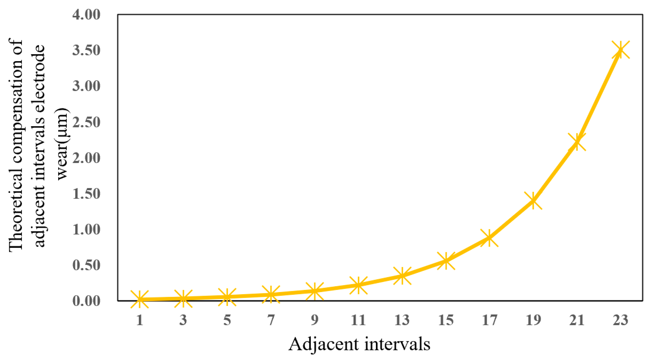
| Number of Intervals | Theoretical Compensation (μm) | Electrode Wear During Compensation (μm) | Actual Compensation (μm) |
|---|---|---|---|
| 1 | 0.0223 | 0.0045 | 0.0268 |
| 3 | 0.0354 | 0.0071 | 0.0425 |
| 5 | 0.0559 | 0.0112 | 0.0671 |
| 7 | 0.0886 | 0.0230 | 0.1116 |
| 9 | 0.1403 | 0.0365 | 0.1768 |
| 11 | 0.2223 | 0.0667 | 0.2890 |
| 13 | 0.3522 | 0.1127 | 0.4649 |
| 15 | 0.5579 | 0.1897 | 0.7476 |
| 17 | 0.8838 | 0.3182 | 1.2020 |
| 19 | 1.4000 | 0.5880 | 1.9880 |
| 21 | 2.2177 | 0.9980 | 3.2157 |
| 23 | 3.5129 | 1.6862 | 5.1991 |
Disclaimer/Publisher’s Note: The statements, opinions and data contained in all publications are solely those of the individual author(s) and contributor(s) and not of MDPI and/or the editor(s). MDPI and/or the editor(s) disclaim responsibility for any injury to people or property resulting from any ideas, methods, instructions or products referred to in the content. |
© 2025 by the authors. Licensee MDPI, Basel, Switzerland. This article is an open access article distributed under the terms and conditions of the Creative Commons Attribution (CC BY) license (https://creativecommons.org/licenses/by/4.0/).
Share and Cite
Zhang, X.; Zhang, W.; Yu, P.; Li, Y. Research on Machining Parameter Optimization and an Electrode Wear Compensation Method of Microgroove Micro-EDM. Micromachines 2025, 16, 481. https://doi.org/10.3390/mi16040481
Zhang X, Zhang W, Yu P, Li Y. Research on Machining Parameter Optimization and an Electrode Wear Compensation Method of Microgroove Micro-EDM. Micromachines. 2025; 16(4):481. https://doi.org/10.3390/mi16040481
Chicago/Turabian StyleZhang, Xiaodong, Wentong Zhang, Peng Yu, and Yiquan Li. 2025. "Research on Machining Parameter Optimization and an Electrode Wear Compensation Method of Microgroove Micro-EDM" Micromachines 16, no. 4: 481. https://doi.org/10.3390/mi16040481
APA StyleZhang, X., Zhang, W., Yu, P., & Li, Y. (2025). Research on Machining Parameter Optimization and an Electrode Wear Compensation Method of Microgroove Micro-EDM. Micromachines, 16(4), 481. https://doi.org/10.3390/mi16040481