Article

Performance Characterization of Micromachined Inductive Suspensions Based on 3D Wire-Bonded Microcoils

Laboratory for Microactuators, Department of Microsystems Engineering—IMTEK, University of Freiburg, Georges-Koehler-Allee 102, D-79110 Freiburg, Germany
*
Author to whom correspondence should be addressed.
Micromachines 2014, 5(4), 1469-1484; https://doi.org/10.3390/mi5041469
Submission received: 30 September 2014 / Revised: 1 December 2014 / Accepted: 5 December 2014 / Published: 12 December 2014
(This article belongs to the Special Issue Microactuators)

Abstract

:
We present a comprehensive experimental investigation of a micromachined inductive suspension (MIS) based on 3D wire-bonded microcoils. A theoretical model has been developed to predict the levitation height of the disc-shaped proof mass (PM), which has good agreement with the experimental results. The 3D MIS consists of two coaxial wire-bonded coils, the inner coil being used for levitation, while the outer coil for the stabilization of the PM. The levitation behavior is mapped with respect to the input parameters of the excitation currents applied to the levitation and stabilization coil, respectively: amplitude and frequency. At the same time, the levitation is investigated with respect to various thickness values (12.5 to 50 μm) and two materials (Al and Cu) of the proof mass. An important characteristic of an MIS, which determines its suitability for various applications, such as, e.g., micro-motors, is the dynamics in the lateral direction. We experimentally study the lateral stabilization force acting on the PM as a function of the linear displacement. The analysis of this dependency allows us to define a transition between stable and unstable levitation behavior. From an energetic point of view, this transition corresponds to the local maximum of the MIS potential energy. 2D simulations of the potential energy help us predict the location of this maximum, which is proven to be in good agreement with the experiment. Additionally, we map the temperature distribution for the coils, as well as for the PM levitated at 120 μm, which confirms the significant reduction of the heat dissipation in the MIS based on 3D microcoils compared to the planar topology.

Graphical Abstract

1. Introduction

Magnetic levitation is a non-contact process to suspend an object stably against gravity using various magnetic interaction principles. With the tremendous development of microfabrication technologies and the emergence of the MEMS (micro-electro-mechanical systems) field, a plethora of magnetic levitation applications at the micro-scale have been reported in a wide variety of domains, such as cell culturing [1], micro-manipulation [2] or micro-bearings [3].
Amongst various magnetic levitation principles, we will focus our attention on inductive levitation, as it exploits the eddy currents induced in an electrically-conductive and non-magnetic proof mass (PM) in order to generate a repulsive force that levitates the PM. Inductive levitation in conjunction with microfabrication techniques has the advantage of operating without permanent micromagnets, which are otherwise difficult to implement and, in spite of notable recent efforts in the field [46], are still rather incompatible with MEMS technology.
The first micromachined inductive suspension (MIS) prototype was demonstrated in 1995 by Shearwood et al. exclusively using planar microfabrication techniques (2D) [7]. A 400 μm diameter Al PM of 12 μm thickness was levitated at a height of 30 μm with a current root mean square (RMS) value of 600 mA at 10 MHz using planar microcoils. A micro-gyroscope based on this prototype was demonstrated five years later [8] employing three different coils for levitation, stabilization and rotation, respectively, all of them integrated as one single planar structure. A second input signal was superimposed on the coil for PM rotation. Furthermore, the temperatures of the PM and the coil at a 350 mA RMS current were measured to be 50 °C and 600 °C, respectively.
One step forward has been achieved by Wu et al. by separating the rotation and stabilization/levitation coils, in order to gain more freedom and separate AC (alternative current) signals with different frequencies and their corresponding electromagnetic fields [9]. Capacitive displacement sensing has been also introduced by additional electrodes to sense the change of capacitance between electrodes and PM. However, these achievements have been obtained at the expense of a significant increase in the fabrication complexity. Four additional lithography levels have been introduced to obtain two separate metal layers and for the electroplating of 16 coils and 32 contacts. The levitation height was 20 μm for an Al PM with a 2000 μm diameter and a 20 μm thickness, using a current amplitude of 300 mA at 10 MHz according to simulation results.
Very recently, Sari and Kraft have introduced a new element in the micromachined inductive suspensions: linear movement. They presented a micro-accelerator based on induction levitation, which only requires a two-mask fabrication process [10]. The PM was propelled along a pre-defined linear track by an electrostatic force. Still, a current of 0.6 A at 45 MHz was used to levitate the 7 μm thick Al PM to 85 μm.
All devices presented above share a common point: the usage of planar coils for MIS. The planar coil technology imposes severe restrictions in the number of metal layers needed either for separating the coils with different functionalities, e.g., levitation, stabilization and rotation, or for the total number of windings available to generate the excitation variable magnetic field. Each additional metal layer introduces several additional masks for metallization, etching, electroplating, passivation and vias. In order to compensate for this, large currents are needed, leading to high temperatures in the substrate, potential stress and delamination of the electroplated metal and eventually device failure.
We focus our efforts in the MIS field on the usage of three-dimensional (3D) microcoils. As opposed to their 2D counterparts, 3D coils provide more concentrated and uniform magnetic fields, as well as a larger number of windings. We have reported the preliminary results of a 3D MIS based on the combination of wire bonding and microfabrication techniques [11,12]. Only two masks were needed for fabrication: one for the metal layer serving as contact pads, the other to define the mechanical support structures of the 3D wire-bonded micro-coils. An Al disc of 25 μm in thickness and 3200 μm in diameter was levitated up to 150 μm at a 2 MHz excitation signal with 105 mA RMS current for both levitation and stabilization coils. The number of windings of the 3D wire bonded coil is dramatically increased, which allows us to use lower current values due to the larger ampere-turn value. This coil with a significantly increased number of windings is fabricated in one single step, which would equivalate with tens of additional process steps (lithography, metallization, etching, electroplating and passivation) using only planar techniques.
Very recently, we have reported an analytical model to predict the behavior of the levitated PM from the point of view of stability [13]. We have mapped the stability levitation domains, and we have analytically found and experimentally verified the values corresponding to vertical, lateral and angular stiffness, respectively.
In this paper, we focus on the characterization of the 3D MIS with respect to the input parameters: the amplitude and the frequency of the currents in the levitation and stabilization coil, respectively. Section 2 of the paper reviews the MIS operating principle along with design considerations specific to 3D MIS. The effects of 3D coils with one or two layers of windings are discussed. Section 3 presents the experimental setup and studies the levitation height for various thickness values of the PM and for two different materials: copper and aluminum. We provide a comprehensive map of the levitation height as a function of the amplitude of the two input currents, revealing the stable levitation domain. Accounting for the effect of frequency, a theoretical model has been developed to predict the levitation height of the proof mass. Lateral stability is experimentally studied as an important parameter that defines the potential usefulness of the MIS in applications, such as micro-motors, and heat dissipation is estimated and compared to the case of 2D MIS structures. Section 4 concludes with a discussion and prospects about 3D MIS.

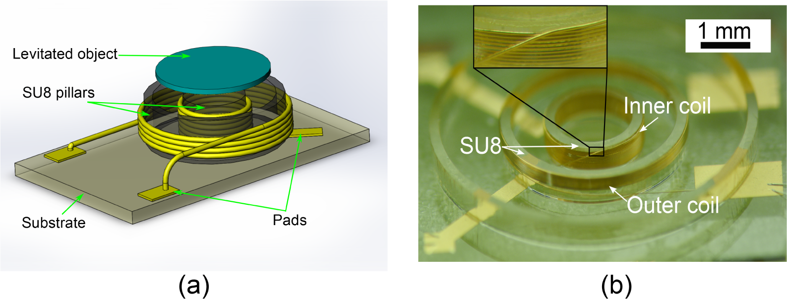
2. Mechanism and Design

2.1. Operating Principle

The operating principle has been described in detail in the previous work from Shearwood [8], as well as in our own earlier contribution [11]. Briefly, the 3D MIS consists of two coaxial wire bonded coils, as shown in Figure 1. Each coil is fed with an AC current, the phase shift between the two currents being 180°. Eddy currents are induced in the conductive disk-shaped PM, which is levitated above the coils due to the interactions between the input and eddy currents. In this configuration, the inner coil is responsible for the levitation effect, while the outer coil is responsible for the stabilization of the PM. The PM is levitated at the equilibrium position by the Lorentz force. The equilibrium position of the levitated PM is where levitation force (Flev, total Lorentz force in vertical direction over the levitating PM) equals the weight of the PM:
G pm = F lev = Ω B r ( r , z , ω ) i φ ( r , z , ω ) d l
where Gpm is the weight of the PM, Ω is the volume of the PM, Br is the radial component of magnetic flux densities generated by input currents, iφ is the φ-component of eddy currents, ω is the frequency of the excitation signal and dl is an infinitesimal path of the PM where iφ goes. The PM oscillates along or about any axis near the equilibrium position. As we have reported in [13], the PM can be approximately treated as a harmonic oscillator, with “elastic constants” corresponding to stiffness values in three orientations: vertical, lateral and angular.

2.2. Coil Impedance and Design

The major advantage of 3D wire-bonded coils used in this work, compared with 2D coils, is the easiness of obtaining a relatively large number of windings, thus a significantly larger ampere-turn value. In order to achieve a larger upward vertical component of the Lorentz force, therefore a larger levitation effect, the number of windings of the inner (levitation) coil, should be increased. The parameters of the outer (stabilization) coil, such as position, diameter, number of windings and current intensity, contribute to the stabilization of the proof mass and are reflected in the stiffness of the structure, as shown in [13]. We have previously thoroughly explained the wire bonding process used in the fabrication of the 3D solenoidal coils [14]. Basically, the movement of the head of an automatic wire bonder is controlled via a MATLAB interface where a three-dimensional helical trajectory is defined. The head of the wire bonder moves according to the defined trajectory around a pillar structured in thick SU-8 using UV lithography. The wire plastically deforms to the shape of the SU-8 pillar remaining as a solenoidal 3D coil. In this work, the typical height of the SU-8 pillars was 650 μm, and there is no pitch between adjacent wires. The wire used here is insulated gold wire, 25 μm in diameter.
In our design shown in Figure 1, two aspects have been considered. The first aspect is the operation range of the device, which should be well below the resonant frequency of the coils. When the frequency of excitation currents gets close to the resonant frequency, the coil impedance increases dramatically, making the MIS hard to drive. The second aspect is that the two coils should have similar impedance values for the easiness of operation and control and without reducing the generality of the experiments.
The resonant frequency of the coil, f0, is defined by:
f 0 = 1 2 π 1 L C ( R L ) 2
where L, C and R are the inductance, stray capacitance and resistance of the coil, respectively. In the case of single-layer 3D microcoils, the inductance is very well approximated by Wheeler’s formula [15]:
L = 10 π μ 0 N 2 r 2 9 r + 10 h c o i l = 10 π μ 0 N 2 r 2 9 r + 10 N p
where μ0 is the vacuum permeability, N is the number of windings, r is the coil radius, hcoil is the coil height and p is the pitch between two adjacent windings and, in our particular case, p is equal to the wire diameter. Even though 3D coils have larger hcoil, by rewriting hcoil as Np in Equation (3), it can be assumed that L is proportional to N. Therefore, when employing 3D microcoils, the inductance values are much larger than in the case of 2D microcoils. The stray capacitance also increases significantly because the wires are adjacent to each other. As a consequence, following from Equation (2), resonant frequencies of the 3D coils composing the micromachined inductive suspensions are much lower compared to the 2D case. This is another important difference that needs to be taken into account when employing 3D MIS with respect to their 2D counterparts.
The algorithm proposed in [16] is used for the calculation of self- and mutual inductances of coaxial current coils over the whole range of coil sizes and shapes, being fast and accurate. As the material properties and the thickness of the wire insulation layer are not disclosed due to commercial interest, we could only roughly estimate the stray capacitance of the coils using the method in [17], thus the resonant frequency. When the inner coil has a diameter of 2000 μm and 20 windings arranged in one layer, the calculated self-inductance was 1.19 μH, while the stray capacitance value was 2.19 pF. Therefore, the coil inductance is the dominant factor for coil impedance. In order to obtain the same inductance, the outer coil should have 12 windings arranged in one layer for a diameter of 3900 μm. The diameter difference between the two coils comes from the SU-8 sidewall thickness and the minimum requirement of post-capillary distance in the wire bonding process (400 μm), which determines a minimum diameter difference between the outer and inner coil. In this work, the number of winding layers was set to 1, so that a large tuning range of both input current amplitude and frequency was possible for experimental characterization purposes. The detailed fabrication process can also be found in [13].
In order to verify our assumptions and the theoretical calculations and to determine the MIS working frequency range, we measured the impedances of inner and outer coils using an impedance analyzer, Agilent 4991A (Agilent Technologies, Santa Clara, CA, USA). The results are shown in Figure 2. The inductance of the single-layer coil far left from the resonant frequency was measured to be 1.16 μH, with the resonant frequency of 111 MHz. The inductance of the 2D MIS in [8] with the same size in diameter was only about 10 nH and a resonant frequency of 15 GHz according to simulations carried out with Agilent Advanced Design Systems. The repeatability of coil electrical parameters for single-layer coils was reported to be excellent in [5].
For comparison, Figure 2b also includes the impedance of coils having twice the number of windings arranged in two layers, showing that the resonant frequency for these structures drops almost four times compared to the one-layer structures. This proves that the potential working frequency range is further drastically reduced in double-layer coils.

3. Characterization

In the following subsections, we present a complete performance characterization of the 3D MIS. After introducing the experimental setup, a complete mapping of performance vs. operational conditions in terms of current amplitudes and frequencies is shown, as well as a stability analysis and considerations about the heat dissipation in the device.

3.1. Experimental Setup

The experimental setup for performance characterization is shown in Figure 3a. The computer controlled function generator (Arbstudio 1104D, Lecroy, Chestnut Ridge, NY, USA) generated the excitation signal for each coil. We independently controlled the phase, amplitude and frequency of the two signals. Two amplifiers (A093R, LCF, Post Falls, ID, USA) were used to provide current-amplified signals to the MIS, which was fixed on an optical breadboard (UltraLight series, Thorlabs, Newton, NJ, USA) with vibration isolation feet. The current through each coil was observed by measuring the voltage signal using a Lecroy 64MXi oscilloscope (equipped with 9.5 pF probes) on a series resistor, which behaves like a pure resistor in our working frequency range. The levitation height was measured by an LK-G32 laser sensor (Keyence, Osaka, Japan). Compared to the preliminary results reported in [11], we extend here the study range of input currents in both amplitude and frequency, at the same time also exploring the stability of the 3D MIS. The mechanical properties to assess the stability of the PM were measured using a microforce sensing probe (FEMTO TOOLS AG, Buchs, Switzerland). The temperature of the device was measured by an IR (Infrared) camera PI-160 (Optris GmbH, Berlin, Germany).

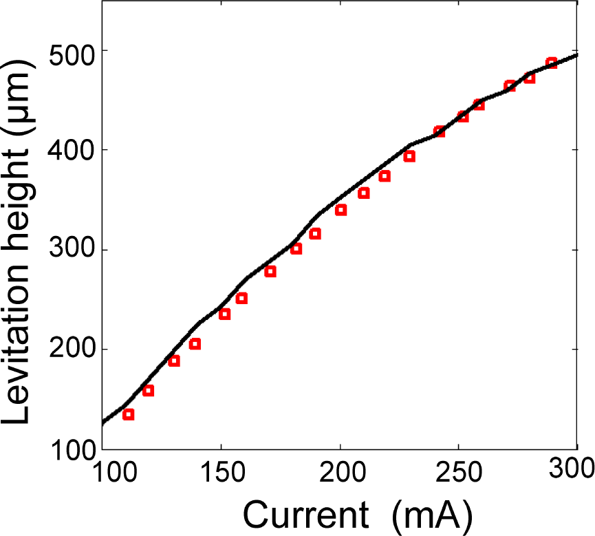
3.2. Control of Levitation Height

3.2.1. Levitation Height vs. Excitation Signal: Experimental

According to Faraday’s law, the electromotive force (EMF) induced in the PM is proportional to the rate of change of the excitation magnetic flux: the higher the frequency of the input current, the larger the EMF. Increasing the frequency, the skin depth effect becomes dominant, as has been experimentally reported for the 2D MIS in [8,9,18].
We study the dependency of the levitation height on the input current frequency for proof masses with various thicknesses, 13, 25 and 50 μm for aluminum and 12.5 μm for copper, and, therefore, different ratios of skin depth to thickness. These measurements have been performed with a 3D MIS structure having the inner (levitation) coil with a diameter of 2000 μm and 20 windings and the outer (stabilization) coil with a diameter of 3900 μm and 12 windings, which is denoted as MIS1 in Figure 4. Additionally, we studied another 3D MIS structure having a different number of windings for the inner (15 windings) and outer (9 windings) coils, respectively (MIS2). All measurements have been performed using a square wave excitation current in both inner and outer coils. The RMS values for the currents used in each experiment are indicated in Figure 4.
Figure 4 summarizes the experimental results showing the levitation height as a function of current frequency for constant RMS current values. From 2 to 8 MHz, the slopes of the curves corresponding to the PM with a thickness of 13 μm are steeper than the slopes of the curves corresponding to thicker PMs. Similarly, the slopes of the curves corresponding to 13 μm-thick Al PM are steeper than the curve for 12.5 μm-thick Cu PM. This verifies the expected effect of the skin depth, which is more obvious for thicker materials, as well as for materials with higher conductivities. At 4 MHz, the skin depth for aluminum is 41 μm and for copper is 32.6 μm, which means that the thinner PMs (12.5 and 13 μm) do not yet feel the skin effect, while this is already present for the thickest (50 μm) PM. A very important remark for these experiments is the fact that at higher frequencies, the square wave signal generated by the function generator gets distorted by the real characteristics of the circuit. A square wave signal of frequency f can be seen as a superposition of sine wave signals with frequency multiples of f, which will be amplified differently according to the gain vs. frequency curve of the amplifier. Therefore, at higher nominal frequencies of the input square wave, one will notice a mixture of phenomena arising from the fact that the coils composing the MIS structure are actually experiencing frequencies much closer to resonance, as well as mutual coupling effects between the coils and the proof mass, respectively. Since a thorough study of these phenomena exceeds the scope of the present paper, we only state the fact that for frequencies above 18 MHz, the skin effect takes over and the levitation height decreases with increasing the frequency.
The use of two amplifiers allows the independent study of the effects of the inner and outer coil. Figure 5 provides a map of the levitation height as a function of the inner coil and outer coil current RMS values. The levitation height is increased with the increase of the inner (levitation) coil current and is decreased with the increase of the outer (stabilization) coil current. This fact is in agreement with the general operation principle: the inner coil mainly contributes to the levitation effect, while the outer coil is responsible for the system stability. By referring to Figure 6, we find that the MIS showed good linear control of levitation height with respect to coil current. When the MIS is biased in the region characterized by large inner coil current and low outer coil current, the PM cannot be levitated stably, the so-called “unstable zone”. When the current in the outer coil is much larger than in the inner coil, the PM is stably tilted, as shown in Figure 5b. Moreover, as we have previously reported in [12], COMSOL simulation results of this special bias condition show that the Lorentz force is focused at the edge of the PM. This tilting of PM is due to the fact that the real MIS structure is asymmetric because of the spiral nature of the coils and the fact that the PM may not be perfectly flat and symmetrical. Any of these small asymmetries leads to the so-called “stably-tilted zone”.
In order to compare the levitation effects of 3D MIS to 2D MIS, we scaled up the 2D MIS reported in [8] to the same diameter of our 3D MIS. Using this scaled up 2D MIS, COMSOL simulation shows that it needs 12−times more input current compared to our 3D MIS (140 mA at 8 MHz) to levitate the same PM at the same height.

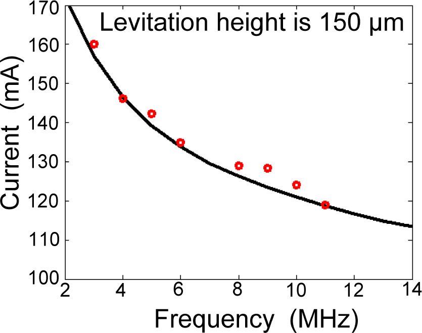
3.2.2. Theoretical Calculation of the Input Current and Frequency

Let us consider the equilibrium state of the micromachined inductive suspension in the vertical direction. As previously shown in [19], we can write:
m g + I 2 L PM L m l | l = h L m = 0
where m is the mass of PM, g is the gravitational acceleration, I is the current in the coils (assuming the same current in both coils), LPM is the self-induction of the PM and LPM is the mutual induction between the coils and the PM; in this particular case the mutual induction can be considered as a function of the PM vertical displacement, l. The equilibrium occurs at the point l = h, where h is the levitation height. The second term in Equation (4) represents the Ampère force acting between the coil and eddy currents and obtained as the derivative of the potential energy with respect to the vertical displacement.
The numerical analysis [12] shows that for a particular MIS design, the contribution of the levitation coil in the levitation force is significantly larger compared to the contribution of the stabilization coil. Additionally, the levitation coil induces the eddy current in the PM, the maximum value of which is distributed within a ring with the same radius as the levitation coil, as shown in [12]. Assuming that the levitation height of the proof mass is small and the fact that the function of mutual inductance between the disk-shaped proof mass and the ring-shaped coils can be simplified and expressed in terms of simple functions, the qualitative approach developed in [20] can be applied to the present study. Hence, the mutual induction can be represented in quadratic form as follows:
L m = c 0 + c l l + c u l 2
where c0, cl and cll are the coefficients of the quadratic form defined in equilibrium position (l = h). Static Equation (4) can be rewritten in terms of the coefficients of this quadratic form as follows:
m g I 2 c l ( h / α ( ω ) ) c 0 ( h / α ( ω ) ) L PM = 0
where α is an implicit function that takes into account the scaling effect of the excitation current frequency, ω, i.e., the increase of the maximum value of the eddy current with the increase of frequency. According to [13], the coefficients cl(h) and c0(h) can be defined as follows:
C 0 ( h ) = v = 0 M 1 r l μ 0 [ ln 8 r l ( h + v · p ) 1.92 ] ; c l ( h ) = v = 0 M 1 r l μ 0 ( h + v · p )
where M is the number of turns of the levitation coil, rl is the radius of the levitation coil and p is the pitch between consecutive windings of the coil. The self-induction of the ring-shaped path of the eddy current is defined as:
L PM = r l μ 0 [ ln 8 r l δ ( ω ) 0.3 ]
where δ is a frequency-dependent function whose physical meaning is the effective width in which the maximum of the induced eddy current within the PM is distributed. This dependency is a result of changing the sharpness of the distribution of the eddy current with frequency. As shown in [12], the effective width can be evaluated as δ = 0.01..0.1 · rl.
In this section, we will demonstrate that we can use the fundamental Equation (6), together with the parameters defined by δ(ω) and α(ω), to completely determine the state of the device, i.e., levitation height, input current and frequency. Figure 6 shows that a set of experimental data points (the red square points) representing levitation height versus excitation current in the levitation coil can be fitted with the theoretical curve generated by Equation (6) (the black line) for two properly chosen values for δ(ω) and α(ω). The measurement was carried out for a PM with a radius of 1.6 mm and a thickness of 13 μm, which was levitated by a levitation coil with a radius of 1 mm and 15 windings, fed by AC current with a frequency of 10 MHz. The fitting by Equation (6) was performed assuming that δ = 20 μm and α = 0.80.
Both functions, namely δ(ω) and α(ω), can be defined experimentally for a particular range of frequencies in a manner similar to the measurement and fitting presented in Figure 6. The measurements should be conducted for different reference points within the desired range of frequencies. For instance, in the case of a PM with a thickness of 13 μm and a levitation coil with a radius of 1 mm and 20 windings, we define the curves of α(ω) and δ(ω) within the frequency range from 2 to 14 MHz. We used four arbitrary reference points at 3, 6, 8 and 12 MHz. For these reference points, parameters αn and δn (n = 1..4) are extracted from experimental measurements as explained above and listed in Table 1. Using Table 1, the behavior of both α(ω) and δ(ω) within the chosen frequency range can be fitted by polynomial functions, as shown in Figure 7.
Figure 7 confirms that increasing the frequency of the excitation current, the eddy current distribution becomes more confined, i.e., the α parameter gets narrower, while the maximum of the eddy current, i.e., the δ parameter, increases. This fact agrees with the result reported in [21].
In order to verify this result obtained from basic theoretical considerations, we estimate the current needed to achieve a certain levitation height, according to the formula derived from Equation (6):
I = m g L P M c l ( h / α ( ω ) ) c 0 ( h / α ( ω ) )
The theoretical predicted curve is displayed in Figure 8 (the solid black line). For comparison, we have plotted on the same graph the experimental measurement data points (the red circles) for the following frequencies, 3, 4, 5, 6, 8, 9 and 10 MHz, showing good agreement with the theoretical curve. This result confirms the qualitative prediction that increasing the frequency, a lower current amplitude is necessary in order to achieve the same levitation effect, but at the same time, represents a quantitative prediction method of the current needed for a certain levitation height at a certain frequency of the excitation signal. At the same time, the qualitative Equation (6) can be expanded to a wider frequency range by adapting the coefficients of current amplitude scaling, α(ω), and the effective width, δ(ω).

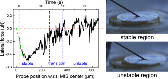
3.3. Lateral Stability

A proper characterization of the PM stability is important for any potential application of MIS, such as micro-gyroscopes or micro-motors. However, previous work only discussed simulation results with respect to lateral force and PM lateral displacement [9,22]. We herewith experimentally investigate the lateral stability by means of measuring lateral force Fr in the lateral displacement of the PM with a mechanical probe (FT-FS1000, FEMTO-TOOLS AG, Buchs, Switzerland) and a microforce sensing probe (FT-S100, FEMTO-TOOLS AG) with a force and linear displacement resolution of 5 nN and 5 nm, respectively. The mechanical probe was placed under a 30° with respect to the plane of the PM and inserted into a hole with a diameter of 400 μm cut in the middle of the PM, as depicted in Figure 9b. The probe is able to move at a constant step speed and record the force together with the displacement. The force vs. displacement curve is presented in Figure 9a, and a movie of the experiment has been included as Supplementary Material. Due to the fact that the PM was displaced in a controlled manner, a straightforward correlation of the graphic in Figure 9a and the movie is possible, and therefore, the time axis has been included in Figure 9a.
The analysis of Figure 9a shows that the behavior of the lateral force can be defined in three regions of lateral displacement, namely stable, transition and unstable. In the stable region from 0 to 260 μm, the lateral force is a restoring force, pushing the PM back to the equilibrium position. In the transition region defined by the two blue dashed lines, Fr approaches zero. In the unstable region, Fr is a runaway force, pushing the PM away from the equilibrium position.
The lateral stability can also be investigated from an energetic point of view. The lateral force and system energy can be linked according to the definition:
F r = W r
where W and r are the system energy and the displacement in the radial direction, respectively. The profile of the system energy has been obtained by 2D COMSOL simulation (Figure 9c). The exact transition point between the stable and unstable region is where the energy reaches the maximum and its derivative Fr becomes zero. The difference between simulation and experiment should have been due to the 2D model, lacking of PM velocity and collisions. It is worth noting that the PM is less stable (the potential energy well is shallower) and less confined (the stability region is wider) for higher levitation heights.

3.4. Temperature

Another major issue in using the electromagnetic induction in micro-devices is the large current density required due to scaling down, thus leading to increasing heat dissipation and temperatures in micro-devices, which may cause melting, metal delamination, oxidation and, eventually, complete device failure. For the 2D MIS in [8], the temperature of the coil was reported to be 600 °C. Because the 3D MIS offers the possibility to employ lower currents, it also seems more competitive from the point of view of the heat dissipated in the device volume. On the other hand, the higher density of windings of the 3D MIS means that the heat is generated in a relatively small volume, and it may be difficult to efficiently evacuate the heat in order to prevent device over heating.
We measured the temperature distribution when the PM was levitated at 120 μm as shown in Figure 10. The maximum temperature was 112 °C at the outer coil. Then, by removing the PM, but maintaining the corresponding excitation of the two coils, we measured the maximum temperature of 131 °C at the inner coil, significantly lower than the 2D MIS reported in [8]. The PM temperature was measured to be around 50 °C, similar to what has been reported in [8]. It is noticed that the edge temperature is larger than the center part of the PM. This is due to convection from the heating source of the inner coil and the eddy current distribution, as shown in [12].

4. Conclusions

The present paper provides a comprehensive characterization of the MIS performance in terms of levitation height as a function of the input parameters, i.e., the amplitude and frequency of the excitation currents, as well as the theoretical model to estimate the current versus frequency dependence for a given constant height of the proof mass. We have shown in this paper that there are clear advantages in employing 3D wire-bonded microcoils in the development of micromachined inductive suspensions, over the use of 2D planar microcoils. The main advantage is related to the possibility of having a tremendously higher number of coil windings, therefore increasing the ampere-turn value. This increased number of windings is achieved in one single process step, as opposed to the planar coils, where each additional winding introduces several process steps. As a consequence, the current amplitudes needed to achieve similar levitation performance are reduced dramatically compared to the 2D case. However, we have also emphasized the precautions that must be taken in the case of using 3D coil structures. These are related mainly to the range of operating frequencies, which is significantly reduced to a much smaller value for the self-resonant frequency of these 3D structures compared to their 2D counterparts. The 3D microcoils demonstrated here also show a significantly improved temperature behavior compared with planar microcoils.

Supplementary Materials

Supplementary materials can be accessed at: https://www.mdpi.com/2072-666X/5/4/1469/s1.

Acknowledgments

Zhiqiu Lu gratefully acknowledges the support from the Siemens-DAAD (German Academic Exchange Service) Scholarship. Kirill Poletkin acknowledges with thanks the support of the Alexander von Humboldt Foundation (Grant RUS-1149346 STP). Vlad Badilita kindly acknowledges support from the German Research Foundation (DFG) through Project Number BA 4275/2-1. We further thank Ali Moazenzadeh for wire bonding technical support, Kay Steffan for doing Au electroplating, the Laboratory for Electrical Instrumentation at IMTEK for high frequency measurements and the electronic service center at IMTEK for the PCB design and discussions.

Author Contributions

Zhiqiu Lu, Kirill Poletkin, Ulrike Wallrabe and Vlad Badilita planned the experiments. Zhiqiu Lu performed most of the experiments and the fabrication. Zhiqiu Lu and Kirill Poletkin prepared the figures. Kirill Poletkin prepared the theory section. Zhiqiu Lu, Kirill Poletkin and Vlad Badilita wrote the manuscript. All authors reviewed the manuscript.

Conflicts of Interest

The authors declare no conflict of interest.

References

  1. Souza, G.R.; Molina, J.R.; Raphael, R.M.; Ozawa, M.G.; Stark, D.J.; Levin, C.S.; Bronk, L.F.; Ananta, J.S.; Mandelin, J.; Georgescu, M.M. Three-dimensional tissue culture based on magnetic cell levitation. Nat. Nanotechnol 2010, 5, 291–296. [Google Scholar]
  2. Khamesee, M.B.; Kato, N.; Nomura, Y.; Nakamura, T. Design and control of a microrobotic system using magnetic levitation. IEEE/ASME Trans. Mechatron 2002, 7, 1–14. [Google Scholar]
  3. Zhang, W.; Chen, W.; Zhao, X.; Wu, X.; Liu, W.; Huang, X.; Shao, S. The study of an electromagnetic levitating micromotor for application in a rotating gyroscope. Sens. Actuators A 2006, 132, 651–657. [Google Scholar]
  4. Walther, A.; Givord, D.; Dempsey, N.; Khlopkov, K.; Gutfleisch, O. Structural, magnetic, and mechanical properties of 5 μ m thick SmCo films suitable for use in microelectromechanical systems. J. Appl. Phys 2008, 103. [Google Scholar] [CrossRef] [Green Version]
  5. Moazenzadeh, A.; Spengler, N.; Wallrabe, U. High-performance, 3D-microtransformers on multilayered magnetic cores, Proceedings of 2013 IEEE 26th International Conference on Micro Electro Mechanical Systems (MEMS), Taipei, Taiwan, 20–24 January 2013; pp. 287–290.
  6. Oniku, O.D.; Bowers, B.J.; Shetye, S.B.; Wang, N.; Arnold, D.P. Permanent magnet microstructures using dry-pressed magnetic powders. J. Micromech. Microeng 2013, 23, 075027. [Google Scholar]
  7. Shearwood, C.; Williams, C.; Mellor, P.; Yates, R.; Gibbs, M.; Mattingley, A. Levitation of a micromachined rotor for application in a rotating gyroscope. Electron. Lett 1995, 31, 1845–1846. [Google Scholar]
  8. Shearwood, C.; Ho, K.; Williams, C.; Gong, H. Development of a levitated micromotor for application as a gyroscope. Sens. Actuators A Phys 2000, 83, 85–92. [Google Scholar]
  9. Wu, X.; Chen, W.; Zhao, X.; Zhang, W. Development of a micromachined rotating gyroscope with electromagnetically levitated rotor. J. Micromech. Microeng 2006, 16, 1993. [Google Scholar]
  10. Sari, I.; Kraft, M. A MEMS Linear Accelerator for Levitated Micro-objects. Sens. Actuators A Phys 2014. [Google Scholar] [CrossRef]
  11. Badilita, V.; Rzesnik, S.; Kratt, K.; Wallrabe, U. Characterization of the 2nd generation magnetic microbearing with integrated stabilization for frictionless devices, Proceedings of 2011 16th International Solid-State Sensors, Actuators and Microsystems Conference (TRANSDUCERS), Beijing, China, 5–9 June 2011; pp. 1456–1459.
  12. Lu, Z.; Jia, F.; Korvink, J.; Wallrabe, U.; Badilita, V. Design optimization of an electromangetic microlevitation system based on copper wirebonded coils, Proceddings of PowerMEMS 2012, Atlanta, GA, USA, 2–5 December 2012; pp. 363–366.
  13. Lu, Z.; Poletkin, K.; den Hartogh, B.; Wallrabe, U.; Badilita, V. 3D micro-machined inductive contactless suspension: Testing and modeling. Sens. Actuators A Phys 2014, 220, 134–143. [Google Scholar]
  14. Kratt, K.; Badilita, V.; Burger, T.; Korvink, J.; Wallrabe, U. A fully MEMS-compatible process for 3D high aspect ratio micro coils obtained with an automatic wire bonder. J. Micromech. Microeng 2010, 20, 015021. [Google Scholar]
  15. Lee, T.H. The Design of CMOS Radio-Frequency Integrated Circuits; Cambridge University Press: Cambridge, UK, 2004. [Google Scholar]
  16. Fawzi, T.; Burke, P. The accurate computation of self and mutual inductances of circular coils. IEEE Trans. Power Appar. Syst 1978, PAS-97. 464–468. [Google Scholar]
  17. Yang, Z.; Wang, G.; Liu, W. Analytical calculation of the self-resonant frequency of biomedical telemetry coils, Proceedings of 28th Annual International Conference of the IEEE Engineering in Medicine and Biology Society, New York, NY, USA, 30 August 2–3 September 2006; pp. 5880–5883.
  18. Sari, I.; Kraft, M. A micro electrostatic linear accelerator based on electromagnetic levitation, Proceedings of 2011 16th International Solid-State Sensors, Actuators and Microsystems Conference (TRANSDUCERS), Beijing, China, 5–9 June 2011; pp. 1729–1732.
  19. Poletkin, K.; Chernomorsky, A.I.; Shearwood, C.; Wallrabe, U. An analytical model of micromachined electromagnetic inductive contactless suspension, Proceedings of ASME 2013 International Mechanical Engineering Congress and Exposition, San Diego, CA, USA, 15–21 November 2013.
  20. Poletkin, K.; Chernomorsky, A.; Shearwood, C.; Wallrabe, U. A qualitative analysis of designs of micromachined electromagnetic inductive contactless suspension. Int. J. Mech. Sci 2014, 82, 110–121. [Google Scholar]
  21. Krakowski, M. Eddy-current losses in thin circular and rectangular plates. Electr. Eng 1982, 64, 307–311. [Google Scholar]
  22. Williams, C.; Shearwood, C.; Mellor, P.; Yates, R. Modelling and testing of a frictionless levitated micromotor. Sens. Actuators A Phys 1997, 61, 469–473. [Google Scholar]
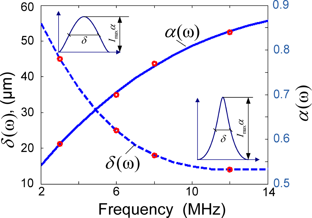
Figure 1. (a) Schematic of a 3D micromachined inductive suspension (MIS); (b) closeup of a 3D MIS without the proof mass (PM).
Micromachines 05 01469f1
Figure 2. (a) Inductance and (b) impedance measurement of coils with one layer and two layers of windings. The number of windings in the double-layer coils is twice as in the single-layer coils.
Micromachines 05 01469f2
Figure 3. (a) Schematic of the experiment setup and (b) photo of a 3D MIS on a printed circuit board.
Micromachines 05 01469f3
Figure 4. Levitation height as a function of input current frequency.
Micromachines 05 01469f4
Figure 5. (a) Levitation height as a function of RMS values of input currents. (b) Photo of a tilted PM. (c) Lorentz force distribution (red arrow) under the condition of Iouter = 2Iinner = 220 mA.
Micromachines 05 01469f5
Figure 6. The red square points are experimental measurement. The black line is the theoretical curve generated by Equation (6) assuming that δ = 20 μm and α = 0.8.
Micromachines 05 01469f6
Figure 7. Curves of α(ω) (blue line) and δ(ω) (dashed line), together with αn and δn (n = 1..4) (red circles) taken from Table 1.
Micromachines 05 01469f7
Figure 8. Current vs. frequency dependence for constant levitation height.
Micromachines 05 01469f8
Figure 9. (a) Measurement of force vs. displacement. The region between the vertical blue lines represents the transition between the two states depicted in (b); (b) captures of the lateral displacement measurement corresponding to a stable (top) and unstable (bottom) position, respectively; (c) The system energy wells obtained by 2D simulation with variable PM center position.
Micromachines 05 01469f9
Figure 10. Temperature distribution of the 3D MIS and a 3200 μm-diameter Al PM (blue in the center) after the MIS reached thermal equilibrium. The inner coil is blocked by the PM. IR camera resolution: 0.1 mm.
Micromachines 05 01469f10
Table 1. Defined α and δ for four frequency reference points.
Frequency, MHz36812
α0.590.70.770.84
δ, μm45251814

