Insect-Inspired Micropump: Flow in a Tube with Local Contractions

Abstract

A biologically-inspired micropumping model in a three-dimensional tube subjected to localized wall constrictions is given in this article. The present study extends our previous pumping model where a 3D channel with a square cross-section is considered. The proposed pumping approach herein applies to tubular geometries and is given to mimic an insect respiration mode, where the tracheal tube rhythmic wall contractions are used/hypothesized to enhance the internal flow transport within the entire respiration network. The method of regularized Stokeslets-mesh-free computations is used to reconstruct the flow motions induced by the wall movements and to calculate the time-averaged net flow rate. The time-averaged net flow rates from both the tube and channel models are compared. Results have shown that an inelastic tube with at least two contractions forced to move with a specific time lag protocol can work as a micropump. The system is simple and expected to be useful in many biomedical applications.

1. Introduction

Bioinspired micromachines are considered to be one of the most novel directions toward miniaturizing equipment for several biomedical applications. This will be made possible by developing state-of-the-art microfabrication technologies that can help in building micro- and nano-scale structures. These microstructures can be then used as components in functional micromachines, such as pumps, valves and separators, where all of these components can be built and assembled on a single chip. Here, we focus our attention on a novel micropumping paradigm that is inspired by insect respiration physiology [1,2,3,4,5,6,7,8,9].

The flow transport within insect physiological systems is complex and non-stationary because of insects’ use of body movements and rhythmic wall contractions along their tracheal tubes to enhance internal flow motions. According to the author’s knowledge, to date, there is no detailed numerical simulation study given toward understanding or resolving insect internal flow motions. However, other multiple theoretical and numerical research efforts from the literature can actually be useful when modeling these bio-fluid problems. For example, a simplified solution that can describe the unsteady viscous flow motions in a semi-infinite pipe with wall contractions or expansion modes is given in [10]. Another solution to the incompressible-viscous flow in an infinitely-long channel with prescribed pulsatile and sinusoidal wall motions is derived in [11]. Furthermore, the unsteady squeezing of a viscous fluid from a shrinking or expanding tube is given analytically in [12,13,14]. The flow in a tube due to wall contractions is also given by multiple studies [15,16,17].

The internal flow motions inside many physiological systems are normally driven by wave propagation of the muscular wall contractions, known as peristaltic pumping. Peristalsis-induced flow motions have been a main research area in classical biological fluid dynamics. There are several theoretical and numerical methods that have been used to study peristalsis-induced flow transport in two-dimensional and three-dimensional tubes [18].

In many of physiological systems that use wall contractions to transport blood or air, the kinematics of these wall motions have been shown to greatly impact the overall flow transport efficiency. Generally, there are two main types of localized wall contractions, namely stationary and progressive (local peristalsis) contractions can naturally exist in these systems, as reviewed in [19]. For example, both types have been observed in the human duodenum. These contractions have been shown to produce and enhance fluid transport in the human intestine, as well. An important conclusion from this review [19] and supported by a basic theoretical analysis is that at least two stationary contractions operating with a slight time lag (phase lag) are needed in order to produce net flow transport [20]. Additionally, insects’ tracheal tubes are another example of physiological systems that use localized wall contractions as a natural pump to deliver oxygen to the entire proximal body cells [4,5,6,7].

In this study, we extend our bioinspired micropumping models [1,2,3,4,5,6,7,8] to simulate the flow transport in a tubular geometry. In particular, we present a three-dimensional numerical simulation based on the regularized Stokeslets method of fundamental solutions (MFS) to study flow motions within an insect tracheal-like tube. Results from this study are given to complement and to strengthen our previous pumping finding, which is inspired by the rhythmic contractions found in insect tracheal tubes.

2. Methods

In this section, we use the three-dimensional Stokeslets-mesh-free computational model based on the method of regularized Stokeslets [21] to study the contraction-induced flow pumping of viscous fluid in a tube with rhythmic contractions. Results from this analysis will be compared and validated against our 2D theoretical analysis derived previously [6]. The flow structures and development in a tube with two wall contractions governed by a generic wall profile $R(z,t)$ will be given in detail. The proposed wall profile permits contractions to move with various phases (time) lags with respect to each other. The details of the computational approach used herein can be found in [18,21,22,23] and are summarized below.

The method of regularized Stokeslet [21] is based on finding exact solutions of the Stokes equations using body forces represented by smooth and localized elements, which satisfy the Stokes incompressible flow equations:

$${\nabla }^{*}·{\text{V}}^{*}=0$$

(1)

$$\mu {△}^{*}{\text{V}}^{*}={\nabla }^{*}{p}^{*}-{\text{F}}^{*}$$

(2)

where μ is the fluid viscosity, $p^{*}$ is the pressure, ${\text{V}}^{*}$ is the velocity and ${\text{F}}^{*}$ is the force per unit volume, which can be written in terms of Green’s function and regularization (cut-off) expression as,

$${\text{F}}^{*}=-{\alpha }^{*}{\varphi }^{*}\left({\text{x}}^{*}-{\text{x}}_0^{*}\right)$$

(3)

where ${\varphi }^{*}\left({\text{x}}^{*}-{\text{x}}_0^{*}\right)$ is a cut-off function with a property that $\int {\varphi }^{*}\left({\text{x}}^{*}\right)d\text{x}=1$. In our computations, we use a specific cut-off function that is given as [18],

$${\varphi }^{*}\left({\text{x}}^{*}-{\text{x}}_0^{*}\right)=\frac{15{{ϵ}^{*}}^4}{8\pi {\left({r^{*}}^2+{{ϵ}^{*}}^2\right)}^{7/2}}$$

(4)

where $r^{*}=\parallel {\text{x}}^{*}-{\text{x}}_0^{*}\parallel$. ${ϵ}^{*}$ is a small regularization parameter that is given to control the spread of the cut-off function. The velocity field and pressure solutions to the above governing equations can be given as:

$$V_i^{*}\left({\text{x}}^{*}\right)=\frac{1}{8\pi \mu }{S}_{ij}\left({\text{x}}^{*}-{\text{x}}_0^{*}\right){\alpha }_j^{*}$$

(5)

$$p^{*}\left({\text{x}}^{*}\right)=\frac{1}{8\pi }{P}_j\left({\text{x}}^{*}-{\text{x}}_0^{*}\right){\alpha }_j^{*}$$

(6)

The indices i, j = 1, 2, 3 follow the Einstein summation convention. Furthermore, $V_i^{*}=(w^{*},v^{*},u^{*})$ is the flow velocity vector, and $p^{*}$ is the static pressure. ${\text{x}}_i^{*}=(z^{*},y^{*},x^{*})$ is the position vector. ${\alpha }^{*}=({\alpha }_z^{*},{\alpha }_y^{*},{\alpha }_x^{*})$ is the force vector strength along $z^{*},y^{*},x^{*}$ directions. $S_{ij}$ is known as a regularized Stokeslet, and $P_j$ is the stress tensor, which can be given as:

$$S_{ij}={\delta }_{ij}{A}_1^{*}+\frac{\left({\text{x}}_i^{*}-{\text{x}}_0^{*}i\right)\left({\text{x}}_j^{*}-{\text{x}}_0^{*}j\right)}{A_2^{*}}$$

(7)

$$P_j=\left({\text{x}}_j^{*}-{\text{x}}_0^{*}j\right)A_3^{*}$$

(8)

where $A_1^{*}=\frac{\left({r^{*}}^2+2{ϵ}^2\right)}{{\left({r^{*}}^2+{ϵ}^2\right)}^{3/2}}$, $A_2^{*}={\left({r^{*}}^2+{ϵ}^2\right)}^{3/2}$ and $A_3^{*}=\frac{\left({2r^{*}}^2+5{ϵ}^2\right)}{{\left({r^{*}}^2+{ϵ}^2\right)}^{5/2}}$. For clarity, the velocity expression using the above equations can be easily rewritten in component form as follows,

$$\begin{array}{ccc}\hfill u^{*}& =& \frac{{\alpha }_x^{*}}{8\pi \mu A_2^{*}}\left(\frac{A_1^{*}}{A_2^{*}}+{\left(x^{*}-x_0^{*}\right)}^2\right)+\frac{{\alpha }_y^{*}}{8\pi \mu A_2^{*}}\left(x^{*}-x_0^{*}\right)\left(y^{*}-y_0^{*}\right)\hfill \\ & & +\frac{{\alpha }_z^{*}}{8\pi \mu A_2^{*}}\left(x^{*}-x_0^{*}\right)\left(z^{*}-z_0^{*}\right)\hfill \end{array}$$

(9)

$$\begin{array}{ccc}\hfill v^{*}& =& \frac{{\alpha }_x^{*}}{8\pi \mu A_2^{*}}\left(x^{*}-x_0^{*}\right)\left(y^{*}-y_0^{*}\right)+\frac{{\alpha }_y^{*}}{8\pi \mu A_2^{*}}\left(\frac{A_1^{*}}{A_2^{*}}+{\left(y^{*}-y_0^{*}\right)}^2\right)\hfill \\ & & +\frac{{\alpha }_z^{*}}{8\pi \mu A_2^{*}}\left(y^{*}-y_0^{*}\right)\left(z^{*}-z_0^{*}\right)\hfill \end{array}$$

(10)

$$\begin{array}{ccc}\hfill w^{*}& =& \frac{{\alpha }_x^{*}}{8\pi \mu A_2^{*}}\left(x^{*}-x_0^{*}\right)\left(z^{*}-z_0^{*}\right)+\frac{{\alpha }_y^{*}}{8\pi \mu A_2^{*}}\left(y^{*}-y_0^{*}\right)\left(z^{*}-z_0^{*}\right)\hfill \\ & & +\frac{{\alpha }_z^{*}}{8\pi \mu A_2^{*}}\left(\frac{A_1^{*}}{A_2^{*}}+{\left(z^{*}-z_0^{*}\right)}^2\right)\hfill \end{array}$$

(11)

Similarly, the pressure is given as:

$$p^{*}=\frac{A_3^{*}}{8\pi }\left[{\alpha }_x^{*}\left(x^{*}-x_0^{*}\right)+{\alpha }_y^{*}\left(y^{*}-y_0^{*}\right)+{\alpha }_z^{*}\left(z^{*}-z_0^{*}\right)\right]$$

(12)

Now, we consider the same non-dimensional parameters defined in [6]: let $z=z^{*}/L$, $y=y^{*}/R$, $x=x^{*}/R$, $r=r^{*}/L$, $\delta =R/L$, where R is the tube nominal radius. Furthermore, we let $w=w_x^{*}/u_o$, $v=v_r^{*}/\delta u_o$, $u=u_x^{*}/\delta u_o$, $p=p^{*}{R}^2/\left(\mu u_{o}L\right)$, ${\alpha }_z={\alpha }_z^{*}/\left(\mu u_o\right)$, ${\alpha }_y={\alpha }_y^{*}/\left(\mu u_o\right)$, ${\alpha }_x={\alpha }_x^{*}/\left(\mu u_o\right)$, $A_1=A_1^{*}/L$, $A_2=A_2^{*}/L$, $A_3=A_3^{*}/L$, $ϵ={ϵ}^{*}/L$. The above velocity expressions in component form can be rewritten in a non-dimensional form as,

$$u=\frac{{\alpha }_x}{8\pi \delta A_2}\left(\frac{A_1}{A_2}+{\delta }^2{\left(x-x_0\right)}^2\right)+\frac{{\alpha }_y\delta }{8\pi A_2}\left(x-x_0\right)\left(y-y_0\right)+\frac{{\alpha }_z}{8\pi A_2}\left(x-x_0\right)\left(z-z_0\right)$$

(13)

$$v=\frac{{\alpha }_x\delta }{8\pi A_2}\left(x-x_0\right)\left(y-y_0\right)+\frac{{\alpha }_y}{8\pi \delta A_2}\left(\frac{A_1}{A_2}+{\delta }^2{\left(y-y_0\right)}^2\right)+\frac{{\alpha }_z}{8\pi A_2}\left(y-y_0\right)\left(z-z_0\right)$$

(14)

$$w=\frac{{\alpha }_x\delta }{8\pi A_2}\left(x-x_0\right)\left(z-z_0\right)+\frac{{\alpha }_y\delta }{8\pi A_2}\left(y-y_0\right)\left(z-z_0\right)+\frac{{\alpha }_z}{8\pi A_2}\left(\frac{A_1}{A_2}+{\left(z-z_0\right)}^2\right)$$

(15)

Similarly, the non-dimensional pressure is given by:

$$p=\frac{A_3{\delta }^2}{8\pi }\left[\delta {\alpha }_x\left(x-x_0\right)+\delta {\alpha }_y\left(y-y_0\right)+{\alpha }_z\left(z-z_0\right)\right]$$

(16)

where $r=\sqrt{{\delta }^2{\left(x-x_0\right)}^2+{\delta }^2{\left(y-y_0\right)}^2+{\left(z-z_0\right)}^2}$, $A_1=\frac{\left(r^2+2{ϵ}^2\right)}{{\left(r^2+{ϵ}^2\right)}^{3/2}}$, $A_2={\left(r^2+{ϵ}^2\right)}^{3/2}$ and $A_3=\frac{\left(2r^2+5{ϵ}^2\right)}{{\left(r^2+{ϵ}^2\right)}^{5/2}}$.

3. Results and Discussion

The MFS-Stokeslets mesh-free technique is used herein to obtain the velocity field and pressure within the tube pump under consideration. The solution is formed by summing all of the Stokeslets expressions with unknown intensities. The strengths of these Stokeslets singularities can be obtained by enforcing and satisfying the prescribed boundary conditions using direct collocation approaches [24] and [21]. For the problem under consideration herein and shown in Figure 1, N Stokeslets (regularized source points) with unknown strengths α are distributed along the tube boundaries. As a result, the induced flow field by these singular points is then approximated by applying the principle of superposition and taking the effect from all Stokeslets points. The velocity field can be then evaluated as:

$$\begin{array}{ccc}\hfill u\left(x_i,y_i,z_i\right)& =& \sum _{j=1}^N\frac{{\alpha }_{xj}}{8\pi \delta A_{2j}}\left(\frac{A_{1j}}{A_{2j}}+{\delta }^2{\left(x_i-x_{0j}\right)}^2\right)+\frac{{\alpha }_{yj}\delta }{8\pi A_{2j}}\left(x_i-x_{0j}\right)\left(y_i-y_{0j}\right)\hfill \\ & & +\frac{{\alpha }_{zj}}{8\pi A_{2j}}\left(x_i-x_{0j}\right)\left(z_i-z_{0j}\right)\hfill \end{array}$$

(17)

$$\begin{array}{ccc}\hfill v\left(x_i,y_i,z_i\right)& =& \sum _{j=1}^N\frac{{\alpha }_{xj}\delta }{8\pi A_{2j}}\left(x_i-x_{0j}\right)\left(y_i-y_{0j}\right)+\frac{{\alpha }_{yj}}{8\pi \delta A_{2j}}\left(\frac{A_{1j}}{A_{2j}}+{\delta }^2{\left(y_i-y_{0j}\right)}^2\right)\hfill \\ & & +\frac{{\alpha }_{zj}}{8\pi A_{2j}}\left(y_i-y_{0j}\right)\left(z_i-z_{0j}\right)\hfill \end{array}$$

(18)

$$\begin{array}{ccc}\hfill w\left(x_i,y_i,z_i\right)& =& \sum _{j=1}^N\frac{{\alpha }_{xj}\delta }{8\pi A_{2j}}\left(x_i-x_{0j}\right)\left(z_i-z_{0j}\right)+\frac{{\alpha }_{yj}\delta }{8\pi A_{2j}}\left(y_i-y_{0j}\right)\left(z_i-z_{0j}\right)\hfill \\ & & +\frac{{\alpha }_{zj}}{8\pi A_{2j}}\left(\frac{A_{1j}}{A_{2j}}+{\left(z_i-z_{0j}\right)}^2\right)\hfill \end{array}$$

(19)

Similarly, the pressure is given by:

$$p\left(x_i,y_i,z_i\right)=\sum _{j=1}^N\frac{A_{3j}{\delta }^2}{8\pi }\left[\delta {\alpha }_{xj}\left(x_i-x_{0j}\right)+\delta {\alpha }_{yj}\left(y_i-y_{0j}\right)+{\alpha }_{zj}\left(z_i-z_{0j}\right)\right]$$

(20)

where $r_{ij}=\sqrt{{\delta }^2{\left(x_i-x_{0j}\right)}^2+{\delta }^2{\left(y_i-y_{0j}\right)}^2+{\left(z_i-z_{0j}\right)}^2}$, and ${\alpha }_{xj}$,${\alpha }_{yj}$, $A_{1j}=\frac{\left(r_{ij}^2+2{ϵ}^2\right)}{{\left(r_{ij}^2+{ϵ}^2\right)}^{3/2}}$, $A_{2j}={\left(r_{ij}^2+{ϵ}^2\right)}^{3/2}$, $A_{3j}=\frac{\left(2r_{ij}^2+5{ϵ}^2\right)}{{\left(r_{ij}^2+{ϵ}^2\right)}^{5/2}}$ and ${\alpha }_{zj}$ are the unknown force coefficients that represent the strengths of the Stokeslets in $x,y$ and z-directions, respectively. ${\text{x}}_i=(x_i,y_i,z_i)$ is the position of any field point. ${\text{x}}_{0j}=(x_{0j},y_{0j},z_{0j})$ are the locations of the Stokeslets source points. $r_{ij}=|{\text{x}}_i-{\text{x}}_{0j}|$ is the distance between any field point and another source point.

In order to determine the unknown strengths $\alpha =({\alpha }_{xj},{\alpha }_{yj},{\alpha }_{zj})$, the boundary conditions for velocity components and pressure are prescribed and collocated at the boundary field points, as shown in Figure 1a. Adding each fundamental solution using Equations (17)–(20), the final solution can be obtained by solving a system of equations:

$$\mathbb{A}\alpha =\text{b}$$

(21)

where $\mathbb{A}$ is a matrix of size $3N\times 3N$ with real entries formed by evaluating the right-hand side of the above expressions in Equations (17)–(20). b is a vector of size $1\times 3N$ of real entries formed by evaluating the left-hand sides of the same equations. In other words, all of the entries in both $\mathbb{A}$ and b are determined by enforcing the fundamental solutions to satisfy the boundary conditions by direct collocation. α represents the Stokeslets force intensities, which are to be determined by solving the above system of equations.

It should be mentioned here that, although the MFS is relatively easy to implement and does not require any meshing, it suffers from the ill-conditioning issue when finding the force strengths [21,24,25,26]. This method’s drawback can lead to inaccurate Stokeslets strength calculations and, thus, inaccuracies in finding the induced flow field. A solution to the above linear system problem can be found by either collocating the Stokeslets sources at an optimal distance away from the domain boundaries as proposed by [24] or by using regularized Stokeslets expressions as derived by [21]. Alternatively, similar results are accomplished by introducing a regularization to the matrix $\mathbb{A}$ itself [1]; this approach has been shown to provide an efficient and fast converging of the features when solving the linear system.

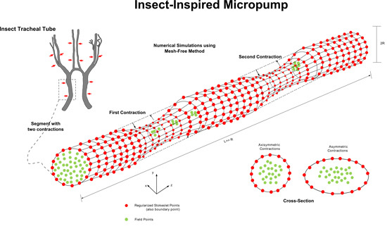
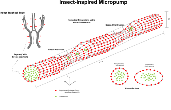
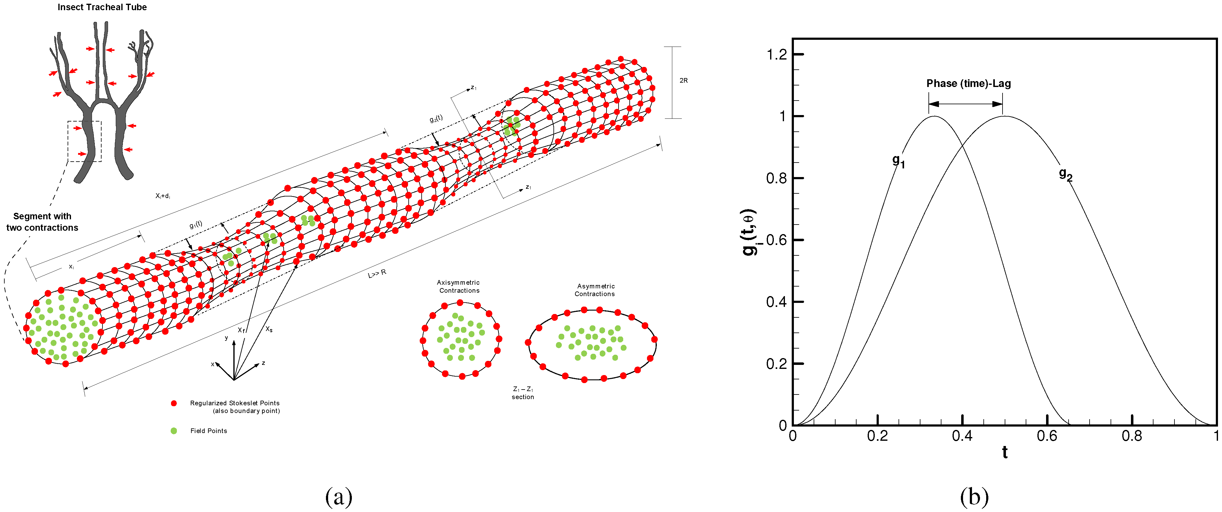
Figure 1. Problem schematic given to mimic the insect’s main tracheal tube segment with two contractions [1] and the Stokeslets-mesh-free numerical setup: (a) 3D tube with moving upper wall contraction profile $R(z,t)$; (b) $g_1\left(t\right)$ and $g_2\left(t\right)$, the motion protocols assigned to the first and second contractions, respectively.

Figure 1. Problem schematic given to mimic the insect’s main tracheal tube segment with two contractions [1] and the Stokeslets-mesh-free numerical setup: (a) 3D tube with moving upper wall contraction profile $R(z,t)$; (b) $g_1\left(t\right)$ and $g_2\left(t\right)$, the motion protocols assigned to the first and second contractions, respectively.

In this paper, we follow the algorithm given in [1] to solve for the Stokeslets strengths and to reconstruct the flow field in a 3D tube subjected to localized wall contractions that move according to a specific wall profile, as shown in Figure 1b. More details about implementing the Stokeslets-mesh-free method can be found in [2]. This section is organized as follows: Firstly, the wall profile is prescribed in full. The algorithm that will be used to overcome the ill-conditioning linear algebra issue during the calculation of the Stokeslets strengths will be given next. Thirdly, the structure and the development of the flow field induced by only two walls’ contractions that move with a non-zero phase lag will be given. Finally, the net flow rate and pumping effect will be given. The presented results are compared to our 2D theoretical solution for validation purposes [6]. The details of the subsections are given below.

3.1. Wall Profile, R(z,t)

The tube wall profile $R(z,t)$ and its contracting kinematics are prescribed using the following mathematical expressions,

$$R(z,t)=1+\sum _{i=1}^{N_c}{A}_i{f}_i\left(z\right)g_i\left(t\right)$$

(22)

where $f_i\left(z\right)\in C^r\left[0,1\right]$ and $g_i\left(t\right)\in C^r\left[0,T=1/S_t\right]$ represent the spatial and the temporal distributions of the tube surface wall shape, respectively. $N_c$ defines the number of contractions, and $A_i$ is the amplitude assigned to each contraction. The spatial term of the above equation imitates the geometry of the wall contractions as:

$$f_i\left(z\right)=tanh\left(\alpha (z-z_i)\right)-tanh\left(\alpha (z-(z_i+d_i))\right)$$

(23)

where $\alpha =2\pi /\delta$, $z_i$ defines the beginning of each collapse region and $d_i\in \left(0,1-z_i\right]$ marks its end, as shown in Figure 1b. In this work, we only consider two contractions, i.e., $N_c=2$, where the first contraction moves in time according to the following: profile:

$$g_1\left(t\right)=\left\{\begin{array}{cc}\frac{1}{2}\left(1-cos\left(2\pi \beta S_{t}t\right)\right),\hfill & 0\le t\le 1/\beta S_t\hfill \\ 0\hfill & 1/\beta S_t<t\le 1/S_t\hfill \end{array}\right.$$

(24)

while the second contraction moves according to:

$$g_2\left(t\right)=\frac{1}{2}\left(1-cos\left(2\pi S_{t}t\right)\right),0\le t\le 1/S_t$$

(25)

where the non-dimensional parameter β relates the phase lag between the first and second contractions. Although, during the compression regime, both contracting sites start to move at the same time, the first contraction reaches the maximum specified tube travel collapse (TC) distance faster than the second contraction. In other words, there will be a time lag, $T_g=(1-1/\beta )/\left(2S_t\right)$, between these two collapsing motions, which is equivalent to a phase lag ${\theta }_{12}=\pi (1-1/\beta )$. Moreover, during the expansion phase, the first contraction returns back to the nominal (original) position and continues its period with zero amplitude until the second contraction completes its own cycle; then, both contractions start the second cycle together with the protocol shown in Figure 1b. It should be noted that both contractions have a similar time period $T=1/S_t$, i.e., $S_t=1$ and that is, if $\beta =1$, there will be no phase lag and both contractions will be identical. Here, we used $z_1=0.25$, $z_2=0.65$, $d_1=d_2=0.1$, $A_1=A_2=-0.3528$, which render the maximum tube collapse ratio to be $TC=70\%$. This motion protocol has chosen, such that, after one cycle, the tube geometry will be returning to the initial position, and there will be no net flow due to any volume deformation/displacements. This proposed tube wall profile plays an important role in breaking the flow symmetry and producing a unidirectional net flow.

3.2. Algorithm for Finding Accurate Stokeslets Strengths

Finding an accurate solution to the ill-conditioned system given by Equation (21) is an important step and requires a careful implementation. The regularized parameter $ϵ=0.15$ and the total number of source points of $N=128\times 64\times 64$ have been optimized to resolve the flow details. In other words, a total number of Stokeslets $N=2^{19}$ is obtained by finding the (N-independent) solution that indeed satisfies the wall boundary conditions. This numerical algorithm follows the Tikhonov-regularization technique given in [27] to solve an ill-conditioned linear system of equations. The algorithm is based on introducing a regularization parameter, $h=0.01$, into the original matrix, $\mathbb{A}$, which is then transformed into a modified symmetric matrix, ${\mathbb{A}}_{\mathbb{R}}$. This modified matrix acts as a pre-conditioner that leads to a modified system of equations with an enhanced condition number. The algorithm is simple and only requires a priori calculations of coefficients $\mathbb{A}$, vector b, regularization parameter $h=0.01$ and a convergence criteria based on an assigned specific tolerance value $tol={10}^{-6}$. The steps of this algorithm are listed in Algorithm 1.

Algorithm 1 Algorithm for finding the strengths of each Stokeslet-source point.

Input: $\mathbb{A},\mathbb{I}\in M_{3NX3N}\left(R\right)$, b$\in R^{3N}$, h, $tol\in R$

1. ${\alpha }^{\left(\mathbf{0}\right)}$ = 0, ${\mathbf{r}}^{\left(\mathbf{0}\right)}$ =b - ${\mathbf{f}}^{\left(\mathbf{0}\right)}$ =b

2. Do while $\parallel \mathbf{r}{\parallel }_{\infty }\ge \mathbf{tol}$

3. ${\mathbb{A}}_R={\mathbb{A}}^{*}\mathbb{A}+h^2\mathbb{I}$

4. ${\alpha }^{\left(\mathbf{k}\right)}$= ${\alpha }^{(\mathbf{k}-\mathbf{1})}$+${{\mathbb{A}}_R}^{-1}{\mathbb{A}}^{*}{\mathbf{r}}^{(\mathbf{k}-\mathbf{1})}$

5. ${\mathbf{r}}^{\left(\mathbf{k}\right)}=\text{b}-\mathbb{A}{\alpha }^{\left(\mathbf{k}\right)}$

end Do

Output: Stokeslets strengths: $\alpha ={\left[{\alpha }_{xj}{\alpha }_{yj}{\alpha }_{zj}\right]}^T$, $j=1:3N$

As a direct implementation of the above algorithm, results for both velocity field and pressure induced by tube wall motions are given and compared to our 2D analytical solution [6]. More specifically, a tube with two walls collapses that move with a phase lag of ${\theta }_{12}=30$° is considered. Flow field snapshots at compression time $t=t/4$ and expansion time $t=3T/4$ are explained and used to carry out these comparisons.

3.3. Tube with Two Local Rhythmic Wall Contractions

The method of fundamental solution MFS along with the regularized Stokeslets approach are used to solve for the induced flow field in a three-dimensional tube with two moving wall contractions. The contractions are assigned to the tube wall profile $R(x,t)$ in a specific protocol to grantee net flow production. A schematic to the problem setting, along with the distribution pattern of the source points, is given in Figure 1a. The motion protocol used to actuate wall contractions is shown in Figure 1b. The goal of this section is to perform 3D simulations and to compare the results to our previously-derived 2D analytical model [6]. In addition, the net flow rate is also computed and compared to the 2D scenario. In other words, results from both the 3D Stokeslets mesh-free computations and from the 2D theoretical model are compared at different snapshots. The comparison process is given at two snapshots of times $t=T/4$ and $3T/4$ to represent compression and expansion collapsing phases, respectively. A phase lag ${\theta }_{12}={30}^{\circ }$ is used to set the contraction time between the collapsing sites.

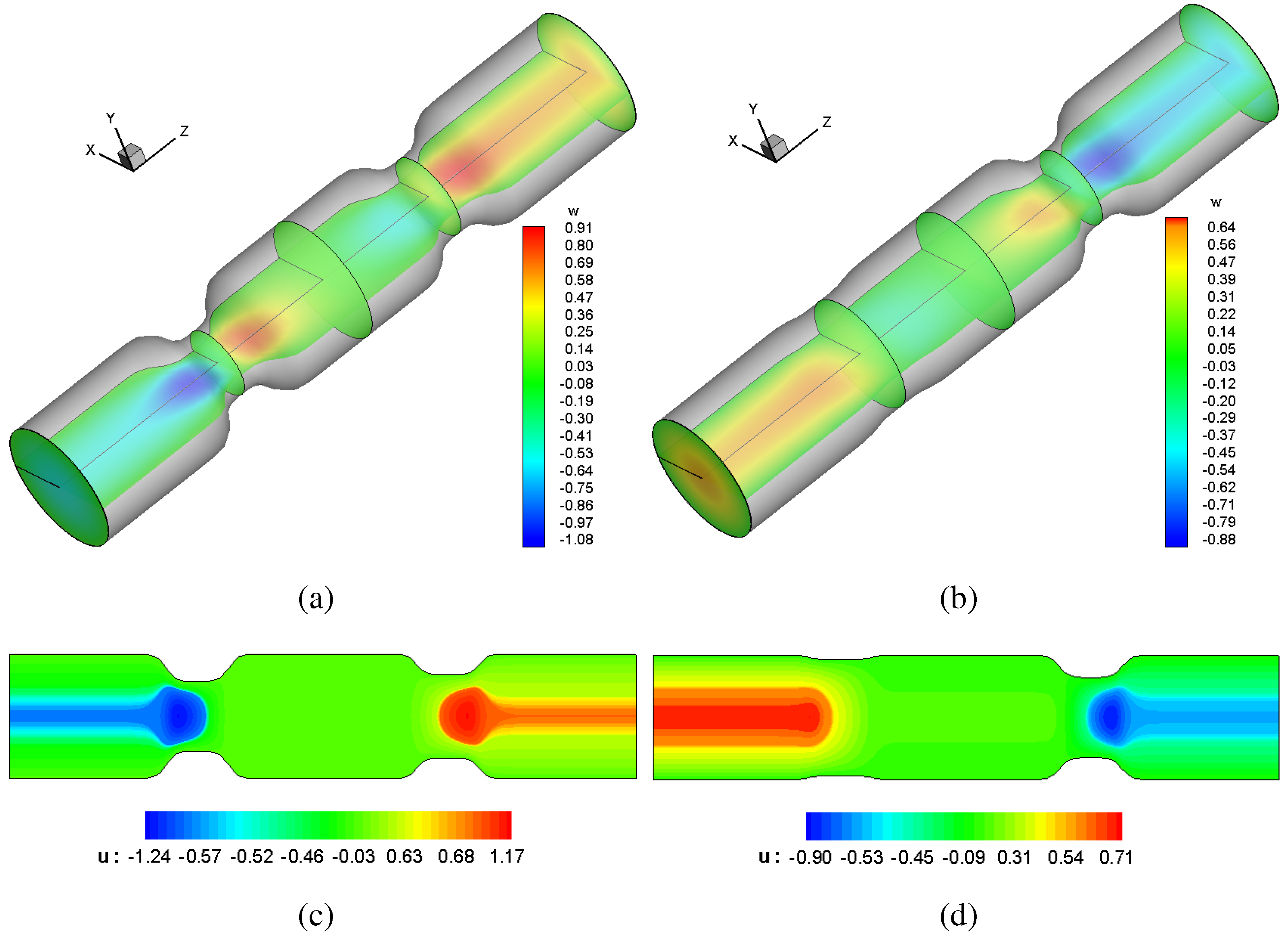
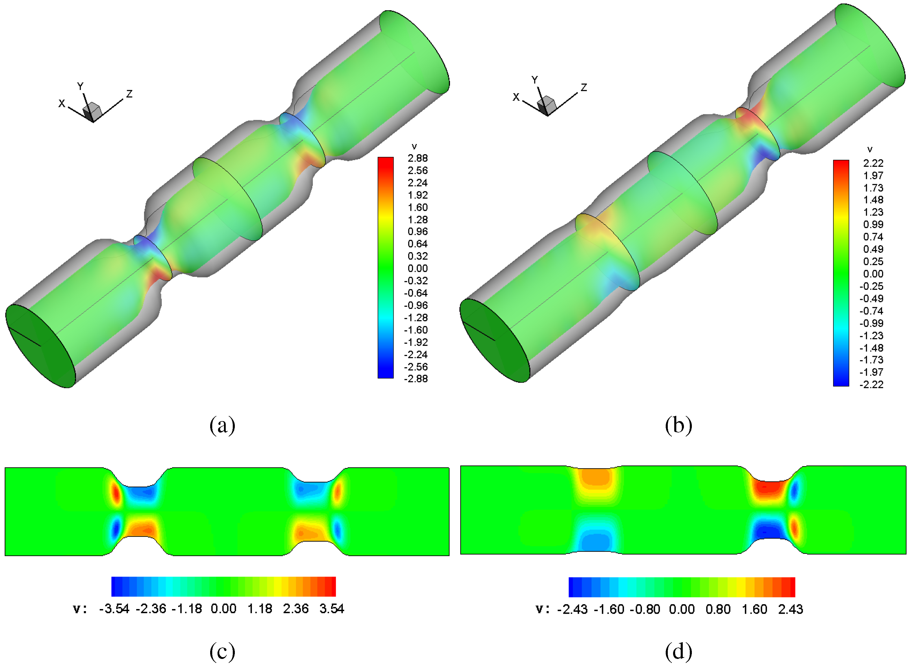
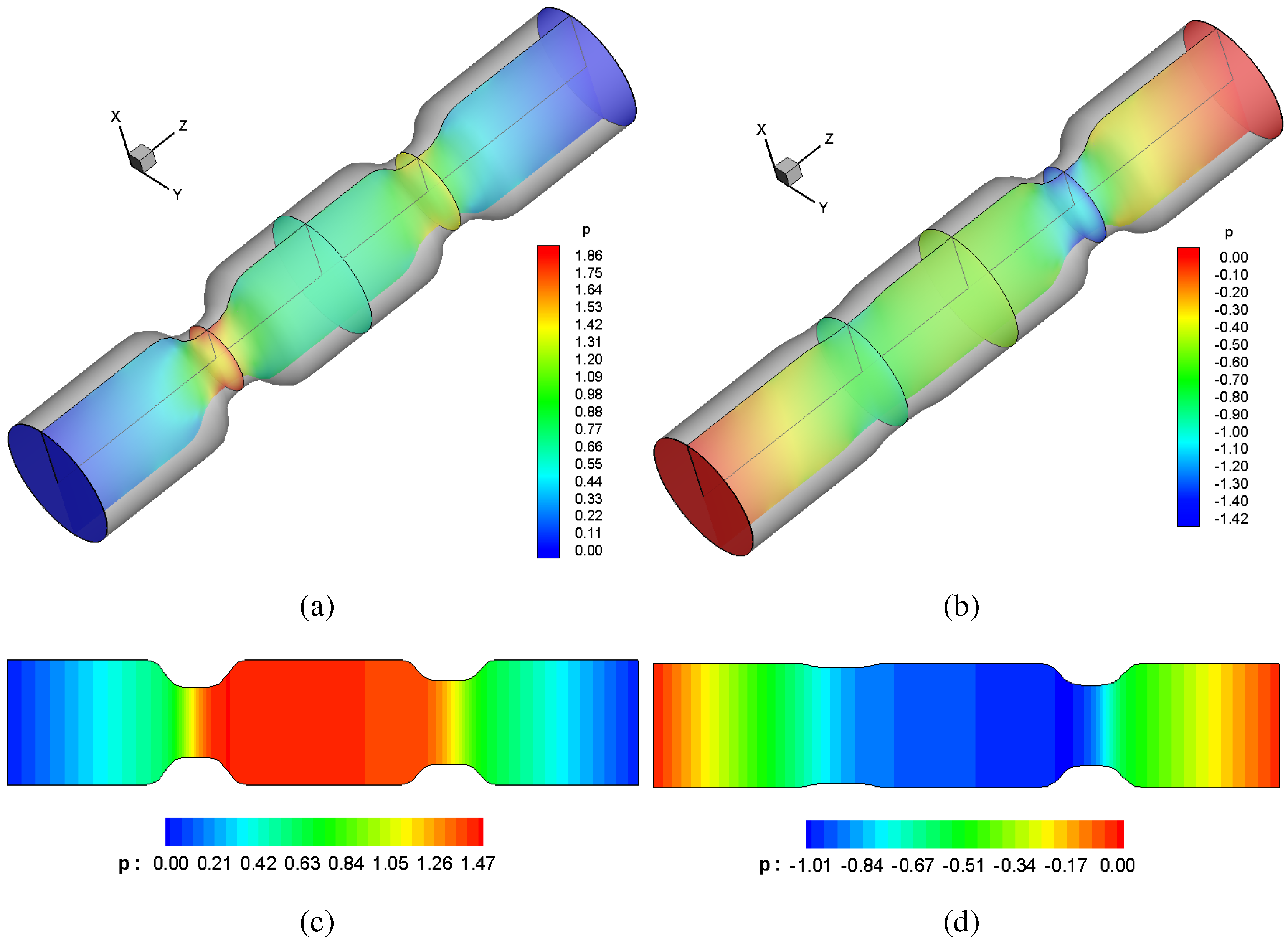
The velocity field and axial pressure are computed and shown in Figure 2, Figure 3 and Figure 4 using contour plots. Results have shown that, when ${\theta }_{12}={30}^{\circ }$, the stagnation zone between contraction sites (observed when ${\theta }_{12}=0^{\circ }$, [6]) is removed, and there exists flow transport within the region between the two contractions, as shown by the axial and vertical velocity contour lines calculated analytically and numerically, as shown in Figure 2 and Figure 3. Moreover, there are pressure gradients in the region between contraction spots, which indicate that there is a flow transport in this region, as shown in Figure 4.

Figure 2. Axial velocity contour lines: (a) 3D computations at $t=T/4$, ${\theta }_{12}={30}^{\circ }$; (b) 3D computations at $t=3T/4$, ${\theta }_{12}={30}^{\circ }$; (c) 2D theory at $t=T/4$, ${\theta }_{12}={30}^{\circ }$; (d) 2D theory at $t=3T/4$, ${\theta }_{12}={30}^{\circ }$.

Figure 2. Axial velocity contour lines: (a) 3D computations at $t=T/4$, ${\theta }_{12}={30}^{\circ }$; (b) 3D computations at $t=3T/4$, ${\theta }_{12}={30}^{\circ }$; (c) 2D theory at $t=T/4$, ${\theta }_{12}={30}^{\circ }$; (d) 2D theory at $t=3T/4$, ${\theta }_{12}={30}^{\circ }$.

Figure 3. Vertical velocity contour lines: (a) 3D computations at $t=T/4$, ${\theta }_{12}={30}^{\circ }$; (b) 3D computations at $t=3T/4$, ${\theta }_{12}={30}^{\circ }$; (c) 2D theory at $t=T/4$, ${\theta }_{12}={30}^{\circ }$; (d) 2D theory at $t=3T/4$, ${\theta }_{12}=0^{\circ }$.

Figure 3. Vertical velocity contour lines: (a) 3D computations at $t=T/4$, ${\theta }_{12}={30}^{\circ }$; (b) 3D computations at $t=3T/4$, ${\theta }_{12}={30}^{\circ }$; (c) 2D theory at $t=T/4$, ${\theta }_{12}={30}^{\circ }$; (d) 2D theory at $t=3T/4$, ${\theta }_{12}=0^{\circ }$.

Figure 4. Pressure contour lines: (a) 3D computations at $t=T/4$, ${\theta }_{12}={30}^{\circ }$; (b) 3D computations at $t=3T/4$, ${\theta }_{12}={30}^{\circ }$; (c) 2D theory at $t=T/4$, ${\theta }_{12}={30}^{\circ }$; (d) 2D theory at $t=3T/4$, ${\theta }_{12}={30}^{\circ }$.

Figure 4. Pressure contour lines: (a) 3D computations at $t=T/4$, ${\theta }_{12}={30}^{\circ }$; (b) 3D computations at $t=3T/4$, ${\theta }_{12}={30}^{\circ }$; (c) 2D theory at $t=T/4$, ${\theta }_{12}={30}^{\circ }$; (d) 2D theory at $t=3T/4$, ${\theta }_{12}={30}^{\circ }$.

3.4. Unidirectional Net Flow

The above results suggest that when the wall contractions move with different time (phase) lags, the system can be used to create a unidirectional flow and be used as a micropump. The velocity fields at different phase lags and at each time elapse during the contraction cycle are then used to calculate the time-averaged net flow rate $Q_T$ as a function of the contraction phase lag ${\theta }_{12}$ parameter. To calculate the time averaged net flow rate, the instantaneous flow rate at a desired location along the axial direction is calculated firstly. The details of how the time averaged net flow rate is calculated can be also found in [18], which can be re-given as follows:

$$q(z,t)={\int }_{A(z,t)}Q(x,y,z,t)dydx$$

(26)

where $A(z,t)$ is the cross-sectional area along the tube length z and time t. The above integration is approximated numerically using the standard trapezoidal rule. Once we have computed the instantaneous flow rate $q(z,t)$, we can average it over one period of time $T=1/S_t$. The time-averaged net flow rate is simply computed by averaging computed values at discrete times, since the flow rate is a periodic function of time. The time-averaged net flow rate per unit length of the channel is computed by:

$$Q_T\left(z\right)=\frac{1}{T}{\int }_0^{T}q(z,t)dt$$

(27)

where $T=1/S_t$ is the time period. In the discrete form, the time-averaged net flow rate can be computed using the quadrature trapezoidal rule,

$$Q_T\left(z\right)\approx \frac{1}{T}\sum _0^{n\Delta t}q(z,n\Delta t)\Delta t$$

(28)

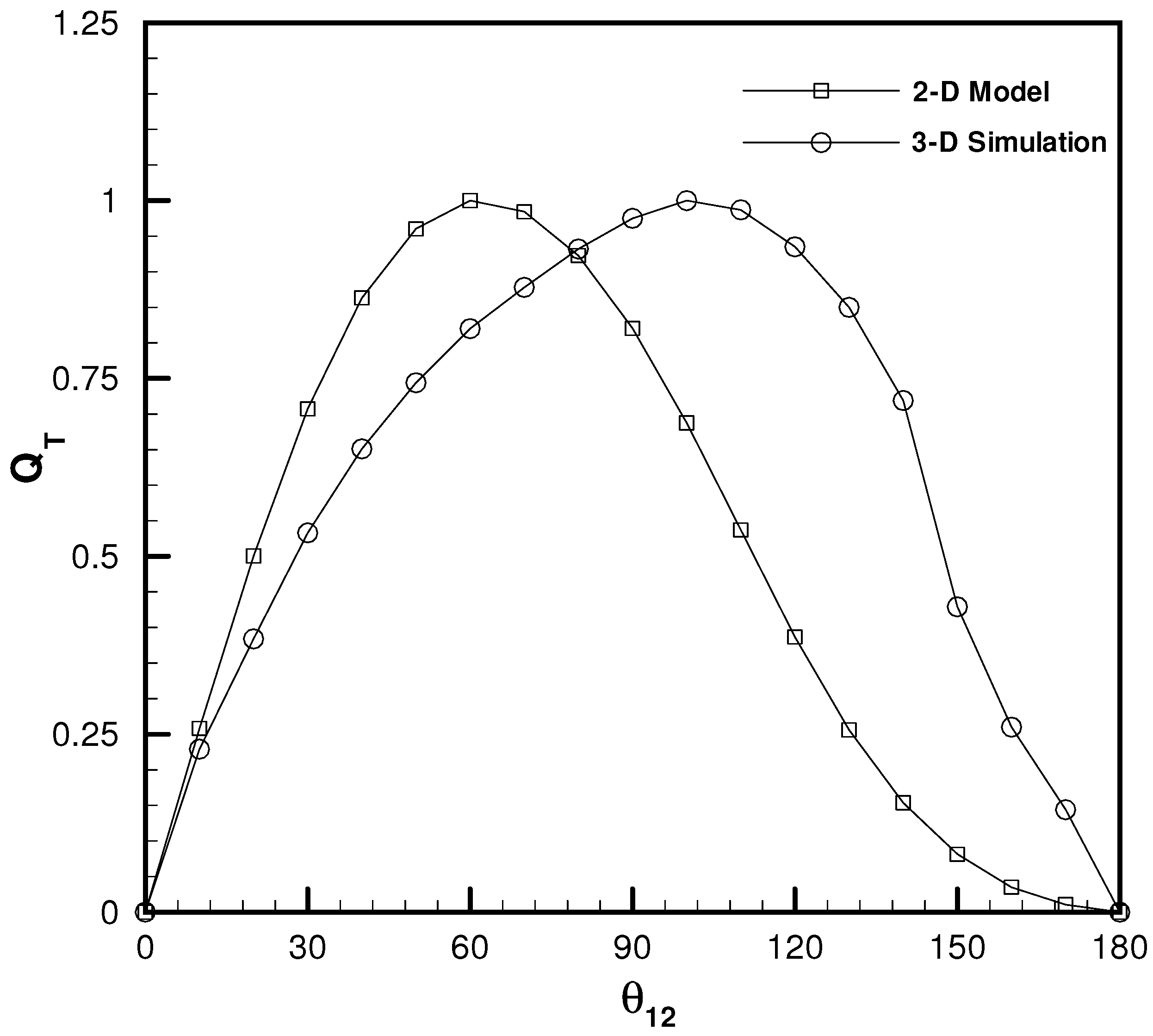
where $\Delta t=T/N_T$, $N_T$ is the number of quadrature points in a time period $T=1/S_t$. In Figure 5, we show the time-averaged net flow rate as a function of the phase lag parameter. In the same figure, results obtained by the 2D analytical solution [6] are compared to the 3D Stokeslets-mesh-free computations for the tube pumping model. Results have shown that, although there is not good agreement between 3D tube and the 2D analytical model, the net flow rate using the 3D computations has a similar trend as the 2D analytical solution. Furthermore, the maximum value of the net flow occurs at ${\theta }_{12}={110}^{\circ }$ compared to ${\theta }_{12}={65}^{\circ }$, which is predicted previously by the 2D analytical model. This phase lag discrepancy between the 2D and 3D results might be related to the three-dimensional effect, where the net flow is expected to depend on all spatial dimensions and not only on the z-direction, as assumed in the 2D counterpart. Although the net flow rate distribution as a function of phase lag of both 3D Stokeslets-mesh-free computations and 2D analytical results are different, they still share similar physical interpretations about our pumping hypotheses, which is inspired by insects’ respiration process and its rhythmic tracheal wall collapses.

Figure 5. Time-averaged net flow rate comparisons between the 2D analytical solution and 3D Stokeslets-mesh-free computations.

Figure 5. Time-averaged net flow rate comparisons between the 2D analytical solution and 3D Stokeslets-mesh-free computations.

3.5. Channel vs. Tube Simulations

The present study is a natural extension to our previously-published pumping model in a 3D channel with a square cross-section [7]. Results have shown that the flow field obtained by both the tube and channel is analogous and exhibits similar structures during the compression and the relaxation phases. This is not surprising, since both conduits have similar undeformed volume and the wall contractions are driven by the same wall profile protocol. The flow rate obtained by the tube simulation has been found to be $\sim 4$-fold greater than the channel flow rate. However, the maximum flow rate for both the tube and channel occurs at almost the same phase lag angle, i.e., at ${\theta }_{12}\simeq$ 105${}^{\circ }$–110${}^{\circ }$.

The observed increase in the tube net flow rate can simply be explained as follows: in the channel case, we only constrict from the upper walls, while in the tube case, contractions occur along the entire circumference. This means that the total deformation (volume change) over a collapsing cycle for the tube case is greater than the channel setup. We expect that when both the tube and the channel undergo similar deformations over the collapsing cycle, they will produce a similar net flow rate.

Finally, it should be noted that the tube simulation is more relevant when mimicking the physiological behavior of insect tracheal tubes. Additionally, the tube results can serve as a guide to design novel tubular micropumps for several biomedical applications. For example, a vessel-like (tubular conduit) one with multiple contractions can be designed, actuated properly and be used as a heart assist device. This might be made possible by the current revolution in nanotechnology, tissue engineering and artificial muscles.

4. Conclusions

Inspired by the insect respiration processes and their internal flow motions, a pumping model in a three-dimensional tube subjected to two rhythmic wall contractions is proposed. The flow field and time-averaged net flow rate induced by these wall contractions are reconstructed using the regularized Stokeslets-mesh-free method. Numerical results are compared to our previously-derived two-dimensional analytical pumping model. The flow field at different time snapshots has been found to be in good agreement with the 2D solution. The net flow rate over a complete cycle shows a distinct difference. In particular, the maximum net flow rate occurs at a phase lag that is different from what has been obtained using the 2D analytical model. In spite of the observed differences in the net flow rate calculations between the 3D simulations and the 2D model, the proposed system is capable of producing unidirectional flows and can be used as a micropump. This simple pump is hypothesized to be useful in building a bioinspired set of micromachines for the next generation of biomedical applications.

References

- Aboelkassem, Y.; Staples, A.E. Flow transport in a microchannel induced by moving wall contractions: A novel micropumping mechanism. Acta Mech. 2012, 223, 463–480. [Google Scholar] [CrossRef]
- Aboelkassem, Y.; Staples, A.E. Stokeslets-mesh-free computations and theory for flow in a collapsible microchannel. Theor. Comput. Fluid Dyn. 2012, 27, 681–700. [Google Scholar] [CrossRef]
- Aboelkassem, Y.; Staples, A.E.; Socha, J. Microscale flow pumping inspired by rhythmic tracheal compressions in insects. In Proceedings of the ASME Pressure Vessels and Piping Conference, Baltimore, Maryland, USA, 17–21 July 2011; Volume 4, pp. 471–479.
- Aboelkassem, Y. Novel Bioinspired Pumping Models for Microscale Flow Transport. PhD. Thesis, Virginia Tech, Blacksburg, VA, USA, 2012. [Google Scholar]
- Aboelkassem, Y.; Staples, A.E. Selective pumping in a network: Insect-style microscale flow transport. Bioinspir. Biomim. 2013, 8, 026004. [Google Scholar] [CrossRef] [PubMed]
- Aboelkassem, Y.; Staples, A.E. A bioinspired pumping model for flow in a microtube with rhythmic wall contractions. J. Fluids Struct. 2013, 42, 187–204. [Google Scholar] [CrossRef]
- Aboelkassem, Y.; Staples, A.E. A three-dimensional model for flow pumping in a microchannel inspired by insect respiration. Acta Mech. 2014, 225, 493–507. [Google Scholar] [CrossRef]
- Aboelkassem, Y. A Ghost-Valve micropumping paradigm for biomedical applications. Biomed. Eng. Lett. 2015, 5, 45–50. [Google Scholar] [CrossRef]
- Chu, A.K.H. Transport Control within a Microtube. Phys. Rev. E 2004, 70, 061902. [Google Scholar] [CrossRef]
- Uchida, S.; Aoki, H. Unsteady Flows in a Semi-infinite Contracting or Expanding Pipe. J. Fluid Mech. 1977, 82, 371–387. [Google Scholar] [CrossRef]
- Secomb, T. Flow in a channel with Pulsating Walls. J. Fluid Mech. 1978, 88, 273–288. [Google Scholar] [CrossRef]
- Skalak, F.; Wang, C.Y. On the Unsteady Squeezing of a Viscous Fluid from a Tube. J. Austral. Math. Soc. 1978, 21, 65–74. [Google Scholar] [CrossRef]
- Wang, C.Y. Arbitrary Squeezing of Fluid from a Tube at Low Squeeze Numbers. J. Appl. Math. Phys. (ZAMP) 1980, 31, 620–627. [Google Scholar] [CrossRef]
- Singh, P.; Radhakrishnan, V.; Narayan, K.A. Squeezing Flow Between Parallel Plates. Ingenieur-Archiv 1990, 60, 274–281. [Google Scholar] [CrossRef]
- Pedley, T.; Stephanoff, K.D. Flow along Channel with a Time-Dependent Indentation in One Wall: The Generation of Vorticity Waves. J. Fluid Mech. 1985, 160, 337–367. [Google Scholar] [CrossRef]
- Ralph, M.; Pedley, T.J. Flow in a Channel with Moving Indentation. J. Fluid Mech. 1988, 190, 87–112. [Google Scholar] [CrossRef]
- Mahmood, T.; Merkin, J. The flow in a narrow duct with an indentation or hump on one wall. Warme-und Stoffubertrangung 1990, 22, 69–76. [Google Scholar] [CrossRef]
- Aranda, V.; Cortez, R.; Fauci, L. Stokesian peristaltic pumping in a three-dimensional tube with a phase-shift asymmetry. Phys. Fluids 2011, 23, 081901. [Google Scholar] [CrossRef]
- Macagno, E.; Christensen, J. Fluid mechanics of the duodenum. Ann. Rev. Fluid Mech. 1980, 12, 139–158. [Google Scholar] [CrossRef]
- Macagno, E.; Christensen, J.; Lee, L. Modeling the effect of wall movement on absorption in the intestine. Am. J. Physiol. 1982, 243, G541–G550. [Google Scholar] [PubMed]
- Cortez, R. The method of regularized Stokeslets. SIAM J. Sci. Comput. 2001, 23, 1204–1225. [Google Scholar] [CrossRef]
- Cortez, R.; Fauci, L.; Medovikov, A. The method of regularized Stokeslets in three dimensions: analysis, validation, and applications to helical swimming. Phys. Fluids 2005, 17, 031504. [Google Scholar] [CrossRef]
- Ainley, J.; Durkin, S.; Embid, R.; Boindala, P.; Cortez, R. The method of images for regularized Stokeslets. J. Comput. Phys. 2008, 227, 4600–4616. [Google Scholar] [CrossRef]
- Young, D.L.; Jane, S.J.; Fan, C.M.; Murugesan, K.; Tsai, C.C. The method of fundamental solutions for 2D and 3D Stokes problems. J. Comput. Phys. 2006, 211, 1–8. [Google Scholar] [CrossRef]
- Alves, C.; Silvestre, A. Density results using Stokeslets and a method of fundamental solutions for the Stokes equations. Eng. Anal. Bound. Elem. 2004, 28, 1245–1252. [Google Scholar] [CrossRef]
- Young, D.L.; Chen, C.; Fan, C.M.; Murugesan, K.; Tsai, C.C. The method of fundamental solutions for Stokes flow in a rectangular cavity with cylinders. J. Mech. B/Fluids 2005, 24, 703–716. [Google Scholar] [CrossRef]
- Neumaier, A. Solving Ill-Conditioned and Singular Linear Systems : A Tutorial on Regularization. SIAM Rev. 1998, 40, 636–666. [Google Scholar] [CrossRef]
© 2015 by the author; licensee MDPI, Basel, Switzerland. This article is an open access article distributed under the terms and conditions of the Creative Commons Attribution license (http://creativecommons.org/licenses/by/4.0/).
Share and Cite
MDPI and ACS Style
Aboelkassem, Y. Insect-Inspired Micropump: Flow in a Tube with Local Contractions. Micromachines 2015, 6, 1143-1156. https://doi.org/10.3390/mi6081143
AMA Style
Aboelkassem Y. Insect-Inspired Micropump: Flow in a Tube with Local Contractions. Micromachines. 2015; 6(8):1143-1156. https://doi.org/10.3390/mi6081143
Chicago/Turabian StyleAboelkassem, Yasser. 2015. "Insect-Inspired Micropump: Flow in a Tube with Local Contractions" Micromachines 6, no. 8: 1143-1156. https://doi.org/10.3390/mi6081143