Micro-Machined Flow Sensors Mimicking Lateral Line Canal Neuromasts

Abstract

Fish sense water motions with their lateral line. The lateral line is a sensory system that contains up to several thousand mechanoreceptors, called neuromasts. Neuromasts occur freestanding on the skin and in subepidermal canals. We developed arrays of flow sensors based on lateral line canal neuromasts using a biomimetic approach. Each flow sensor was equipped with a PDMS (polydimethylsiloxane) lamella integrated into a canal system by means of thick- and thin-film technology. Our artificial lateral line system can estimate bulk flow velocity from the spatio-temporal propagation of flow fluctuations. Based on the modular sensor design, we were able to detect flow rates in an industrial application of tap water flow metering. Our sensory system withstood water pressures of up to six bar. We used finite element modeling to study the fluid flow inside the canal system and how this flow depends on canal dimensions. In a second set of experiments, we separated the flow sensors from the main stream by means of a flexible membrane. Nevertheless, these biomimetic neuromasts were still able to sense flow fluctuations. Fluid separation is a prerequisite for flow measurements in medical and pharmaceutical applications.

1. Introduction

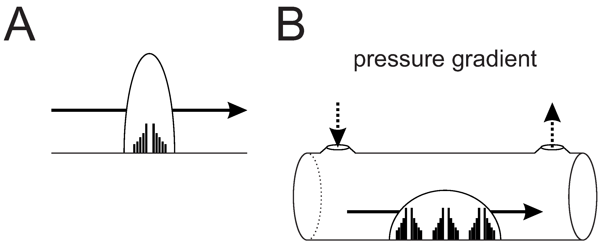
1.1. The Fish Lateral Line: A Biological Blueprint for Sensor Development

The mechanosensory lateral line of fish is sensitive to weak water motions and local pressure gradients [1,2,3,4,5,6,7]. The lateral line contains up to several thousand mechanosensors, called neuromasts [8,9]. The sensory epithelium of a neuromast consists of up to 3000 directional sensitive hair cells. The ciliary bundles of each hair cell project into a gelatinous structure, called the cupula [10,11,12,13]. Local water motions displace the cupula and, thus, deflect the ciliary bundles. This leads to an electrical response of the hair cells. Within the sensory epithelium, the hair cells of a neuromast are oriented in two opposing directions [14,15,16]. This antagonistic arrangement is the reason for the directional sensitivity of lateral line neuromasts [17,18,19].

Lateral line neuromasts occur freestanding on the skin (superficial neuromasts or SNs; Figure 1A) and in subepidermal canals (canal neuromasts or CNs; Figure 1B). CNs are embedded in fluid-filled canals connected to the ambient water via small pores [20,21]. Consequently, CNs detect fluid motions inside the canal caused by pressure gradients between adjacent canal pores [22]. Since the neuronal responses of primary lateral line afferents depend on both stimulus amplitude and stimulus direction, they cannot encode the direction of water flow unambiguously.

Figure 1. Scheme of the lateral line system. (A) Superficial neuromasts (SNs) are located on the skin of the animal and are sensitive to flow velocity; (B) canal neuromasts (CNs) are located in subepidermal canals. They are sensitive to fluid motion inside the canal caused by pressure gradients between adjacent canal pores. Solid-lined arrows indicate fluid motion; dashed-lined arrows indicate pressure acting on the pores. Modified from [23].

Figure 1. Scheme of the lateral line system. (A) Superficial neuromasts (SNs) are located on the skin of the animal and are sensitive to flow velocity; (B) canal neuromasts (CNs) are located in subepidermal canals. They are sensitive to fluid motion inside the canal caused by pressure gradients between adjacent canal pores. Solid-lined arrows indicate fluid motion; dashed-lined arrows indicate pressure acting on the pores. Modified from [23].

Many fish species live in running water. These fish can sense bulk flow velocity and bulk flow direction. Due to the filter properties of lateral line canals, the CNs of fish do not respond to the directed current component of water flow, but to the small fluctuations superimposed on the flow [24]. Fish presumably estimate the direction of flow and the flow velocity from the spatial-temporal propagation of flow fluctuations [25].

1.2. Biomimetic Flow Sensors: State of the Art

Fluid flow metering is a common task in many industrial and scientific applications. Most flow metering devices are based on vanes, hot wire anemometers, ultra sound devices, particle imaging velocimetry, Coriolis force, inductive coupling and vortex shedding [26,27,28,29,30,31]. Most of these systems are not only rather complex and have macroscopic dimensions, but in addition are expensive and/or have a high power consumption. Thus, commercially available metering systems are often limited in their applications. During the last decade, biomimetic solutions emerged in fluid dynamics. Due to the small size, striking functionality and high sensitivity of biological flow sensors, engineers started to fabricate flow sensors inspired by the fish lateral line [2,5,28,32,33,34,35]. Commonly, the biomimetic approaches intend to improve the state-of-the-art techniques used in flow sensing, e.g., underwater navigation of autonomous robots, passive sonar applications or flow metering [28,36,37].

With the exception of the hot-wire array presented by Yang et al. [28], biomimetic approaches picked up fluid motion by means of a flow-induced deflection of a cantilever-like or lamella-shaped structure (an artificial cupula), which was detected by piezo-electric [38], resistive [39,40,41,42,43], capacitive [44,45,46], ionic polymer-metal composite (IPMC)-based [29,47] or optical [48,49,50,51] read-out techniques.

The most prominent solutions of mimicking biomimetic flow sensors are based on piezo-resistive detection systems. In these systems, the bending of a cantilever is detected with a piezo-resistive stress-strain gauge. One example of a cantilever-based hair cell sensor with a piezo-resistive read-out system is given by Yang et al. [34]. Their artificial neuromasts were made of SU-8 and based on a piezo-resistive stress-strain gauge. Other authors developed piezo-resistive artificial flow sensors with a sensitivity comparable to that of the fish lateral line [39,41,43,52]. Fan et al. [53] introduced a striking technique to fabricate out-of-plane cantilevers made from metal and polymer that also acted as a stress gauge. Unfortunately, the above structures are very fragile and suffer from non-uniformity during fabrication. Qualtieri et al. [54,55] introduced a waterproof system mimicking SNs that was also based on a piezo-resistive detection principle. Their self-binding cantilevers consisted of Si, SiO₂, SiN₄ or aluminum nitride. To achieve a waterproof operation, the sensors were coated with parylene-C. Piezo-resistive read-out techniques were also used to fabricate a bioinspired inclinometer and a miniaturized hydrophone [56,57,58]. In addition, miniaturized hydrophone arrays using the resistive detection principle were built to imitate fish lateral lines [59]. Due to its design, in particular the metallization process resulting in a low bending of the a stiff membrane, this sensor only had a sensitivity of about 1 Pa.

Capacitive detection systems were used to imitate sensory hairs found on cricket cerci [44,45,60,61]. In these systems, the bending of a hair-like structure deforms the membrane of a capacitor. This deformation leads to an electrical signal that is proportional to flow velocity. To achieve a sufficient sensitivity, the rather microscopic capacitive sensors are usually fabricated by means of microsystems technology. To further increase sensitivity and to imitate the biological structure, sensory arrays containing hundreds of hair cells were fabricated [45,61]. They were able to determine the airflow direction for flow velocities in the range of 0.1 m/s to 1 m/s. Unfortunately, Krijnen et al. [45,61] did not test their sensor in an aquatic environment. The capacitive detection principle was also used to fabricate bioinspired sensors based on fish SNs that contained an SU-8 hair cell [46,62].

Some flow sensors are based on the piezo-electric or depolarization detection principle [47,63,64,65,66]. These hair cell-inspired sensors were made from ionic polymer-metal composites (IPMCs). Such composites consist of three layers, an ion-exchange polymer membrane sandwiched between metal electrodes. Inside the polymer, anions covalently fixed to polymer chains are balanced by mobile (positively charged) captions. Deformation of the lamella induces a polarization and, thus, produces a detectable electric signal that can be correlated with the bending amplitude of the structure.

Optical detection principles have rarely been used in biomimetic flow sensors. One exception are artificial SNs fabricated by means of thick-film technology [48,49,50]. However, the exposed position of SNs used in most bio-inspired sensors increases the risk of mechanical damage, either by the drag forces induced by high flow velocities and/or by mechanical ablation. Therefore, we used the fish lateral line canal system as a model for our bioinspired flow sensor. Previously, we developed artificial CNs made of polydimethylsiloxane (PDMS) and showed that artificial CNs can detect bulk fluid flow and the water motions caused by a vibrating sphere [51,67,68,69]. With an array of eight artificial CNs, we determined the flow velocity from fluctuations superimposed on the bulk water flow [51].

For the fist time, we estimated flow velocities in a pipeline by means of a correlation-based flow meter featuring artificial lateral line neuromasts. We give a proof of principle of a prototype featuring larger scale CNs. Moreover, we demonstrate that a sensor device featuring micro-machined CNs could be used in an everyday application, like tap-water metering. We examined the hydrodynamics inside canal structures by means of finite element modeling and introduced a membranous covering of the canal pores to separate the canal fluid and the lamellae from the fluid inside the pipeline.

2. Experimental Section

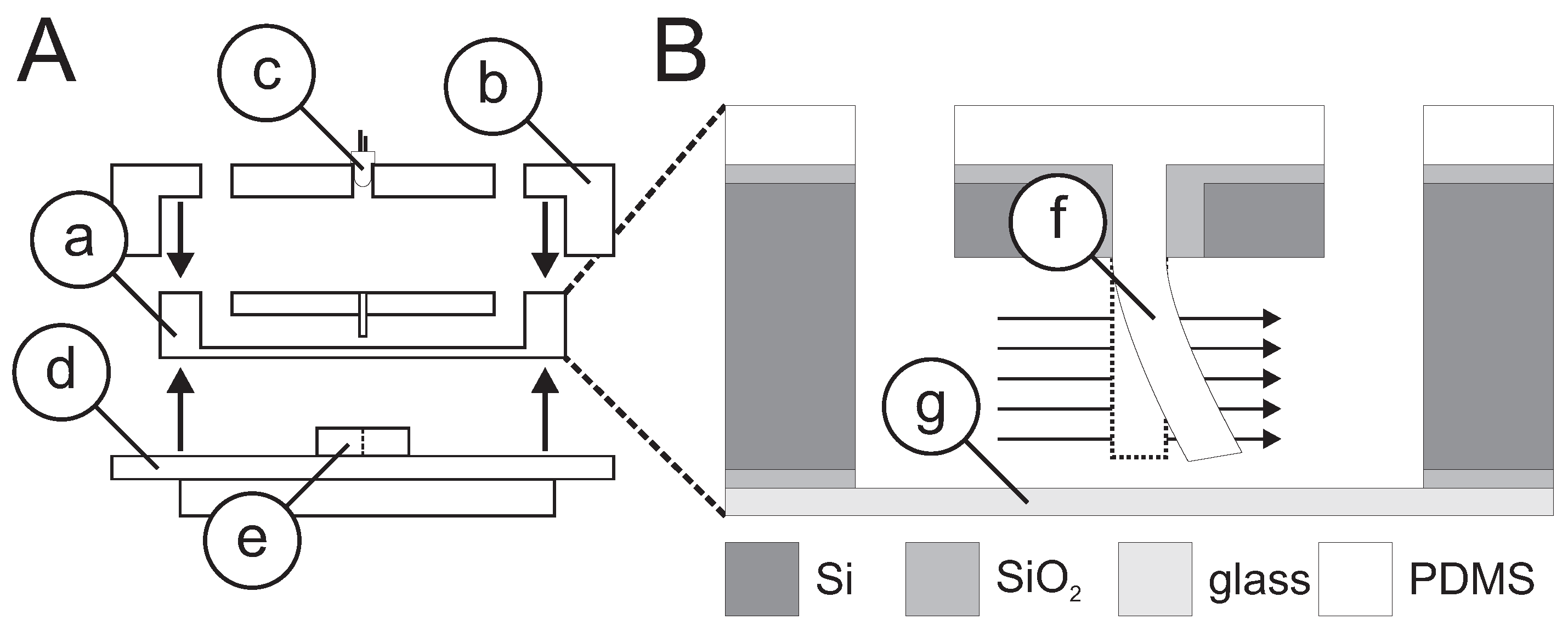
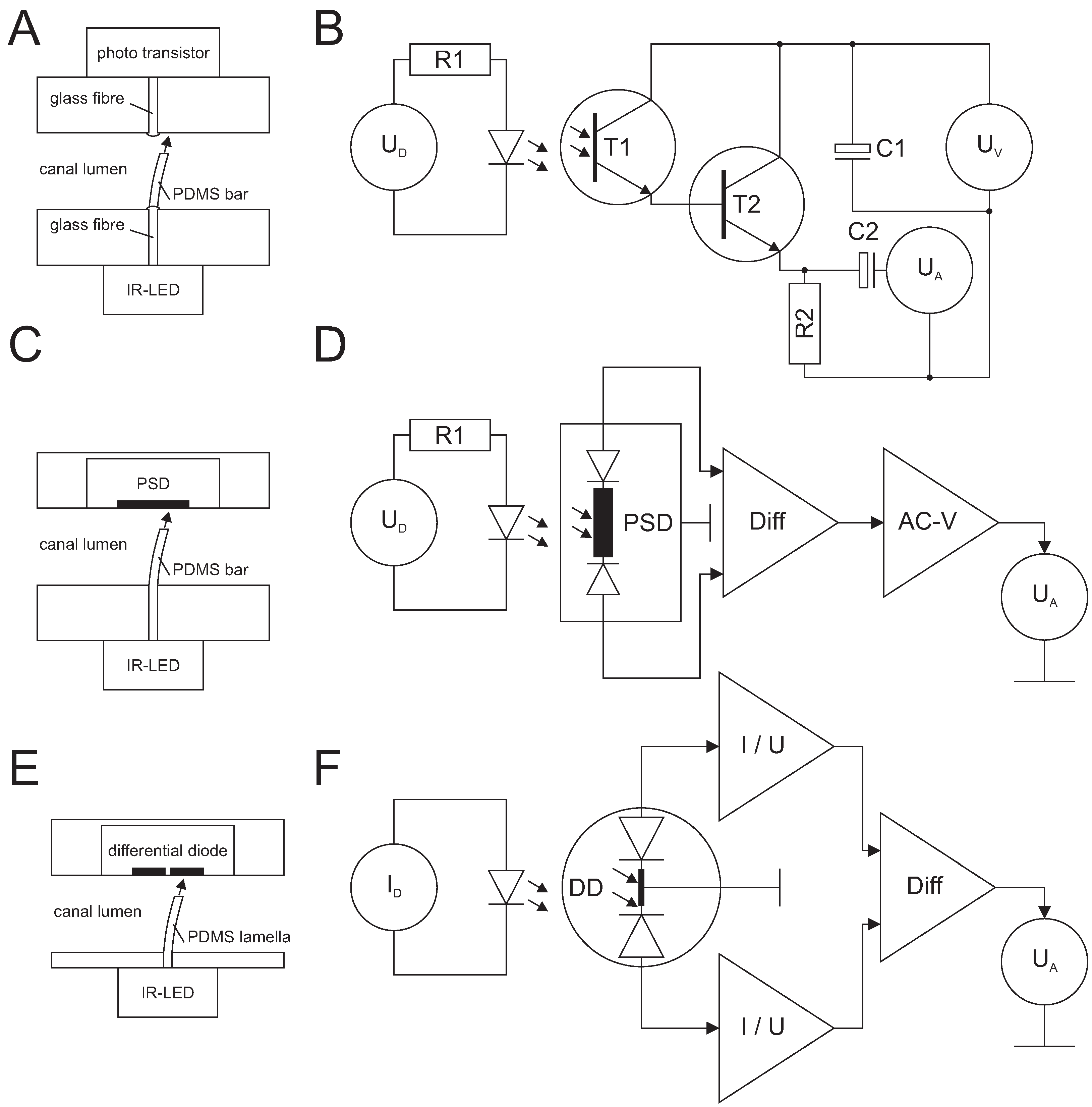
2.1. Biomimetic Transfer: Technical Sensors Based on Canal Neuromasts

Our biomimetic sensor was intended to meter fluid flow in tap water pipelines. Our sensor was exposed to high flow velocities and to particles carried by the stream. Thus, we focused on CNs and took advantage of the high-pass filter properties of lateral line canals to reduce direct current and low frequency fluid flow amplitudes in the canal; previously discussed in [2,6,70,71,72,73]. Beside the reduced flow rate inside the canal due to the bypass configuration of our sensor, small canals offer mechanical protection of the sensory structures that prevents ablation at high flow velocities that may occur in the main stream. Although the canal structure already excludes the contamination of the sensors with particles larger than the canal pores, an additional segregation by means of flexible membranes covering the canal pores may further improve the lifespan of the sensor. Lateral line canals whose pores have a membranous covering also occur in some fish species [20].

We fabricated large-scaled flow sensors using thick-film technology and miniaturized flow sensors using thin-film technology. The sensor based on thick-film technology was fabricated semi-automatically to increase the similarity of the individual lamellae. We used thin-film technology (MEMS) to process deep trenches into the silicon wafer that was used as a casting mold for the sensor lamella. In the second step, the PDMS lamella was vacuum molded and exposed by means of wet etching. A detailed description of the micromachining process and the first verification of the mechanical properties of the sensor are given in [69]. The MEMS sensor featured an aluminum housing for mounting the Si-chip, a glass plate to seal the canal and the read-out electronics (Figure 2).

Figure 2. Assembly of the micro-machined CN. (A) Assembly of the sensory device featuring the Si-chip (a), housing (b), LED (c), electronics PCB (d) with the optical detector (e); (B) magnified Si-chip featuring a PDMS lamella (f) and a glass plate (g). Note that the illustration is not to scale. Modified from [69].

Figure 2. Assembly of the micro-machined CN. (A) Assembly of the sensory device featuring the Si-chip (a), housing (b), LED (c), electronics PCB (d) with the optical detector (e); (B) magnified Si-chip featuring a PDMS lamella (f) and a glass plate (g). Note that the illustration is not to scale. Modified from [69].

In addition to the MEMS process, we adapted the sensor read-out and electronic circuitry to the small dimensions of the sensor lamella. In general, smaller lamellae reduce the sensitivity of the sensor. However, smaller structures have higher resonant frequencies and, thus, can detect higher frequency components, which are presumably present in tap water systems. To compensate for the lower sensitivity, the optical detector and sensor electronics must be chosen carefully.

The read-out principle of our first sensor was in accordance with the light barrier principle (Figure 3A). The lamella was illumined by infrared radiation. The lamella deflection caused a change in light intensity that was detected by the photo transistor. The corresponding electronic circuitry contains only seven parts and amplifies the photo current of the optical detector T1 (Figure 3B; details can be found in [51]). In combination with a large and soft lamella, this read-out technique gives a high sensitivity at low cost. This is true for sensors fabricated by means of thick-film technology. Due to the direct coupling of the electronic devices to the power supply and the lack of compensation for temperature drifts, this simple circuit is not suitable for the much smaller deflections found in the miniaturized lamellae, nor can it be used when direct coupling of the sensor signal is required, e.g., in micro-fluidic applications [69].

The low mechanical sensitivity (deflection) of smaller lamellae was compensated for using optical detectors that were superior to the photo transistor. In the case of the mid-sized lamellae used for the proof of principle, a position sensitive photo diode (PSD) was used in a photo cell configuration (Figure 3C). The lamella deflection induced the motion of a light-spot that was transferred into two output voltages by the PSD. The difference between the voltages leads to a direction sensitive response that was further amplified by means of a capacitive coupled operational amplifier (Figure 3D).

We used a differential photo diode as the readout for the artificial CNs fabricated by means of MEMS techniques (Figure 3E). As the deflection of the lamella was in the micrometer scale, the sensor with the differential photo diode detector had the highest sensitivity. The two sections of this optical detector were placed directly above the resting position of the lamella. The output currents of each of the two sections of the differential photo diode were converted into two voltages by means of a trans-impedance amplifier. A directional sensor output signal was obtained from the differentiation of the output voltages of the trans-impedance amplifiers. Further improvement of the signal-to-noise ratio was achieved by using a low-noise regulation of the current driving the infrared LED (Figure 3F).

Figure 3. Optical read-out principles and sensor electronics. Various sensor read-out principles that were used to detect the deflection of the light-guiding PDMS lamella (left) and corresponding electronic circuits (right). (A) The photo transistor principle uses a Darlington configuration for amplification of the photo transistor current (B) (modified from [51]). (C) The position-sensitive photo diode (PSD) in photo cell operation mode in combination with a voltage subtractor and a capacitive coupled amplifier (D). (E) The differential photo diode (DD) combined with a trans-impedance amplifier followed by a voltage subtractor and a current source used for driving the LED (F).

Figure 3. Optical read-out principles and sensor electronics. Various sensor read-out principles that were used to detect the deflection of the light-guiding PDMS lamella (left) and corresponding electronic circuits (right). (A) The photo transistor principle uses a Darlington configuration for amplification of the photo transistor current (B) (modified from [51]). (C) The position-sensitive photo diode (PSD) in photo cell operation mode in combination with a voltage subtractor and a capacitive coupled amplifier (D). (E) The differential photo diode (DD) combined with a trans-impedance amplifier followed by a voltage subtractor and a current source used for driving the LED (F).

In the proof of principle study presented here, we used a PSD-detector and the voltage differentiator circuit to read-out the mid-sized lamellae built in thick-film technology (Figure 3C,D). For the estimation of bulk flow rates in the tap water metering application, we used micro-machined sensors featuring a differential photo diode and a direct coupled version of the circuit shown in Figure 3D. In the experiments with the separated artificial lateral line canal system, we used a differential photo diode in reverse-voltage operation mode and an operational amplifier in a voltage subtractor configuration. The LED was driven by a current source to regulate the IR radiation intensity.

2.2. Cross-Correlation Flow Metering: Estimated Bulk Flow Rates from Flow Unsteadiness

Fish may estimate bulk flow velocities from the spatial-temporal propagation of flow fluctuations superimposed on the direct current component of bulk water flow [25]. In addition to mimicking fish neuromasts, we also took inspiration from the flow sensing abilities of the fish lateral line for our flow metering principle. Although correlation-based flow meters have been known for some time [74,75,76,77,78,79,80,81], these devices are not yet widely used in every-day applications.

Our work focused on the question of whether bio-inspired arrays mimicking the fish canal system are suitable to perform the flow metering task in pipelines and whether the metering device based on artificial CNs might provide advantages over commercial systems based on ultrasonic or pressure sensors. Previous studies investigated this issue [51,82]. However, experiments were done mainly in open frame flow tanks. As pipelines and water tanks have different hydrodynamic conditions, we tested the applicability of an array of artificial CNs in a pipeline.

Our metering principle is based on the monitoring of local flow fluctuations (pressure and/or flow velocity changes), superimposed on bulk flow, by at least two sensors. Flow fluctuations propagating along the sensor array induce temporally-delayed sensor output signals (upstream sensors detect the flow fluctuation earlier than downstream sensors). The flow velocity is related to the temporal delay of sensor output signals and sensor spacing. The temporal delay between sensor output signals can be estimated by cross-correlation [25,51].

In this study, bulk flow rates were calculated according to Equation (1), where Q is the estimated flow rate, v is the bulk flow velocity, d is the distance between the two sensors, A is the inner cross-section of the metering tube and $\Delta t$ is the temporal offset obtained from a cross-correlation function of the two sensors. Calculated flow rates within a certain velocity range (0 L/h up to twice the maximum flow rate presented) in the experiments (2000 L/h in the proof of principle and 10,000 L/h in the industrial application) were close to the actual flow rates in the pipeline. Values outside the above range were not included in the figures.

$$\begin{array}{cccc}& Q& =A·v=& A·\frac{d}{\Delta t}\end{array}$$

(1)

2.3. Separation of Lateral Line Sensors by Means of Membranes

To separate our artificial CNs from direct contact with the water flow in the pipeline, PDMS membranes were mounted on the aluminum adapter in a set of experiments (Figure 11A). The PDMS membranes, ranging from 10 to 200 µm in thickness, were custom-made by means of a spin coater. The canal structure of our sealed artificial CNs was filled with oil (Leybonol LVO 120, Oerlikon, Switzerland).

3. Results and Discussion

3.1. Proof of Principle: Flow Detection by Cross-Correlation Using an Eight-Fold Sensor Array

We estimated bulk flow velocity in a pipeline by means of a sensory array featuring eight mid-sized lamellae built in thick-film technology (Figure 4A) that were not covered by a membrane. Fluid flow was generated by means of a bilge pump (Model: 355-020-00, SHURflo Ltd., Crawley, UK). The applied flow rates were estimated from the time required to fill a reservoir of 10 L. When water flow was applied to the metering tube, similar waveform shapes featuring a temporal offset were obtained from sensors S4, S5, S6 and S7 (Figure 4B). Due to the not completely automated production process, large variations in sensor sensitivity (e.g., S2 or S8) did occur. Nonetheless, the output signals of four adjacent sensors were suitable for cross-correlation, i.e., for an estimation of bulk flow rates.

Figure 4. Measuring setup and original recording traces obtained in the proof of principle study. (A) Array of eight sensors equipped with mid-sized lamellae built in thick-film technology; (B) The original recording traces of the sensors while stimulated with a bulk flow rate of 672 L/h. Please note that the temporal offsets between similar waveforms from Sensors S4 to S7 (black lines) are also shown in Figure 5. Arrows in (A) indicate flow. Amplitudes are normalized to view the signal shape and are not to scale.

Figure 4. Measuring setup and original recording traces obtained in the proof of principle study. (A) Array of eight sensors equipped with mid-sized lamellae built in thick-film technology; (B) The original recording traces of the sensors while stimulated with a bulk flow rate of 672 L/h. Please note that the temporal offsets between similar waveforms from Sensors S4 to S7 (black lines) are also shown in Figure 5. Arrows in (A) indicate flow. Amplitudes are normalized to view the signal shape and are not to scale.

For higher reference flow rates, such as 797 L/h (Figure 5A) or 672 L/h (Figure 5B), the temporal offset between signals was in the range of the presumed $\Delta t$-values for the reference flow rates applied (see gray bars in Figure 5A–E, which are indicating the expected delays between sensor waveforms). Consequently, the cross-correlation functions showed prominent peaks with high correlation coefficients (Figure 5F,G). Anyway, for lower bulk flow rates, the temporal delay visible in the signals did not match the $\Delta t$-values calculated from the reference flow velocities (Figure 5C,D), although the corresponding cross-correlation functions showed distinct peaks (Figure 5H,I). When no flow was present, the sensor signals were uncorrelated, i.e., the cross-correlation function revealed no prominent peak (Figure 5E,J).

Figure 5. Original signals and cross-correlation functions of the proof of principle study. (A–E) Signals of the adjacent Sensors S6 (gray line) and S7 (black line). Flow rate 797 L/h (A), 672 L/h (B), 485 L/h (C) 308 L/h (D) and 0 L/h (no flow condition) (E). Gray bars indicate expected temporal delay between waveforms. Amplitudes are normalized and not to scale. (F–J) The cross-correlation functions of the two sensor signals shown in (A) to (E) for a time interval of 10 s.

Figure 5. Original signals and cross-correlation functions of the proof of principle study. (A–E) Signals of the adjacent Sensors S6 (gray line) and S7 (black line). Flow rate 797 L/h (A), 672 L/h (B), 485 L/h (C) 308 L/h (D) and 0 L/h (no flow condition) (E). Gray bars indicate expected temporal delay between waveforms. Amplitudes are normalized and not to scale. (F–J) The cross-correlation functions of the two sensor signals shown in (A) to (E) for a time interval of 10 s.

The bulk flow rates estimated from the cross-correlation of adjacent sensor signals (e.g., S4 and S5 or S6 and S7) did not vary over the range of flow rates applied (unfilled circles in Figure 6). In contrast, the flow rates estimated from the cross-correlations of the signals of sensors spaced 10 or 15 mm apart scaled with the reference flow rates applied, even though the sensor array overestimated the real flow rates. When excluding estimated flow rates from adjacent sensors and exceeding the range of 0 to 2000 L/h, the transfer function revealed a linear relation for reference flow rates ranging from 400 to 800 L/h (y = 1.94x − 329.9; R² = 0.76).

Figure 6. Flow rate estimation from temporal delayed waveforms in the proof of principle study. The plot shows the mean values and standard errors for reference flow rates that ranged from 0 to 797 L/h. Sensors were spaced 5 mm apart (open circles, adjacent sensors), 10 mm apart (gray circles) and 15 mm apart (black circles). Data points of estimated flow rates exceeding the range of 0 to 2000 L/h were excluded from this figure (about 35% for adjacent sensors, 25% for 10 mm and 3% for 15 mm sensor distance). Please note that reference values along the x-axis are not equally spaced.

Figure 6. Flow rate estimation from temporal delayed waveforms in the proof of principle study. The plot shows the mean values and standard errors for reference flow rates that ranged from 0 to 797 L/h. Sensors were spaced 5 mm apart (open circles, adjacent sensors), 10 mm apart (gray circles) and 15 mm apart (black circles). Data points of estimated flow rates exceeding the range of 0 to 2000 L/h were excluded from this figure (about 35% for adjacent sensors, 25% for 10 mm and 3% for 15 mm sensor distance). Please note that reference values along the x-axis are not equally spaced.

These results demonstrate that our bio-inspired flow meter can estimate flow rates in pipeline applications. However, we observed some unexpected effects concerning the cross-correlations of the output signals of adjacent sensors. In addition, the estimated flow rates did not match the real flow rates, especially if these were low. It is noteworthy that the estimated flow rates presented here are based on raw data. In future applications, the estimated flow rates can be easily fitted to the real flow rates by the respective transfer function. This holds also true for most other metering devices, such as particle image velocimetry (PIV) recordings or thermal probes, which also need a proper calibration.

In any case, there are basic needs for any metering device: a unique relation between the measured and the reference values, little scattering of the measured values for a given flow velocity and a broad working range. The flow rates obtained in our proof of principle study for the correlation of sensors placed 10 or 15 mm apart show a clear relation to the reference values with little scattering of the derived velocities within the range of 350 to 800 L/h (Figure 6). The transfer function of a sensor should not be mixed up with the calibration of individual sensors. To avoid a costly individual sensor calibration, manufactures aim for a high similarity of metering devices within a production series. Anyway, most tap water flow meters are calibrated routinely to obtain the accuracy needed for tap water flow metering.

3.2. Industrial Application: Flow Measurements in Tap Water Systems

To verify our MEMS-based sensor in an industrial application, we installed the micro-machined version of our bio-inspired metering device in a reference calibration system at the site of our industrial collaborator Hydrometer GmbH (Ansbach, Germany) and applied bulk flow rates similar to those found in ordinary tap water systems that were adjusted by the professional test bench.

The metering device was equipped with three sensors spaced 40 mm apart (Figure 7A). Each sensor chip featured one lamella and was used in a bypass configuration without membranes. When applying flow rates ranging from 200 to about 4000 L/h, the sensors responded to the flow fluctuations in the pipeline (Figure 7B–E). Moreover, our sensor setup withstood pressures of up to six bar, i.e., pressures commonly found in tap water systems. At higher flow rates, adjacent sensors showed similar output signals featuring a temporal offset. For low flow rates, sensor signals contained predominantly noise and hum, indicating that the flow fluctuation was below the threshold (Figure 7F; dynamic properties of sensors built in thin-film technology were examined in [69]).

The cross-correlation functions of all three sensor output signals revealed distinct maxima (Figure 8). Whenever a prominent peak was observed, the corresponding $\Delta t$-values were in good agreement with the presumed temporal offset (Figure 8A–C). However, cross-correlation coefficients were low, indicating a poor similarity of the sensor output signals, especially for low flow rates (Figure 8D).

Whereas the flow rates estimated from adjacent sensors (S1 and S2; S2 and S3) scaled with the reference values, the flow rates derived from the cross-correlation of Sensors S1 and S3 did not (Figure 9). Furthermore, flow rates estimated from adjacent sensor waveforms scaled linearly with the reference flow rates in the range of 500 L/h to about 4000 L/h (y = 0.98x − 157.2; R² = 0.85).

In general terms, our sensory device could be used to estimate flow rates in a tap water system. Further improvement of the metering device with respect to sensitivity and a closer sensor spacing, however, is still desirable. In addition, we used three sensor chips featuring lamellae of varying thickness (50 µm for S1, 35 µm for S2, 25 µm for S3). Lamella dimensions can influence the sensitivity and frequency response of the sensor significantly (see [69] for further details). Thus, varying lamella size and/or shape can be used to increase or shift the dynamic range of flow metering devices that contain several sensors.

However, differences in lamella shape might also reduce the similarity of the sensor signals and, thus, decrease the robustness of the cross-correlations. Since the sensor output signals are normalized by the cross-correlation function, differences in sensor sensitivity had little impact on the cross-correlation results. At higher frequencies, the sensor output signals were phase shifted with respect to the water movements inside the artificial lateral line canal and lead to false $\Delta t$-values. A broad frequency bandwidth of the sensor is beneficial to monitor all kinds of fluctuation that may occur in a pipeline. The cutoff frequencies of our sensors were in the range 30 to 40 Hz (thick-film sensors, [83]) and more than 80 Hz, respectively, for the micro-machined sensors [69]. The flow fluctuations monitored by our sensors were much lower than the high-frequency cutoff frequency of the two sensor types used in the experiments (Figure 4A–E and Figure 7B–F). Therefore, we assume that phase shifts at the high-frequency range had little effects on our metering results.

Figure 7. Setup and output signals of the micro-machined sensors in the tap water metering application. (A) Measuring tube featuring three MEMS sensors (S1, S2 and S3) mounted on adapter plates (see Figure 2). (B–F) The output signals of the three sensors obtained while applying flow rates of 4066 L/h (B), 2550 L/h (C), 1536 L/h (D), 500 L/h (E), and 50 L/h (F). Gray bars indicate expected delay of waveforms.

Figure 7. Setup and output signals of the micro-machined sensors in the tap water metering application. (A) Measuring tube featuring three MEMS sensors (S1, S2 and S3) mounted on adapter plates (see Figure 2). (B–F) The output signals of the three sensors obtained while applying flow rates of 4066 L/h (B), 2550 L/h (C), 1536 L/h (D), 500 L/h (E), and 50 L/h (F). Gray bars indicate expected delay of waveforms.

Figure 8. Cross-correlation (CC) functions of the output signals of the micro-machined sensors in the tap water application. Cross-correlations, each based on two of the micro-machined sensors and a 10 s time interval for the reference velocities of 4066 L/h (A), 2550 L/h (B), 1536 L/h (C), and 500 L/h (D). Arrows indicate temporal offset expected from the reference flow rate applied.

Figure 8. Cross-correlation (CC) functions of the output signals of the micro-machined sensors in the tap water application. Cross-correlations, each based on two of the micro-machined sensors and a 10 s time interval for the reference velocities of 4066 L/h (A), 2550 L/h (B), 1536 L/h (C), and 500 L/h (D). Arrows indicate temporal offset expected from the reference flow rate applied.

Figure 9. Estimated flow rates for reference flow rates ranging from 500 to 4066 L/h. The plot shows mean values and standard errors. Flow rates were estimated from cross-correlations of sensors 1 and 2 (black circles), sensors 2 and 3 (gray circles) and sensors 1 and 3 (open circles) according to Equation (1). Note that estimated flow rates exceeding the range of 0 to 10,000 L/h were excluded from the figure (about 12% for S1 and S2, 8% for S2 and S3, 35% for S1 and S3). Please note that reference values along the x-axis are not equally spaced.

Figure 9. Estimated flow rates for reference flow rates ranging from 500 to 4066 L/h. The plot shows mean values and standard errors. Flow rates were estimated from cross-correlations of sensors 1 and 2 (black circles), sensors 2 and 3 (gray circles) and sensors 1 and 3 (open circles) according to Equation (1). Note that estimated flow rates exceeding the range of 0 to 10,000 L/h were excluded from the figure (about 12% for S1 and S2, 8% for S2 and S3, 35% for S1 and S3). Please note that reference values along the x-axis are not equally spaced.

Our results revealed that under our testing conditions, fluid velocity could barely be estimated for flow velocities below 500 L/h. One prerequisite for an accurate calibration of the conventional turbine flow meters of our collaborator is laminar flow. As a consequence, the testing bench was designed such that fluid flow inside the pipeline was highly laminar. Since our metering principle is based on the detection of flow fluctuations, the low turbulence levels found especially at low flow velocities might be one of the reasons why we failed to measure low flow velocities. We suggest that a small cylinder placed upstream from the metering device will improve the metering performance. In the measurements with the sensors produced in thick-film technology, we used a bilge pump and a flexible tube of about 1 m in length for flow generation. We assume that this pump generated turbulent flow that led to a stronger stimulation of the flow sensors. In addition, the larger scale sensors had a higher sensitivity to alternating pressure signals [68,69]. Thus, the detection threshold of the larger sensors most likely was reduced due to the turbulences and the higher sensitivity of these sensors.

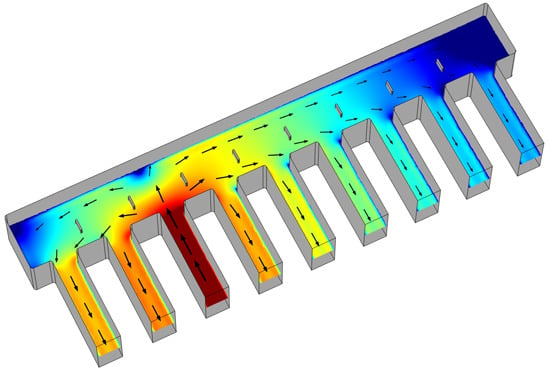
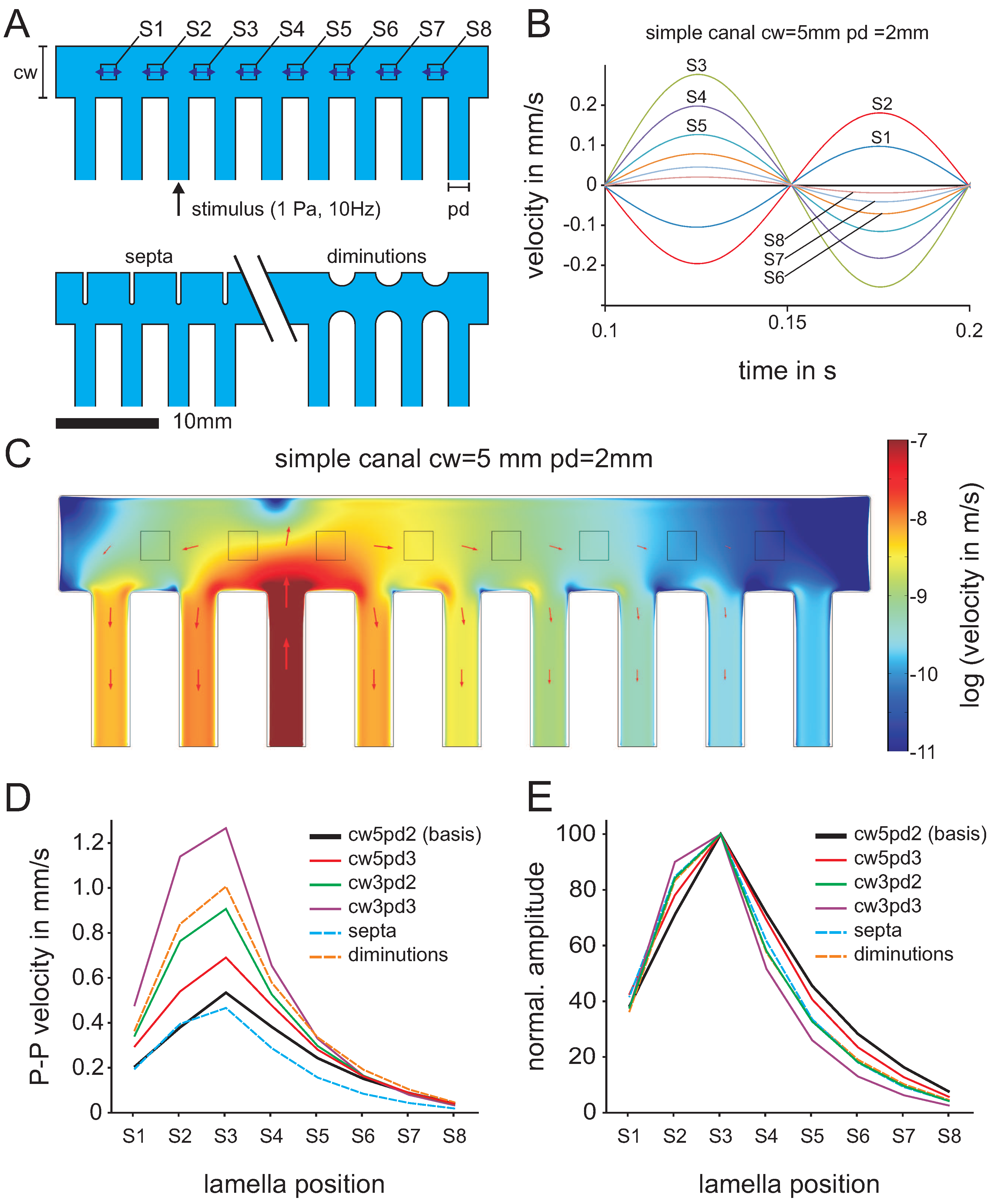
3.3. Influence of Canal Properties on Flow Metering: A FEM Study

Our results raised some questions, e.g., about the influence of canal shape on the flow rates measured. We found seemingly contradicting results in the proof of principle study using the sensor array featuring larger lamellae built in thick-film technology and the industrial application using the micro-machined flow sensors. Whereas in the proof of principle study, cross-correlations obtained from adjacent sensors did not reveal the correct flow rates, in the industrial application study, only the output signals from adjacent sensors led to useful cross-correlation results.

Thus, we used finite element modeling (COMSOL Multiphysics, Version 4.2, laminar flow, time depending study) to quantify the fluid flow inside canal systems. The simulation is based on a 2D-model of the eight-fold sensory array used in our proof of principle study (Figure 10A). The canal width (cw) was 5 mm; the pore diameter (pd) was 2 mm. Due to the high flexibility of the PDMS and the high computational effort, our simplified simulation did not use deformable lamellae. Instead, the average flow velocity inside the canal was calculated at the spots were the lamellae were located in the real sensor (S1 to S8 in Figure 10A). In the simulation, a sinusoidal pressure signal (10 Hz, 1 Pa) applied to the third pore of the canal (Figure 10A) mimicked flow fluctuations in a real pipeline. All other canal pores were pressure outlets (0 Pa). When pressure fluctuations were applied, sinusoidal fluid motions were induced at the lamella positions S1 to S8 (Figure 10B). The spatial distribution of the fluid flow revealed complex flow patterns inside the canal structure (Figure 10C). In general, a gradient in fluid velocity was found between the positions S3 and S4 and the other sensors (e.g., S7 and S8 in Figure 10B,C). As a consequence, only small differences in flow velocity were found between closely-spaced sensors (e.g., about 80% for sensor positions S3 and S4; the black line in Figure 10D).

In the next step, we modified the canal structure in our simulations and verified how this affects the flow in the artificial canal. In the simulations, we changed canal width and pore dimensions. In addition, we inserted diminutions or septa to build more complex canals (Figure 10A). Thereafter, we calculated the flow velocities at the eight sensor positions and compared these velocities with the velocities calculated for the “basic canal” (simple canal shape, canal width 5 mm, pore dimension 2 mm; labeled “cw5pd2”; black line in Figure 10D,E). For our simulations, we used a simple canal with 3-mm pores (cw5pd3; red line in Figure 10D,E), simple canals with a canal width of 3 mm (cw3pd2; green line in Figure 10D,E) and simple canals with a width and pore size of 3 mm (cw3pd3; purple line in Figure 10D,E). Furthermore, we added septa with a width of about 3.1 mm (blue dashed line in Figure 10D,E) and diminutions with a width of about 1.3 mm (orange dashed line in Figure 10D,E) to the main canal, but kept the pore dimension at 2 mm and the canal width at 5 mm (maximal diameter; diminutions and septa decreased the canal width at certain positions; see the lower part of Figure 10A). Please note that pictures of a higher resolution and animations of fluid flow inside the canal systems are provided as Supplementary Information.

Figure 10. Finite element simulation of mechanical cross-talk induced by the canal geometry. (A) Simple canals (top) with variable canal widths (cw) and pore dimensions (pd). Complex canals included septa or diminutions (below). Fluid flow was examined at locations S1 to S8 when stimulated with alternating pressure of 1 Pa at 10 Hz. (B) The velocity components in the horizontal direction at locations S1 to S8 (see the double-headed arrows in (A)). The colors of the curves do not correspond to the colors in (D)/(E). (C) The flow field inside the basic canal in logarithmic scaling (see also Figure 4A). (D) Peak-to-peak amplitudes at locations S1 to S8 for various canal shapes and dimensions (shown in (A)) (E) Normalized peak-to-peak amplitudes from (D), referenced to the velocity at location S3.

Figure 10. Finite element simulation of mechanical cross-talk induced by the canal geometry. (A) Simple canals (top) with variable canal widths (cw) and pore dimensions (pd). Complex canals included septa or diminutions (below). Fluid flow was examined at locations S1 to S8 when stimulated with alternating pressure of 1 Pa at 10 Hz. (B) The velocity components in the horizontal direction at locations S1 to S8 (see the double-headed arrows in (A)). The colors of the curves do not correspond to the colors in (D)/(E). (C) The flow field inside the basic canal in logarithmic scaling (see also Figure 4A). (D) Peak-to-peak amplitudes at locations S1 to S8 for various canal shapes and dimensions (shown in (A)) (E) Normalized peak-to-peak amplitudes from (D), referenced to the velocity at location S3.

In relation to the basic canal shape, an increase of average flow velocity was found in all canal shapes with the exception of the complex canal featuring septa (Figure 10D; red, green, purple and orange dashed lines are above the bold black line which represents the basic canal). The increase in flow velocity was most prominent close to the pore stimulated (e.g., S2, S3 and S4). As a consequence, the modification of the canal shape increased the overall sensitivity of the sensor. In the case of the complex canal with the septa, a decrease in flow velocity was found for sensors S3 to S8.

To compare the crosstalk performance of the different canal shapes, the flow velocity amplitudes were normalized with respect to the flow velocity at S3. This comparison revealed lower relative flow velocities in all alternative canal shapes at the sensor positions S4 to S8. Thus, crosstalk between sensors S3 to S8 was reduced by these canal modifications. Anyway, the modification of the canal shape did not reduce the relative amplitudes at the sensor positions S1 and S2.

In our industrial application study, mechanical crosstalk was avoided by using several sensor chips, each featuring only one lamella. The downside of this configuration was that sensor spacing increased from 5 to 40 mm. The larger distance between sensors S1 and S3 (80 mm) might be the reason for the lower similarity of the sensor output signals. Small differences in size and shape of the lamellae might also have contributed to this effect.

Nonetheless, the canal used in the finite element modeling (FEM) was a simplified version of the real prototype (2D simulation, no deflectable lamellae, only one pore stimulated, only one sine wave signal). Due to the frequency response of lateral line canals, our simulations do not reflect every detail of the complex fluid flow in real lateral line canals. In further experiments, an experimental investigation of canals that differ in size and shape will allow us to verify the results of our simulations. These investigations may also help us to better understand the functional significance of the diversity of fish lateral line canals (“reverse” bio-mimetics).

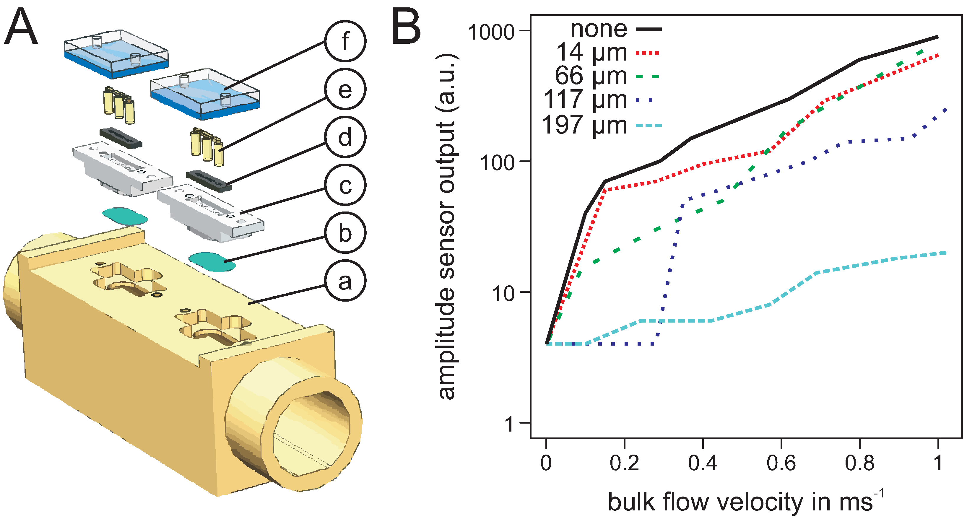
3.4. A Segregated Artificial Lateral Line: Medical and Pharmaceutical Applications

Fluid separation is a prerequisite for any medical application, e.g., to prevent contamination of the measuring system with blood or other body fluids. We sealed our artificial CNs with thin membranes and filled the canal structure with mineral oil (Figure 11A). Thereafter, we verified whether the fluctuations superimposed on bulk water flow can still be detected. Compared to still water condition (0 m/s), amplitudes of the sensor output signals increased when bulk water flow was present in the pipeline. This was true for most of the membranes and velocities tested (Figure 11B). Thus, the flow fluctuations in the pipeline were still detectable even when the canal pores were covered with PDMS membranes. Thick membranes reduced the amplitude of the sensor output signals. In addition, sensor signals were only obtained at higher bulk flow velocities. Thus, sealing the pores of the canals with thick PDMS membranes shifted the detection threshold of the flow metering device to higher bulk flow rates.

Canals were not only filled with water, but also with mineral oil. Since water and mineral oil differ, e.g., in density (lower for oil than for water), viscosity (mineral oil about 100 times higher) and fraction index (about 1.5 for mineral oil and 1.3 for water), we can expect that the two different fluids lead to different frequency responses of the sealed sensors. This should be investigated in more detail in further studies.

Figure 11. Verification of an artificial CN sealed with a PDMS membrane by flow-induced fluctuations. (A) Schematic drawing of the sensor setup featuring a metering tube (a), a PDMS membrane (b), an aluminum adapter with pores (c), a Si-chip with lamellae (d), mineral oil filling (e) and sealed read-out electronics (f); (B) Output signals of a sensor with open pores and with pores covered by different PDMS membranes (thicknesses of 14, 66, 117 and 197 µm). Bulk flow velocities varied from 0 to 1 m/s.

Figure 11. Verification of an artificial CN sealed with a PDMS membrane by flow-induced fluctuations. (A) Schematic drawing of the sensor setup featuring a metering tube (a), a PDMS membrane (b), an aluminum adapter with pores (c), a Si-chip with lamellae (d), mineral oil filling (e) and sealed read-out electronics (f); (B) Output signals of a sensor with open pores and with pores covered by different PDMS membranes (thicknesses of 14, 66, 117 and 197 µm). Bulk flow velocities varied from 0 to 1 m/s.

4. Conclusions

In this study, we used two setups featuring bio-mimetic flow sensors to monitor the propagation of flow fluctuations in a pipeline. Bulk flow rates were calculated from the temporal delay found in the waveforms of the sensors within an array. The estimated bulk flow rates scaled with the reference flow rates applied. Thus, we showed the suitability of artificial CNs for applications like tap water flow metering. However, both sensor setups still must be further improved with respect to a broader dynamic range, especially at the lower velocity end.

The results of the FEM revealed that the output signals of neighboring sensors can only be used for the calculation of flow velocity for certain canal shapes (see also [70,71,84,85]; see [86] for sensory hairs of cricket cerci). In our proof of principle study, the larger lamellae produced in thick-film technology were located in one wide “end-to-end main canal structure” featuring small pores. Pressure fluctuations acting on one pore can spread inside the canal and, thus, can stimulate the lamellae of all artificial neuromasts. According to our simulations and in agreement with the experimental results, increasing lamellae distance reduces mechanical crosstalk. In addition, the FEM simulations show that crosstalk between neighboring sensors can be reduced by decreasing the canal width and/or by increasing the pore dimension. The crosstalk between adjacent sensors can also be reduced by building complex canals that feature septa or diminutions. Altering canal dimension also alters sensor sensitivity. In our simulations, the 3 mm wide canal with the 3 mm pores was most sensitive. Thus, canals with a diameter of 3 mm and a pore size of 3 mm are a good starting point for further optimization of metering devices.

The sealing experiments revealed that our artificial CNs still detect flow fluctuations, when the pores of the sensor are sealed by PDMS membranes. Thin membranes had a smaller effect on the flow fluctuation-induced sensor output signal. Membrane thickness of more than 100 µm were not suitable for the detection of flow fluctuations, at least in our sensor setup.

Future prospects include a further characterization of the sensors in terms of long-term stability of the lamellae, electronics and the sealing, as well as environmental aspects, like biological fouling, and continued optimization of the fabrication process. Further experiments will also address the performance of the sealed artificial CNs regarding the estimation of flow rates in accordance with the cross-correlation principle. In addition, we will focus on the automated membrane fabrication and the automated filling of the artificial canal system. This will be beneficial in terms of reproducibility and also sterilization of a sensor device relevant to the healthcare sector.

References

1. Dijkgraaf, S. The functioning and significance of the lateral-line organs. Biol. Rev. 1962, 38, 51–105. [Google Scholar] [CrossRef]
2. Coombs, S. Smart Skins: Information Processing by Lateral Line Flow Sensors. Autono. Robot. 2001, 11, 255–261. [Google Scholar] [CrossRef]
3. Coombs, S.; New, J.G.; Nelson, M. Information-processing demands in electrosensory and mechanosensory lateral line systems. J. Physiol. Paris 2002, 96, 341–354. [Google Scholar] [CrossRef]
4. Bleckmann, H. Peripheral and central processing of lateral line information. J. Comp. Physiol. A 2008, 194, 145–158. [Google Scholar] [CrossRef] [PubMed]
5. Bleckmann, H.; Klein, A.; Meyer, G. Nature as a model for technical sensors. In Frontiers in Sensing; Springer: Wien, Austria, 2012; pp. 3–18. [Google Scholar]
6. Montgomery, J.; Coombs, S.; Halstead, M. Biology of the mechanosensory lateral line in fishes. Rev. Fish Biol. Fish. 1995, 5, 399–416. [Google Scholar] [CrossRef]
7. Montgomery, J.C.; McDonald, F.; Baker, C.F.; Carton, A.G.; Ling, N. Sensory integration in the hydrodynamic world of rainbow trout. Proc. R. Soc. Lond. Ser. B 2003, 270, 195–197. [Google Scholar] [CrossRef] [PubMed]
8. Schmitz, A.; Bleckmann, H.; Mogdans, J. Organization of the Superficial Neuromast System in Goldfish, Carassius auratus. J. Morphol. 2008, 269, 751–761. [Google Scholar] [CrossRef] [PubMed]
9. Dijkgraaf, S. Untersuchungen über die Funktion der Seitenlinienorgane an Fischen. Z. Physiol. 1933, 20, 162–214. (In German) [Google Scholar]
10. Flock, Å. Electronmicroscopic and electrophysiological studies on the lateral line canal organ. Acta Otolaryngol. 1965, 199, 1–90. [Google Scholar]
11. Hudspeth, A.J.; Corey, D.P. Sensitivity, polarity, and conductance change in the response of vertebrate hair cells to controlled mechanical stimuli. Proc. Natl. Acad. Sci. USA 1977, 74, 2407–2411. [Google Scholar] [CrossRef] [PubMed]
12. Hudspeth, A.J. Mechanoelectrical transduction by hair cells in the acousticolateralis sensory system. Ann. Rev. Neurosci. 1983, 6, 187–215. [Google Scholar] [CrossRef] [PubMed]
13. Kroese, A.; van Netten, S. Sensory Transduction in lateral line hair cells. In The Mechanosensory Lateral Line: Neurobiology and Evolution; Coombs, S., Görner, P., Münz, H., Eds.; Springer: New York, NY, USA, 1989; pp. 265–284. [Google Scholar]
14. Yamada, Y.; Hama, K. Fine Structure of the Lateral-Line Organ of the Common Eel, Anguilla japonica. Z. Zellforsch. 1972, 124, 454–464. [Google Scholar] [CrossRef] [PubMed]
15. Hama, K.; Yamada, Y. Fine Structure of the Ordinary Lateral Line Organ II. The Lateral Line Canal Organ of Spotted Shark, Mustelus manazo. Cell Tissue Res. 1977, 176, 23–36. [Google Scholar] [PubMed]
16. Hama, K.M. Some observations on the fine structure of the lateral line organ of the Japanese sea eel Lyncozymba nystromi. J. Cell Biol. 1965, 24, 193–210. [Google Scholar] [CrossRef] [PubMed]
17. Görner, P. Untersuchungen zur Morphologie und Elektrophysiologie des Seitenlinienogans vom Krallenfrosch (Xenopus Laevis Daudin). Z. Vergleichende Physiol. 1963, 47, 316–338. (In German) [Google Scholar] [CrossRef]
18. Bauknight, R.; Strelioff, D.; Honrubia, V. Effective stimulus for the Xenopus laevis lateral-line hair-cell system. Laryngoscope 1976, 86, 1836–1844. [Google Scholar] [CrossRef] [PubMed]
19. Faucherre, A.; Pujol-Martí, J.; Kawakami, K.; López-Schier, H. Afferent Neurons of the Zebrafish Lateral Line Are Strict Selectors of Hair-Cell Orientation. PLoS ONE 2009, 4, e4477. [Google Scholar] [CrossRef] [PubMed]
20. Coombs, S.; Janssen, J.; Webb, J. Diversity of lateral line systems: Evolutionary and functional considerations. In Sensory Biology of Aquatic Animals.; Atema, J., Fay, R.R., Popper, A.N., Tavolga, W.N., Eds.; Springer: New York, NY, USA, 1988; pp. 553–593. [Google Scholar]
21. Kroese, A.B.A.; Schellart, N.A.M. Velocity- and Acceleration-Sensitive Units in the Trunk Lateral Line of the Trout. J. Neurophysiol. 1992, 68, 2212–2221. [Google Scholar] [PubMed]
22. Kalmijn, A. Hydrodynamic and acoustic field detection. In Sensory Biology of Aquatic Animals; Springer: New York, NY, USA, 1988; pp. 151–186. [Google Scholar]
23. Coombs, S.; Montgomery, J.C. The enigmatic lateral line system. In Comparative Hearing: Fish and Amphibians; Springer: New York, NY, USA, 1999; pp. 319–362. [Google Scholar]
24. Chagnaud, B.P.; Bleckmann, H.; Hofmann, M.H. Lateral line nerve fibers do not code bulk water flow direction in turbulent flow. Zoology 2008, 111, 204–217. [Google Scholar] [CrossRef] [PubMed]
25. Chagnaud, B.P.; Brücker, C.; Hofmann, M.H.; Bleckmann, H. Measuring Flow Velocity and Flow Direction by Spatial and Temporal Analysis of Flow Fluctuations. J. Neurosci. 2008, 28, 4479–4487. [Google Scholar] [CrossRef] [PubMed]
26. Voth, G.A.; La Porta, A.; Crawford, A.M.; Alexander, J.I.M.; Bodenschatz, E. Measurement of particle accelerations in fully developed turbulence. J. Fluid Mech. 2002, 469, 121–160. [Google Scholar] [CrossRef]
27. Barth, S.; Koch, H.; Kittel, A.; Peinke, J.; Burgold, J.; Wurmus, H. Laser-cantilever anemometer: A new high-resolution sensor for air and liquid flows. Rev. Sci. Instrum. 2005, 76, 075110. [Google Scholar] [CrossRef]
28. Yang, Y.; Chen, J.; Engel, J.; Pandya, S.; Chen, N.; Tucker, C.; Coombs, S.; Jones, D.L.; Liu, C. Distant touch hydrodynamic imaging with an artificial lateral line. Proc. Nal. Acad. Sci. USA 2006, 103, 18891–18895. [Google Scholar] [CrossRef] [PubMed]
29. Chen, Z.; Shen, Y.; Xi, N.; Tan, X. Integrated sensing for ionic polymer-metal composite actuators using PVDF thin films. Smart Mater. Struct. 2007, 16, 262–271. [Google Scholar] [CrossRef]
30. Toschi, F.; Bodenschatz, E. Lagrangian Properties of Particles in Turbulence. Annual Rev. Fluid Mech. 2009, 41, 375–404. [Google Scholar] [CrossRef]
31. Zhang, Y.; Tadigadapa, S.; Najafi, N. A micromachined Coriolis-force-based mass flowmeter for direct mass flow and fluid density measurements. Transducers 2001, 1, 1460. [Google Scholar]
32. Mogdans, J.; Engelmann, J.; Hanke, W.; Kröther, S. The Fish Lateral Line: How to Detect Hydrodynamic Stimuli. In Sensors and Sensing in Biology and Engineering; Springer: New York, NY, USA, 2003; pp. 173–185. [Google Scholar]
33. Colgate, J.E.; Lynch, K.M. Mechanics and Control of Swimming: A Review. IEEE J. Ocean. Eng. 2004, 29, 660–673. [Google Scholar] [CrossRef]
34. Yang, Y.; Nguyen, N.; Chen, N.; Lockwood, M.; Tucker, C.; Hu, H.; Bleckmann, H.; Liu, C.; Jones, D.L. Artificial lateral line with biomimetic neuromasts to emulate fish sensing. Bioinspir. Biomim. 2010, 5, 1–9. [Google Scholar] [CrossRef] [PubMed]
35. Bogue, R. Inspired by nature: Developments in biomimetic sensors. Sens. Rev. 2009, 29, 107–111. [Google Scholar]
36. Goulet, J.; Engelmann, J.; Chagnaud, B.P.; Franosch, J.M.P.; Suttner, M.D.; van Hemmen, J.L. Object localization through the lateral line system of fish: theory and experiment. J. Comp. Physiol. A 2008, 194, 1–17. [Google Scholar] [CrossRef] [PubMed]
37. Yan, G.H.; Chen, Z.F.; Sun, J.C. Using a linear array to estimate the velocity of underwater moving targets. J. Mar. Sci. Appl. 2009, 8, 343–347. [Google Scholar] [CrossRef]
38. Asadnia, M.; Kottapalli, A.G.P.; Shen, Z.; Miao, J.; Triantafyllou, M. Flexible and surface-mountable piezoelectric sensor arrays for underwater sensing in marine vehicles. IEEE Sens. J. 2013, 13, 3918–3925. [Google Scholar] [CrossRef]
39. Peleshanko, S.; Julian, M.D.; Ornatska, M.; McConney, M.E.; LeMieux, M.C.; Chen, N.; Tucker, C.; Yang, Y.; Liu, C.; Humphrey, J.A.C.; et al. Hydrogel-Encapsulated Microfabricated Haircells Mimicking Fish Cupula Neuromast. Adv. Mater. 2007, 19, 2903–2909. [Google Scholar] [CrossRef]
40. Liu, C. Micromachined biomimetic artificial haircell sensors. Bioinspir. Biomim. 2007, 2, S162–S169. [Google Scholar] [CrossRef] [PubMed]
41. McConney, M.E.; Chen, N.; Lu, D.; Hu, H.A.; Coombs, S.; Liu, C.; Tsukruk, V.V. Biologically inspired design of hydrogel-capped hair sensors for enhanced underwater flow detection. Soft Matter 2009, 5, 292–295. [Google Scholar] [CrossRef]
42. Su, Y.; Evans, A.G.R.; Brunnschweiler, A.; Ensell, G. Characterization of a highly sensitive ultra-thin piezoresistive silicon cantilever probe and its application in gas flow velocity sensing. J. Micromech. Microeng. 2002, 12, 780–785. [Google Scholar] [CrossRef]
43. Chen, N.; Tucker, C.; Engel, J.M.; Yang, Y.; Pandya, S.; Liu, C. Design and Characterization of Artificial Haircell Sensor for Flow Sensing with Ultrahigh Velocity and Angular Sensitivity. J. Microelectromech. Syst. 2007, 16, 999–1014. [Google Scholar] [CrossRef]
44. Dijkstra, M.; van Baar, J.J.; Wiegerink, R.J.; Lammerink, T.S.J.; de Boer, J.H.; Krijnen, G.J.M. Artificial sensory hairs based on the flow sensitive receptor hairs of crickets. J. Micromech. Microeng. 2005, 15, 132–138. [Google Scholar] [CrossRef]
45. Krijnen, G.J.M.; Dijkstra, M.; van Baar, J.J.; Shankar, S.S.; Kuipers, W.J.; de Boer, R.J.H.; Altpeter, D.; Lammerink, T.S.J.; Wiegerink, R. MEMS based hair flow-sensors as model systems for acoustic perception studies. Nanotechnology 2006, 17, 84–89. [Google Scholar] [CrossRef] [PubMed]
46. Izadi, N.; de Boer, M.; Berenschot, J.; Wiegerink, R.; Lammerink, T.; Jansen, H.; Mogdans, J.; Krijnen, G. Fabrication of dense flow sensor arrays on flexible membranes. In Proceedings of the International Solid-State Sensors, Actuators and Microsystems Conference, Denver, CO, USA, 21–25 June 2009; pp. 1075–1078.
47. Abdulsadda, A.T.; Tan, X. An artificial lateral line system using IPMC sensor arrays. Int. J. Smart Nano Mater. 2012, 3, 226–242. [Google Scholar] [CrossRef]
48. Große, S.; Schröder, W.; Brücker, C. Nano-newton drag sensor based on flexible micro-pillars. Meas. Sci. Technol. 2006, 17, 2689–2697. [Google Scholar] [CrossRef]
49. Brücker, C.; Bauer, D.; Chaves, H. Dynamic response of micro-pillar sensors measuring fluctuating wall-shear-stress. Exp. Fluids 2007, 42, 737–749. [Google Scholar] [CrossRef]
50. Lien, V.; Vollmer, F. Microfluidic flow rate detection based on integrated optical fiber cantilever. Lab Chip 2007, 7, 1352–1356. [Google Scholar] [CrossRef] [PubMed]
51. Klein, A.T.; Bleckmann, H. Determination of object position, vortex shedding frequency and flow velocity using artificial lateral line canals. Beilstein J. Nanotechnol. 2011, 2, 276–283. [Google Scholar] [CrossRef] [PubMed]
52. McConney, M.E.; Anderson, K.D.; Brott, L.L.; Naik, R.R.; Tsukruk, V.V. Bioinspired Material Approaches to Sensing. Adv. Funct. Mater. 2009, 19, 2527–2544. [Google Scholar] [CrossRef]
53. Fan, Z.; Chen, J.; Zou, J.; Bullen, D.; Liu, C.; Delcomyn, F. Design and fabrication of artificial lateral line flow sensors. J. Micromech. Microeng. 2002, 12, 655–661. [Google Scholar] [CrossRef]
54. Qualtieri, A.; Rizzi, F.; Todaro, M.; Passaseo, A.; Cingolani, R.; Vittorio, M.D. Stress-driven AlN cantilever-based flow sensor for fish lateral line system. Microelectron. Eng. 2011, 88, 2376–2378. [Google Scholar] [CrossRef]
55. Qualtieri, A.; Rizzi, F.; Epifani, G.; Ernits, A.; Kruusmaa, M.; Vittorio, M.D. Parylene-coated bioinspired artificial hair cell for liquid flow sensing. Microelectron. Eng. 2012, 98, 516–519. [Google Scholar] [CrossRef]
56. Tang, L.; Zhang, K.; Chen, S.; Zhang, G.; Liu, G. MEMS inclinometer based on a novel piezoresistor structure. Microelectron. J. 2009, 40, 78–82. [Google Scholar] [CrossRef]
57. Xue, C.; Chen, S.; Zhang, W.; Zhang, B.; Zhang, G.; Qiao, H. Design, fabrication, and preliminary characterization of a novel MEMS bionic vector hydrophone. Microelectron. J. 2007, 38, 1021–1026. [Google Scholar] [CrossRef]
58. Zhang, G.; Wang, P.; Guan, L.; Xiong, J.; Zhang, W. Improvement of the MEMS bionic vector hydrophone. Microelectron. J. 2011, 42, 815–819. [Google Scholar] [CrossRef]
59. Fernandez, V.I.; Hou, S.M.; Hover, F.S.; Lang, J.H.; Triantafyllou, M.S. Lateral-Line-Inspired MEMS-Array Pressure Sensing for Passive Underwater Navigation; Sea Grant College Program; Massachusetts Institiute of Technology: Cambridge, MA, USA, 2007. [Google Scholar]
60. Ozaki, Y.; Yasuda, T.; Shimoyama, I. An Air flow Sensor Modeled on Wind Receptor Hairs of Insects. In Proceedings of the 13th Annual International Conference on Micro Electro Mechanical Systems (MEMS 2000), Miyazaki, Japan, 23–27 January 2000; pp. 531–536.
61. Krijnen, G.J.M.; Lammerink, T.; Wiegerink, R.; Casas, J. Cricket Inspired Flow-Sensor Arrays. In Proceedings of 2007 IEEE on Sensors, Atlanta, GA, USA, 28-31 October 2007; pp. 539–546.
62. Izadi, N.; de Boer, M.; Berenschot, J.; Krijnen, G. Fabrication of superficial neuromast inspired capacitive flow sensors. J. Micromechan. Microeng. 2010, 20, 085041. [Google Scholar] [CrossRef]
63. Abdulsadda, A.T.; Tan, X. Nonlinear estimation-based dipole source localization for artificial lateral line systems. Bioinspir. Biomim. 2013, 8, 2005–2019. [Google Scholar] [CrossRef] [PubMed]
64. Abdulsadda, A.T.; Tan, X. Underwater tracking of a moving dipole source using an artificial lateral line: Algorithm and experimental validation with ionic polymer-metal composite flow sensors. Smart Mater. Struct. 2013, 22, 045010. [Google Scholar] [CrossRef]
65. Ganley, T.; Hung, D.L.S.; Zhu, G.; Tan, X. Modeling and Inverse Compensation of Temperature-Dependent Ionic Polymer-Metal Composite Sensor Dynamics. IEEE/ASME Trans. Mechatron. 2011, 16, 80–89. [Google Scholar] [CrossRef]
66. Lei, H.; Lim, C.; Tan, X. Modeling and inverse compensation of dynamics of base-excited ionic polymer-metal composite sensors. J. Intell. Mater. Syst. Struct. 2013, 24, 1557–1571. [Google Scholar] [CrossRef]
67. Klein, A.T.; Herzog, H.; Bleckmann, H. Lateral line canal morphology and signal to noise ratio. In Proceedings of the SPIE Smart Structures and Materials+ Nondestructive Evaluation and Health Monitoring, San Diego, CA, USA, 6 March 2011.
68. Klein, A.T.; Münz, H.; Bleckmann, H. The functional significance of lateral line canal morphology on the trunk of the marine teleost Xiphister atropurpureus (Stichaeidae). J. Comp. Physiol. A 2013, 199, 735–749. [Google Scholar] [CrossRef] [PubMed]
69. Herzog, H.; Klein, A.T.; Bleckmann, H.; Holik, P.; Schmitz, S.; Siebke, G.; Tätzner, S.; Lacher, M.; Steltenkamp, S. μ-biomimetic flow sensors—Introducing light-guiding PDMS structures into MEMS. Bioinspir. Biomim. 2015, 10, 036001. [Google Scholar] [CrossRef] [PubMed]
70. Barbier, C.; Humphrey, J.A. Drag force acting on a neuromast in the fish lateral line trunk canal. I. Numerical modelling of external -internal flow coupling. J. R. Soc. Interface 2009, 6, 627–640. [Google Scholar] [PubMed]
71. Humphrey, J.A. Drag force acting on a neuromast in the fish lateral line trunk canal. II. Analytical modelling of parameter dependencies. J. R. Soc. Interface 2009, 6, 641–653. [Google Scholar] [CrossRef] [PubMed]
72. Denton, E.J.; Gray, J. Mechanical Factors in the Excitation of Clupeid Lateral Lines. Proc. R. Soc. Lond. Ser. B 1983, 218, 1–26. [Google Scholar] [CrossRef]
73. Denton, E.; Gray, J. Some Observations on the Forces Acting on Neuromasts in Fish Lateral Line Canals. In The Mechanosensory Lateral Line: Neurobiology and Evolution; Coombs, S., Görner, P., Münz, H., Eds.; Springer: New York, NY, USA, 1989; pp. 229–246. [Google Scholar]
74. Sheen, S.; Raptis, A. Acoustic Cross-Correlation Flowmeter for Solid-Gas Flow. U.S. Patent 4,598,593, 8 July 1986. [Google Scholar]
75. Amemiya, S. Correlation Detection Type Ultrasound Blood Flowmeter. U.S. Patent 4,693,319, 15 September 1987. [Google Scholar]
76. Inada, Y.; Sugimoto, K. Cross Correlation Flowmeter. U.S. Patent 4,841,780, 27 June 1989. [Google Scholar]
77. Margit, B.; Joerg, R.; Frank, S. Ultrasound Flowmeter Which Functions according to the Delay Correlation Method. DE Patent 19,815,199, 14 October 1999. [Google Scholar]
78. Veneruso, A.; Huang, S. Cross Correlation Fluid Flow Meter. U.S. Patent 5,948,995, 7 September 1999. [Google Scholar]
79. Jakkula, P.; Luostarinen, K.; Tahkola, E. Method of Measuring Flow, and Flow Meter. U.S. Patent 6,009,760, 29 March 2000. [Google Scholar]
80. Fukuhara, S. Ultraschall-Strömungsmesser—Ultrasonic Flow Meter. DE Patent 10,206,134, 29 August 2002. [Google Scholar]
81. Ramamurthy, V.; Dabak, A. Flow Meter. CN Patent 103542901A, 9 January 2014. [Google Scholar]
82. Venturelli, R.; Akanyeti, O.; Visentin, F.; Ježov, J.; Chambers, L.D.; Toming, G.; Brown, J.; Kruusmaa, M.; Megill, W.M.; Fiorini, P. Hydrodynamic pressure sensing with an artificial lateral line in steady and unsteady flows. Bioinspir. Biomim. 2012, 7, 036004–036016. [Google Scholar] [CrossRef] [PubMed]
83. Kaldenbach, F.; (University of Bonn, Bonn, Germany). Personal communication, 2015.
84. Ren, Z.; Mohseni, K. A model of the lateral line of fish for vortex sensing. Bioinspir. Biomim. 2012, 7, 036016. [Google Scholar] [CrossRef] [PubMed]
85. Klein, A.; Bleckmann, H. Function of lateral line canal morphology. Integr. Zool. 2015, 10, 111–121. [Google Scholar] [CrossRef] [PubMed]
86. Casas, J.; Stein, T.; Krijnen, G.J.M. Why do insects have such a high density of flow-sensing hairs? Insights from the hydromechanics of biomimetic MEMS sensors. J. R. Soc. Interface 2010, 7, 1487–1495. [Google Scholar] [PubMed]