Abstract
Since bitcoin has gained recognition as a valuable asset, researchers have begun to use machine learning to predict bitcoin price. However, because of the impractical cost of hyperparameter optimization, it is greatly challenging to make accurate predictions. In this paper, we analyze the prediction performance trends under various hyperparameter configurations to help them identify the optimal hyperparameter combination with little effort. We employ two datasets which have different time periods with the same bitcoin price to analyze the prediction performance based on the similarity between the data used for learning and future data. With them, we measure the loss rates between predicted values and real price by adjusting the values of three representative hyperparameters. Through the analysis, we show that distinct hyperparameter configurations are needed for a high prediction accuracy according to the similarity between the data used for learning and the future data. Based on the result, we propose a direction for the hyperparameter optimization of the bitcoin price prediction showing a high accuracy.
1. Introduction
In the fourth industrial revolution era, cryptocurrencies based on blockchain technology have started to gain popularity as virtual assets. A cryptocurrency uses a peer-to-peer network system where each individual trades assets without a central authority, so it guarantees a secure exchange of currencies and does not require financial fees [1]. Bitcoin, the first issued cryptocurrency, has the largest market capitalization [2] among various cryptocurrencies and is regarded as one of their leading representatives. Since most cryptocurrencies are greatly affected by the price changes of bitcoin, it is important to predict the price of bitcoin for assessing the utility and future value of the cryptocurrency market.
In recent years, several neural network models using deep learning have been widely utilized for data prediction by improving technical limitations. These models have also been applied to bitcoin price prediction research. In order to analyze bitcoin data, a long short-term memory (LSTM) model has primarily been employed because bitcoin price is a time series of data. Some researchers have evaluated investment strategies based on bitcoin prediction by using the LSTM model [3]. To make the LSTM model smart, a study took into account external news data obtained from the cryptocurrency market in addition to bitcoin price data [4]. Moreover, several studies analyzed the prediction accuracy and performance of an LSTM model and a recurrent neural network (RNN) model by using bitcoin price data as experimental data [5].
Deep-learning-based data prediction performance is highly dependent on user-determined model setting values, called hyperparameters. For a high prediction performance, it is crucial to configure the hyperparameter values properly as they have a significant impact on the learning in a prediction model. We need to conduct experiments with all conceivable parameter combinations in order to determine the best combination value for the hyperparameters. However, in terms of time and cost, this brute-force approach is practically impractical. Due to this limitation, existing studies have given up trying to determine the ideal combination of hyperparameters for a high prediction performance. They select a few of the hyperparameters and conduct experiments with the parameters. Furthermore, some of them do not execute experiments with all of the combination of selected parameters to save cost. They determine the optimal value of one of the chosen parameters and use that value to determine the optimal value of the following parameter, even though that value does not produce the best performance when combined with the following parameter.
Additionally, even if the same bitcoin data are used for prediction, different predictive performance values can be found with the same hyperparameter configuration according to the similarity between the data used for learning, training and validation and future data tests. Therefore, hyperparameter optimization should be carried out by considering the similarity in order to achieve high prediction accuracy.
To help users easily find hyperparameter values for the highest prediction performance, we analyze prediction performance trends by adjusting the tunable hyperparameters. We choose three major hyperparameters, time steps, the number of LSTM units and the ratio of dropout layers, for the analysis and use bitcoin price data for the LSTM model. In addition, with the same bitcoin price, we prepare two datasets with distinct data period ranges for training and validation.
2. Background
2.1. Recurrent Neural Network
Bitcoin price is a time series collected in a temporal order. A recurrent neural network (RNN), which includes internal recurrent structures, is typically used for these time series data predictions [6]. RNN generates the model’s current state using result values derived from the input values, and at the next point, it obtains a new result value and state by inputting the previous states along with the input values. The neural network updates its weights by adjusting the learning rate applied to the gradient in the backpropagation process. The gradient vanishing or exploding problem arises as the backpropagation process iterates, because the RNN uses the tanh function and matrix multiplication operations [7]. To solve this problem, the LSTM neural network improves the RNN by adding gates that control the state received from the previous time step [8,9].
2.2. Hyperparameter
Hyperparameters are typically set by users in modeling. Since data predictive performance depends on the values of hyperparameters, the users are required to set them up appropriately.
The loss function, one of the hyperparameters, is used to calculate the errors between the output values of the model and the actual values. By modifying the weights during training, the optimizer supports the loss function by reducing errors. The learning rate is utilized to adjust the degree of the gradient used when the optimizer finds the weights. The number of layers and the number of units of those layers are used to construct a model through a training process. Moreover, the ratio of the dropout layer is a parameter that excludes units at a specific rate to prevent overfitting to the training data [10]. To make effective predictions on real data, an activation function that defines the output of a node given a set of inputs, the epoch that determines the number of iterations of the model learning process and the batch size which decides how much training data to learn [11] are used. The number of time steps is the length of the sequence of data input into the model. Since the RNN proceeds with the prediction from the previous state and produces output values, the user sets the number of time steps which is the length of the input data into the model.
3. Motivation
There are three representative hyperparameters in the LSTM model, number of time steps, the number of internal units in the LSTM layer and the ratio of the dropout layer. For RNNs that deal with time series data, such as LSTM models, how many historical data are used for training greatly affects the prediction performance, so the optimization of the number of time steps is important. In addition, the learning quality of neural networks varies depending on the number of units in the hidden layer inside the neural network. Therefore, the number of units in the LSTM layer influences the quality of the LSTM model. Finally, the ratio of the dropout layer determines how many input values will be removed. We used the hyperparameters to make the model not excessively focus on training data. The predicted values and actual ones differed significantly if the three hyperparameters were not set to the proper values.
Figure 1 shows the predicted values obtained by arbitrarily specifying two hyperparameters, the number of LSTM units and the dropout ratio with seven time steps, in an LSTM model. We set the number of LSTM units and ratio of the dropout layer to (256, 0.05), (8, 0.3) and (2, 0.5), respectively, and compared three predicted values to the actual bitcoin price data. As can be seen in Figure 1, (256, 0.5) shows similar predicted values to the actual data, but (8, 0.3) and (2, 0.5) show predicted values significantly different from the actual data. With these experiments, we proved that the LSTM model’s predictive accuracy depends on the hyperparameter settings, which demonstrates the importance of hyperparameter optimization.
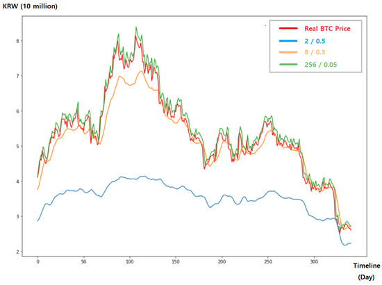
Figure 1.
Predicted values according to various hyperparameter settings.
In order to set the optimal hyperparameter values, it is necessary to find a combination of them that produces the minimum loss between actual values and predicted ones while substituting all the values as in the grid search method. It is, however, an ineffective and impractical method. Cost increases to determine the ideal combination are unavoidable as the number of hyperparameters to configure rises. Even with only three hyperparameters, an optimization with 10 criteria each requires 1000 experiments.
To solve this problem, some studies adopt a method that involves determining an optimal value for one of the hyperparameters first, then matching that value to one of the other parameters. Although this method reduces the time to find parameter values, there is a limitation that the best combination of values cannot be found, since it does not take into account all possible combinations of the parameter values. Using the above method, a study predicted future bitcoin price with two hyperparameters, the length of the input sequence and the number of hidden layer units [12]. They found an optimal value of the number of hidden layer units. With the found value, they determined the optimal input sequence length. They did not conduct experiments with every possible combination of the two parameters, so it was impossible to ensure that the values they found gave the best performance.
We conducted bitcoin price prediction experiments with this existing way. We assigned 4, 8, 12, 16, 20 LSTM units with seven time steps and found the optimal value that gave the best performance. With the optimal number of LSTM units, we ran experiments with 0.05, 0.1, 0.15, 0.2, 0.25 for the ratio of the dropout layer. Through these experiments, the existing method determined that (12, 0.05) was the optimal combination. Moreover, we ran experiments under every combination and found that (20, 0.1) performed the best. As shown in Figure 2, the best combination (20, 0.1) showed a minimum loss between the predicted bitcoin price and the actual ones. However, (12, 0.05) found by the existing approach showed quite different values from the actual value.
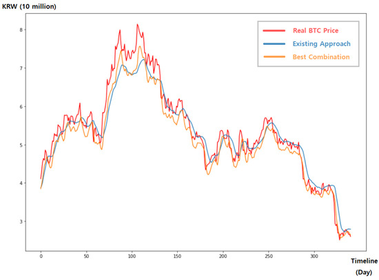
Figure 2.
Predicted values according to the hyperparameter optimization approach.
Some researchers utilize automatic hyperparameter optimization approaches, such as Bayesian optimization, but they also have a limitation that it is impossible to prove that the combination of values found by Bayesian optimization always shows the highest predictive performance [5].
In addition, even with the same hyperparameter configuration, the prediction performance varies according to the similarity between the data used for learning and future data. In dataset 1 of Figure 3, the learning data and the actual future data in the period where the model needs to be predicted are similar without significant changes. However, the learning data and the future one in dataset 2 are quite dissimilar. (Table 1 includes details about dataset 1 and dataset 2.) As shown in the figure, the two datasets use the same hyperparameter configuration and the same bitcoin price data, but show different prediction accuracies.
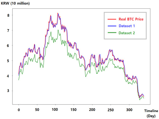
Figure 3.
Predicted values according to the similarities between training and future data under the same hyperparameter configuration.

Table 1.
Period and number of data collected.
For these reasons, we analyzed the predictive performance trends while adjusting three representative hyperparameters considering the similarity between the training data and future data. Based on our analysis, users can reduce the cost of optimizing hyperparameters without conducting experiments with every possible combination.
4. Experimental Environment
To demonstrate the direction of hyperparameter optimization for bitcoin price prediction, we conducted experiments with three hyperparameters: the number of time steps, the number of LSTM units, and the ratio of the dropout layer. By adjusting the hyperparameter values, we calculated the loss between the actual values and predicted ones. All experiments were conducted on a GPU provided by Google Colaboratory.
4.1. Data Collection and Normalization
In this paper, we collected closing daily price data from bitcoin price data from 28 October 2017 to 30 June 2022 using Open API provided by the Upbit exchange [13]. The collected data were classified according to the purpose: training data to learn the model, verification data to validate the model from the training process and test data to measure the actual predictive performance. In order to analyze the difference in prediction accuracy depending on the similarity between data used for learning and future data, we varied the data ranges used for learning with the same bitcoin price. As shown in Figure 4 and Table 1, dataset 1 was configured with a training period from 28 October 2017 to 3 February 2021 while the validation period was configured from 4 February 2021 to 24 July 2021. Dataset 2 had a shorter learning period from 28 October 2017 to 17 August 2020 than dataset 1. The data for training had low and stable values, whereas the data for validation and testing showed significantly higher and fluctuating values in dataset 1. In contrast to dataset 1, dataset 2 contained data that were similar to those used for training and verification, but the values for testing were very different from those used for learning.
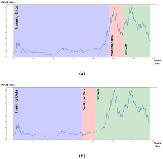
Figure 4.
Data classification for training, verification and test. (a) Dataset 1. (b) Dataset 2.
4.2. Model Design
We design a sequential LSTM model consisting of an LSTM layer, a dropout layer and a dense layer by using an LSTM neural network. We did not use an activation function in the output layer, because the input/output gate inside the LSTM cell contained sigmoid and tanh functions. We adopted Adam, which effectively mitigates severe local minima, as an optimizer and set the learning rate to 0.001, the most recommended default value. The mean squared error (MSE) was employed as a loss function and the batch size was 32. To avoid overfitting, we set the epoch size to 32 and used Keras’ EarlyStopping callback function to automatically terminate the training if the loss of verification data was not improved ten times.
4.3. Hyperparameter Configuration
As shown in Table 2, we classified the number of time steps into four and conducted experiments with 32 LSTM units and a dropout ratio of 10 for the dropout layer. The total number of combinations was 1280 and the flowchart in Figure 5 shows the experimental process. The experiments are conducted five times with these hyperparameter configurations, and average loss between actual values and predicted values are obtained.

Table 2.
Hyperparameter settings.
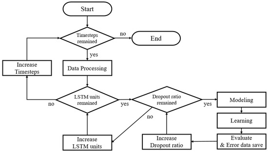
Figure 5.
Flowchart of the optimization experiment.
5. Predictive Performance Trends
To compare the predictive performance, we used the predictive loss by calculating the difference between the predicted values and the actual ones using the MSE. The losses are expressed on the z-axis with the number of LSTM units and the ratio of the dropout layer on the x-axis and y-axis at each time step value in Figure 6. We found several features for hyperparameter optimization through these visualized results.
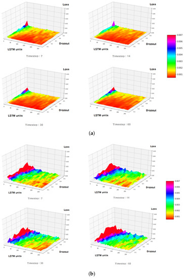
Figure 6.
Three-dimension planar graph of loss data according to time steps: (a) dataset 1 (70/10/20), (b) dataset 2 (50/10/40).
First, dataset 1 showed loss values that were lower than dataset 2. Although Figure 6a is mostly expressed in red with a loss of less than 0.001, Figure 6b hardly shows any red. The model created from dataset 1 was trained on stable data but was then verified on values that were rapidly changing. As a result, it was able to predict changes in the bitcoin price data used in the test stage. On the other hand, in dataset 2, it was difficult to predict a sudden price change in the test stage because the data used for training and verification had stable values. This suggests that if test data are significantly different from the data used for training and validation, a large prediction loss may occur.
Moreover, in both dataset 1 and dataset 2, the loss values decreased as the number of time steps increased until a certain point. After that, the loss values got worse as the number of time steps increased. Figure 6a shows that the dark red area, which indicate low loss values, is the widest at time step 30. However, the red area becomes smaller at time step 60. It is also difficult to find the red area at time step 60 in Figure 6b. Bitcoin prices are very sensitive to recent price variations. Thus, when large time steps are applied, the prediction performance is deteriorated as too-old data are included.
In all cases, regardless of the number of time steps and the number of LSTM units, we found that the loss was smaller when the ratio of the dropout layer was lower. Given the small quantity of bitcoin price data and the use of EarlyStopping in this paper, it was advantageous to always keep the ratio of the dropout layer low because overfitting had little impact on it.
In addition, it can be seen that under all time steps cases, the higher the number of LSTM units, the lower the loss values.
Dataset 1 showed no significant error changes between a small number of LSTM units and a large number of LSTM units, and generally showed low losses no matter the number of LSTM units. However, dataset 2 had a large difference in loss changes between a small number of LSTM units and a large number of LSTM units. This indicated that when the trend of the learning data and test data was similar, a good prediction performance could be quickly achieved even with a small number of LSTM units. However, it can be seen that a better prediction performance can be expected by increasing the number of LSTM units as much as possible in the case of considerable changes in trend between learning data and test data.
For the above reasons, the direction of hyperparameter optimization for bitcoin price prediction showing a high accuracy is as follows. In order to design a model with a high prediction performance, it is appropriate to select the number of time steps not too large and to set the lowest ratio of the dropout layer. Moreover, we considered the difference between future data and current data. Since the learning time grows as the number of LSTM units increases, it is recommended to keep the number of LSTM units low to reduce the cost of learning a model if data changes are not expected to be significant in the future. In contrast, if users expect data to fluctuate greatly, they must set a high number of LSTM units in order to make high-accuracy predictions.
6. Predictive Performance Evaluation
Based on the analysis, we performed experiments under five combinations of hyperparameters. According to the five predictive performance levels in Table 3, we evaluated the prediction performance by calculating the MSE and measured the learning time to make a prediction model. In addition, the predicted results are shown with the actual bitcoin price data in Figure 7 and Figure 8.

Table 3.
Representative combination of each level of performance.
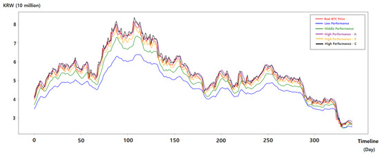
Figure 7.
Predicted values according to each hyperparameter combination.
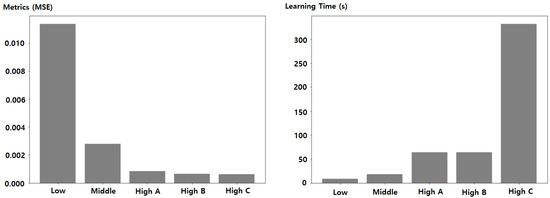
Figure 8.
MSE and learning time according to each hyperparameter combination.
As shown in the figures, the prediction performance corresponded to the direction of hyperparameter optimization analyzed. Because the prediction performance got better the larger the time step until a certain point, High A/B/C with a relatively large time step showed a higher performance than Low with 7 time steps and Middle with 14 time steps.
However, after 30 time steps, which is a certain point, it can be seen that the performance was rather reduced. High A had the same number of LSTM units and the same ratio of the dropout layer as High B. Figure 8 shows that High A had a higher MSE than High B.
Dataset 1 used in the experiment had a similar price trend between learning data and test data, so we could obtain a high predictive performance with only a low number of LSTM units. High B and High C had the same values of time steps and ratio of the dropout layer, but different numbers of LSTM units of 32 and 256. As can be seen in Figure 7, the predicted values of both High B and High C were quite close to the actual bitcoin price data and the difference in performance between them was not large. However, it can be seen in Table 3 and Figure 8 that High C took more than five times longer than High B to learn. Through this, it can be confirmed that if a severe difference between learning data and future data is not anticipated, users can save the cost of learning a model with a small number of LSTM units while obtaining a high prediction performance.
As for the ratio of the dropout layer, it can be seen that good predictive performance can be expected to be reduced as much as possible. Low and Middle, which had a relatively high ratio of the dropout layer of 0.5 and 0.4, had a lower predictive performance than High A/B/C which adopted 0.05 as the ratio for the dropout layer.
The price of bitcoin, which was used for this study, is representative of cryptocurrencies. Most cryptocurrencies are affected by the flow of the bitcoin price and have similar characteristics. As a result, our approach of hyperparameter optimization can be seamlessly applicable to predict other cryptocurrencies.
7. Related Work
There are many works utilizing machine learning in cryptocurrency data. One work analyzed the relationship between the price data of cryptocurrencies by using the correlation coefficient. Based on the analysis, the authors presented the cryptocurrencies suitable for a regression model [14]. Some researchers used news data to predict bitcoin price, because they considered that bitcoin price was affected by psychological factors [15,16]. Moreover, there was a study to predict the number of bitcoin transactions, in order to avoid the transaction delays which cause severe damage to the bitcoin market [17].
To provide a high predictive performance, existing cryptocurrency data prediction studies typically design a model using an RNN or LSTM neural network and they perform a hyperparameter optimization through experiments. To do this, some researchers conducted experiments with eight units in the hidden layer, one of hyperparameters [18]. In [17], the authors used two hyperparameters to obtain a high performance, but they did not consider every combination of the two parameters. They just picked the optimal value of the first parameter and then decided the optimal value of the second one based on the first one. In a similar way, ref. [18] specified the number of units of the hidden layer of an LSTM model as six and the sequence length as seven for their hyperparameter optimization. They found the optimal value of the number of hidden layers, then they performed experiments by adjusting the sequence length with the selected optimal number of hidden layers. Ref. [19] presented the key challenges to be solved in the hyperparameter optimization process and showed that studies were actively being conducted to develop various algorithms and software packages to solve them. In comparison to a grid search and manual search, ref. [20] assessed the effectiveness of hyperparameter optimization using random search. According to [21], automating grid and random searches enhance performance compared to manual searching. Additionally, ref. [22] provided a multiobjective hyperparameter optimization technique for CIFAR-10 and MNIST that used automated design space exploration (DSE) to reduce implementation costs while also enhancing performance. Ref. [23] summarized Bayesian optimization and recent studies using it for hyperparameter optimization, and ref. [24] conducted experiments using Bayesian optimization methods in the process of hyperparameter optimization of rock classification models and compared them to a grid search and a random search. In [25], the authors investigated the overhead for the expensive computational costs of the Bayesian method for hyperparameter optimization and proposed several scalable algorithms to relieve the overhead and accelerate the optimization.
8. Conclusions
By adjusting the tunable representative hyperparameters of the LSTM model, we analyzed the prediction performance trends in order to effectively determine the best configuration of hyperparameters for the bitcoin price. We utilized two datasets which had different ranges of data period for learning and testing. From the analysis, we found that a high prediction performance was obtained with a small ratio of the dropout layer regardless of the other two parameters. We found that the larger the time step value, the higher the prediction rate, but from a certain point onward, the performance deteriorated. When the data used for learning and future price were similar, a low number of LSTM units could achieve a high prediction, so with fewer LSTM units, we could get a high learning speed and a low learning cost. However, when the difference between learning data and future data was significant, a large number of LSTM units was required for a high performance. To find the optimal hyperparameters configuration efficiently with low cost, the users can take our results into consideration.
Future work: In this paper, we analyzed the direction of hyperparameter optimization by selecting three hyperparameters of LSTM. They were representative of hyperparameters, but we did not figure out the performance trend with the rest of parameters. Therefore, we plan to analyze the prediction performance with more hyperparameters in depth. We will also develop a guidance tool to automatically select values of each hyperparameter for a high predictive performance.
Author Contributions
Conceptualization, J.-H.K. and H.S.; methodology, J.-H.K. and H.S., software, J.-H.K.; validation, J.-H.K. and H.S.; investigation, J.-H.K.; writing-original draft preparation, J.-H.K.; writing-review and editing, H.S. All authors have read and agreed to the published version of the manuscript.
Funding
This research was funded by a 2021 Research Grant from Sangmyung University. (2021-A000-0389); corresponding author: Hanul Sung.
Data Availability Statement
Not applicable.
Conflicts of Interest
The authors declare no conflict of interest.
References
- Nakamoto, S. Bitcoin: A Peer-to-Peer Electronic Cash System. Available online: https://bitcoin.org/bitcoin.pdf (accessed on 20 November 2022).
- Binance. Available online: https://www.binance.com/en (accessed on 20 November 2022).
- Kim, S.W. Performance Analysis of Bitcoin Investment Strategy using Deep Learning. J. Korea Converg. Soc. 2021, 12, 249–258. [Google Scholar] [CrossRef]
- Won, J.G.; Hong, T.H. The Prediction of Cryptocurrency on Using Text Mining and Deep Learning Techniques: Comparison of Korean and USA Market. Knowl. Manag. Res. 2021, 22, 1–17. [Google Scholar] [CrossRef]
- McNally, S.; Roche, J.; Caton, S. Predicting the Price of Bitcoin Using Machine Learning; Institute of Electrical and Electronics Engineers Inc.: Piscataway, NJ, USA, 2018; pp. 339–343. [Google Scholar] [CrossRef]
- Joo, I.T.; Choi, S.H. Stock Prediction Model based on Bidirectional LSTM Recurrent Neural Network. J. Korea Inst. Inf. Electron. Commun. Technol. 2018, 11, 204–208. [Google Scholar] [CrossRef]
- Yu, Y.; Si, X.; Hu, C.; Zhang, J. A review of recurrent neural networks: Lstm cells and network architectures. Neural Comput. 2019, 31, 1235–1270. [Google Scholar] [CrossRef] [PubMed]
- Donkers, T.; Loepp, B.; Ziegler, J. Sequential User-Based Recurrent Neural Network Recommendations; Association for Computing Machinery, Inc.: New York, NY, USA, 2017; pp. 152–160. [Google Scholar] [CrossRef]
- Jeong, K.J.; Choi, J.S. Deep Recurrent Neural Network. Commun. Korean Inst. Inf. Sci. Eng. 2015, 33, 39–43. [Google Scholar]
- Srivastava, N.; Hinton, G.; Krizhevsky, A.; Salakhutdinov, R. Dropout: A Simple Way to Prevent Neural Networks from Overfitting. J. Mach. Learn. Res. 2014, 15, 1929–1958. [Google Scholar] [CrossRef]
- Yu, T.; Zhu, H. Hyper-Parameter Optimization: A Review of Algorithms and Applications. 2020. Available online: https://arxiv.org/abs/2003.05689 (accessed on 20 November 2022).
- Ji, S.H.; Baek, U.J.; Shin, M.G.; Goo, Y.H.; Yoon, S.H.; Kim, M.S. Design of LSTM Model for Prediction of Number of Bitcoin Transactions; Korean Network Operations and Management: Seoul, Republic of Korea, 2019; pp. 472–473. [Google Scholar]
- Upbit. Available online: https://upbit.com/ (accessed on 20 November 2022).
- Kwon, D.H.; Heo, J.S.; Kim, J.B.; Lim, H.K.; Han, Y.H. Correlation Analysis and Regression Test on Cryptocurrency Price Data; Korea Information Processing Society: Seoul, Republic of Korea, 2018; pp. 346–349. [Google Scholar] [CrossRef]
- Kim, E.M.; Hong, J.W. The Prediction Model of Cryptocurrency Price Using News Sentiment Analysis and Deep Learning; Korea Society of IT Services: Seoul, Republic of Korea, 2020. [Google Scholar]
- Gang, M.G.; Kim, B.S.; Shin, H.J. Machine Learning based Prediction of Bitcoin Price Fluctuation Using News Data; Korean Network Operations and Management: Seoul, Republic of Korea, 2021; pp. 38–39. [Google Scholar]
- Ji, S.H.; Baek, E.J.; Shin, M.G.; Park, J.S.; Kim, M.S. A Study on the Prediction of Number of Bitcoin Network Transactions Based on Machine Learning. KNOM Rev. 2019, 22, 68–76. [Google Scholar]
- Gang, M.G.; Kim, B.S.; Shin, M.G.; Baek, U.J.; Kim, M.S. LSTM-Based Prediction of Bitcoin Price Fluctuation using Sentiment Analysis; Korean Institute of Communications and Information Sciences: Seoul, Republic of Korea, 2020; pp. 561–562. [Google Scholar]
- Claesen, M.; Moor, B.D. Hyperparameter Search in Machine Learning. 2015. Available online: https://arxiv.org/abs/1502.02127 (accessed on 20 November 2022).
- Bergstra, J.; Bengio, Y. Random Search for Hyper-Parameter Optimization. J. Mach. Learn. Res. 2012, 13, 281–305. [Google Scholar]
- Zahedi, L.; Mohammadi, F.G.; Rezapour, S.; Ohland, M.W.; Amini, M.H. Search Algorithms for Automated Hyper-Parameter Tuning. arXiv 2021, arXiv:2104.14677. [Google Scholar]
- Smithson, S.C.; Yang, G.; Gross, W.J.; Meyer, B.H. Neural Networks Designing Neural Networks: Multi-Objective Hyper-Parameter Optimization; Institute of Electrical and Electronics Engineers Inc.: Piscataway, NJ, USA, 7–10 November 2016. [Google Scholar] [CrossRef]
- Nguyen, V. Bayesian Optimization for Accelerating Hyper-Parameter Tuning; Institute of Electrical and Electronics Engineers Inc.: Piscataway, NJ, USA, 2019; pp. 302–305. [Google Scholar] [CrossRef]
- Choi, Y.U.; Yoon, D.U.; Choi, J.H.; Byun, J.M. Hyperparameter Search for Facies Classification with Bayesian Optimization. Geophys. Geophys. Explor. 2020, 23, 157–167. [Google Scholar] [CrossRef]
- Sui, G.; Yu, Y. Bayesian Contextual Bandits for Hyper Parameter Optimization. IEEE Access 2020, 8, 42971–42979. [Google Scholar] [CrossRef]
Publisher’s Note: MDPI stays neutral with regard to jurisdictional claims in published maps and institutional affiliations. |
© 2022 by the authors. Licensee MDPI, Basel, Switzerland. This article is an open access article distributed under the terms and conditions of the Creative Commons Attribution (CC BY) license (https://creativecommons.org/licenses/by/4.0/).