A New Approach to Calibrating Functional Complexity Weight in Software Development Effort Estimation

Abstract

Function point analysis is a widely used metric in the software industry for development effort estimation. It was proposed in the 1970s, and then standardized by the International Function Point Users Group, as accepted by many organizations worldwide. While the software industry has grown rapidly, the weight values specified for the standard function point counting have remained the same since its inception. Another problem is that software development in different industry sectors is peculiar, but basic rules apply to all. These raise important questions about the validity of weight values in practical applications. In this study, we propose an algorithm for calibrating the standardized functional complexity weights, aiming to estimate a more accurate software size that fits specific software applications, reflects software industry trends, and improves the effort estimation of software projects. The results show that the proposed algorithms improve effort estimation accuracy against the baseline method.

1. Introduction

Software estimation has long been considered a core issue that directly affects success or failure. According to the Standish Group [1], the failure rate of a part of a project or of a whole project is likely to be up to 83.9% (as of 2019). One of the reasons for this failure is inaccurate cost and effort estimates. In fact, to obtain software projects, companies participating in tenders must submit bids that include cost, manpower, and software development time. To be able to win the tender, the companies participating need to give a reasonable estimate of the cost, manpower, and time required to carry out the project. Reasonability here does not mean underestimating the price, because in so doing the company will not gain (if not lose) when completing the project. It is also not reasonable to overestimate the price, because then it is certain that the company will not win the bid. Therefore, a project estimate is considered reasonable only if it accurately reflects the project’s actual value.

Throughout the software development process, no matter what software management model a company uses, project leaders often have to plan the work for software development milestones, plan the next milestone, and recalculate the work done in the previous milestone. All of these tasks require software estimation skills. Many methods have previously been proposed to solve the software estimation problem. Due to the increasing demand for more efficient and accurate estimation methods that can work with more complex software projects, such estimation methods need to be refined. Software estimation methods can be classified into three main groups: non-algorithmic, algorithmic, and machine learning approaches [2,3]. In the non-algorithmic category, there are two representative methods: expert judgement (EJ) [4] and analogy [5]; with these methods, experts play the most significant role in judgement. Of course, previous samples (historical dataset) also play another important role. In the algorithmic category, an algorithm takes the first role. software lifecycle management (SLIM) [6], the Constructive Cost Model (COCOMO) [7], and function point analysis (FPA) and the International Function Point User Group (IFPUG FPA) [8,9] are representative models. The IFPUG FPA method arose as an alternative to other solutions. Other methods based on IFPUG FPA —such as COSMIC [10], FiSMA [11], MarkII [12], and NESMA [13]—were proposed to improve some aspects of the original method. In the last category, machine learning techniques have been used in recent years to supplement or replace the other two techniques. Most software cost estimation techniques use statistical methods, which cannot provide strong rationales and results. Machine learning approaches may be appropriate in this area because they can increase the accuracy of estimates by training the estimation rules and repeating the running cycles. Examples include fuzzy logic modelling, regression trees, artificial neural networks (ANNs), and case-based reasoning (CBR). These methods have explored the applicability of machine learning techniques to software effort estimation; they have objective and analytical formulas that are not limited to a specific number of factors. However, most methods only evaluate the limitations of modelling techniques on a particular dataset, reducing the generalisability of the observed results. Some researchers also overlook statistical testing of the results obtained or evaluation of the models against the same dataset used to generate the models [14].

This paper is organised as follows: Section 1 is the introduction. The problem formulation and the contributions are described in Section 2. Section 3 illustrates the related works. Section 4 presents the background, with a brief overview of the FPA method, Bayesian ridge regression model, and voting regressor model. The proposed research methodology is expressed in Section 5, in which we introduce the dataset and data processing, experimental setup, and evaluation criteria. Section 6 presents the experimental results and discussion. Section 7 describes the threats to validity. We finalise our paper in Section 8 with the conclusion.

2. Problem Formulation

FPA has been used for over four decades, and has proven to be a dependable and consistent method [15] of sizing software for project estimation and productivity or efficiency comparisons. Although it has made significant contributions in the software industry, it still has many problems. In an earlier systematic literature review [16], we mentioned some limitations of FPA. The inadequacy of complexity weight is still a major problem. In addition, the locality of the dataset that builds the FPA approach (IBM projects) does not reflect the entire global software industry. Many previous studies have suggested a new functional complexity weight [17,18] in different ways. In [18], Xia et al. proposed a new functional complexity table based on an IFPUG FPA calibration model called Neuro-Fuzzy Function Point Calibration Model (NFFPCM), which integrates the power of neural networks and fuzzy logic. Nevertheless, the method needs to be changed in line with changes in the modern software industry.

Another issue that needs to be mentioned is the specificity of each piece of software. Differences in the purpose of the software being developed lead to different approaches. With FPA, a method that applies to all software estimation cases needs to be revisited; this was the motivation for us to propose a new, up-to-date, nonlocal functional complexity weight that reflects the software industry.

After counting the function points (FPs), we can calculate the effort and then write a report [9] based on these FPs. At this point, the FPA counting process is considered complete. However, one question is whether we can further improve the effort after the calculation of the counting process. Recent studies [19,20,21,22,23] show that combining an ensemble model and other approaches provides better results than using a single model. This study applies an ensemble model to the result after the counting and calculating effort to improve the accuracy gained from FP counting based on the proposed functional complexity weight.

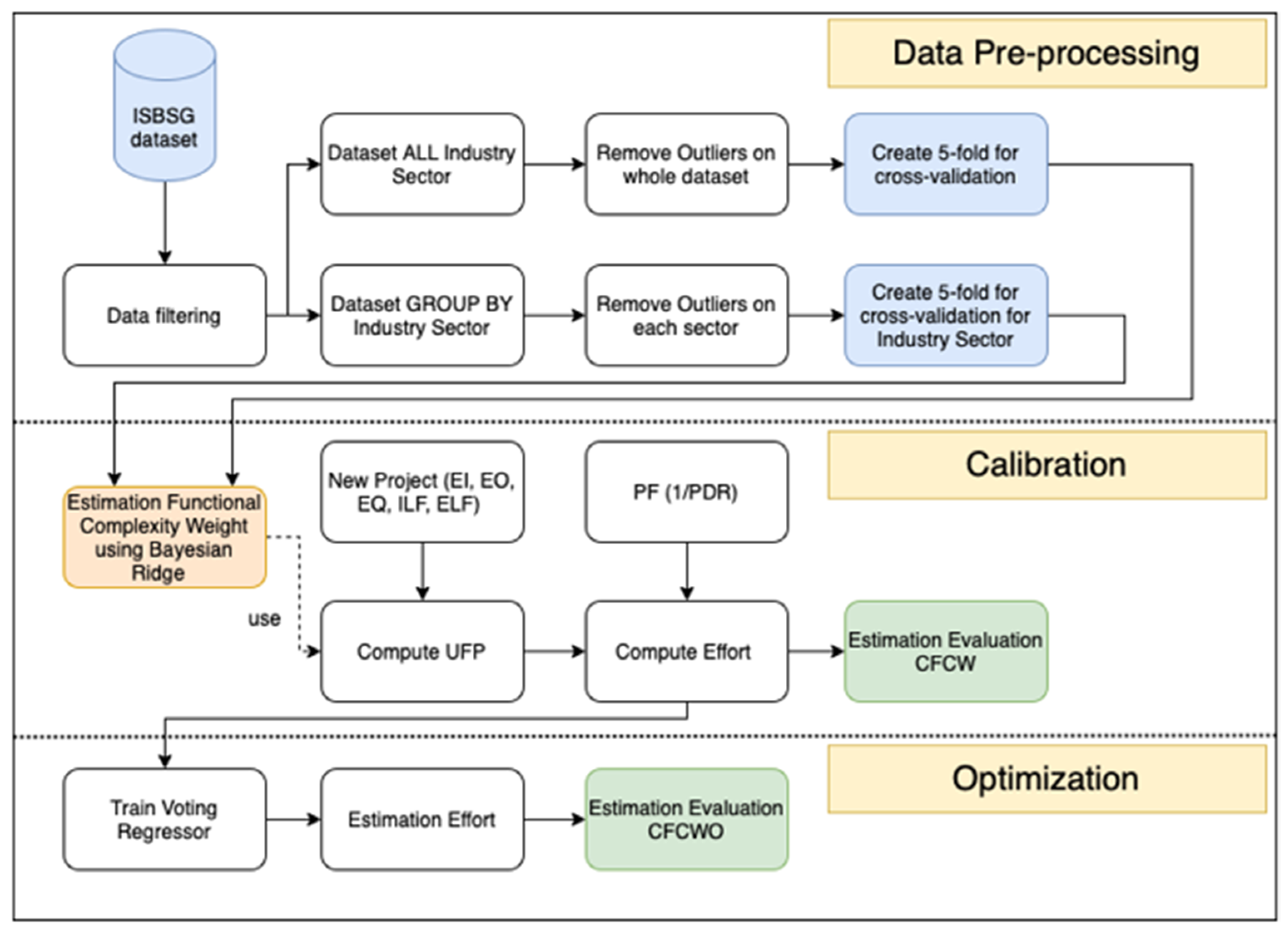
This study aims to propose an algorithm called the calibration of functional complexity weight (CFCW) algorithm. The proposed algorithm is based on the FPA method combined with regression methods implemented in the International Software Benchmarking Standards Group (ISBSG) dataset Release 2020 R1 [24].

Many companies around the world contribute to the ISBSG dataset, so the locality problem can be solved. In addition, the 2020 database update addresses the out-of-date issue. Many recent studies (for example, [25,26,27]) used the industry sector (IS) as a categorical variable for dataset segmenting in their research. Our study tested a second approach—the calibration of functional complexity weight with optimisation based on an ensemble model called the voting regressor (CFCWO).

Based on the above issues, we propose three research questions:

RQ1:

Is the accuracy of the proposed CFCW algorithm better than that of the IFPUG FPA or NFFPCM methods?

RQ2:

Does the advanced CFCWO algorithm outperform the CFCW algorithm?

RQ3:

How accurate is the estimation for each sector compared to an ungrouped dataset?

To answer these research questions, we conducted an experimental study to evaluate the estimation accuracy of the proposed approaches.

Contributions

The main contributions of this research are as follows:

• In the first phase, a new CFCW algorithm for the calibration of functional complexity weight is proposed;
• In the second phase, the result from the first phase is optimised by using a voting regressor to estimate the final software effort—the CFCWO algorithm is proposed;
• The IFPUG FPA method is compared to the CFCW algorithm for ungrouped data and data grouped by IS;
• The CFCW algorithm is compared to the CFCWO algorithm for ungrouped data and data grouped by IS.

3. Related Work

FPA is a standardised method for determining the size of software based on its functional requirements; it is designed to be applicable regardless of programming language or implementation technology. Albrecht [8] recommends FPA to measure the size of a system that processes data from end-users. Since its introduction, much research has been carried out to improve its accuracy.

Al-Hajri et al. [17] introduced a modification weighting system for measuring FP using an ANN model (backpropagation technique). In their study, a weighting system was built based on four steps: (1) using the original weighting system as a baseline to establish new weights; (2) using the DETs/RETs of the original system’s FPA to calculate the new values, training these new values with an ANN, and then predicting the values of the new weights; (3) applying the new weights and the original weights in the FPA model; and (4) calculating the size of FPs as a function of the original weights and the new weights. Wei et al. [28] proposed a different sizing approach by integrating the new calibrated FP weight proposed in [18] into a complexity assessment system for object-oriented development effort estimation. Misra et al. [29] proposed a metrics suite that helps in determining the complexity of object-oriented projects by evaluation of message complexity, attribute complexity, weighted class complexity, and code complexity.

Dewi et al. [30] produced a formula for estimating the cost of software development projects, especially in the field of public service applications; the authors modified the complexity adjustment factor to 16 instead of the 14 used in the standard FPA method and; as a result, the accuracy was improved by 7.19%.

In the study of Leal et al. [31], the authors investigated the use of nearest-neighbours linear regression methods for estimation in software engineering. These methods were compared with multilayer perceptron neural networks, radial basis function neural networks, support-vector regression, and bagging predictors. The dataset used in the study was a NASA software project. Based on the relative error and the estimation rate, the nearest-neighbours linear regression methods outperformed the others.

In a survey of applying ANNs to software estimation, Hamza et al. [32] provided an overview of the use of ANN methods to estimate development effort for software development projects; the authors offered four main ANN models, including (1) feedforward neural networks; (2) recurrent neural networks; (3) radial basis function networks; and (4) neuro-fuzzy networks. The survey also explains why those methods are used and how accurate they are.

In the endeavour of estimating the effort needed for the next phase or the remaining effort needed to finish a project, Lenarduzzi et al. [33] conducted an empirical study on the estimation of software development effort. The estimation was broken down by phase so that estimation could be used throughout the software development lifecycle. This means that the effort needed for the next phase at any given point in the software development lifecycle is estimated. Additionally, they estimated the effort required for the remaining part of a software development process. The ISBSG dataset was used in the study. The results show statistically significant correlations between effort expended in one period and effort expended in the following period, effort expended in one period and total effort expended, and accumulated effort up to the present stage and remaining effort. The results also indicate that these estimation models have different degrees of goodness of fit. Further attributes, such as the functional size, do not significantly improve estimation quality.

In [25,34], the authors presented an influence analysis of selected factors (FP count approach, business area, IS, and relative size) on the estimation of the work effort for which the FPA method is primarily used. They also studied the factors that influence productivity and the productivity estimation capability in the FPA method. Based on these selected factors and experimentally, the authors proved that the selected factors have specific effects on work effort estimation accuracy.

In [35], from software features, the authors used various machine learning algorithms to build a software effort estimation model. ANNs, support-vector machines, K-star, and linear regression machine learning algorithms were appraised on a PROMISE dataset (called Usp05-tf) with actual software efforts. The results revealed that the machine learning approach could be applied to predict software effort. In the study, the results from the support-vector machines were the best.

In [36], the authors conducted a comparison between soft computing and statistical regression techniques in terms of a software development estimation regression problem. Support-vector regression and ANNs were used as soft computing methodologies, and stepwise multiple linear regression and log-linear regression were used as statistical regression methods. Experiments were performed using the NASA93 dataset from the PROMISE software repository, with multiple dataset pre-processing steps performed. The authors relied on the holdout technique associated with 25 random repetitions with confidence interval calculation within a 95% statistical confidence level. The 30 pre-evaluation criteria were used to compare the results. The results of the study show that the support-vector regression model has a significant impact on precision.

4. Background

4.1. IFPUG FPA

Albrecht [8] first introduced FPA in 1979, and presented the FP metric to measure the functionality of a project. This was proposed in response to a number of problems with other system size measures, such as lines of code. In 1986, the International Function Point User Group (IFPUG) [37] promoted and popularised effective software development and maintenance management through FPA.

The IFPUG is currently the governing body for FPA, and is responsible for improving and developing counting rules and other related matters. Since the IFPUG was created, the original FPA method has been known as the IFPUG’s FPA. In this study, the standard FPA method concept refers to the IFPUG FPA method. FPA is currently standardised by ISO/IEC 20926:2010 [38]; this standard specifies a set of definitions, rules, and steps for application [9]. There are six phases in counting standards; in this study, we are only interested in two phases: (1) data function and transactional function measurement, and (2) functional size measurement.

The first-phase results are the unadjusted function points (UFPs) and the value adjustment factor (VAF) values. The UFP value can be determined based on estimations of the number of transactional functions (external input (EI), external output (EO), or external inquiry (EQ)) and data functions (internal logic files (ILFs), and external interface files (EIFs)). These components are called base functional components. Each of these, in turn, is judged as low (L), average (A), or high (H), and assigned a weight accordingly.

Table 1. Data and transactional function complexity.

		Component
		EI	EO	EQ	EIF	ILF
Complexity weight	Low	3	4	3	5	7
	Average	4	5	4	7	10
	High	6	7	6	10	15

shows the available complexity weight of the components.

The UFP total sets the number of types in groups, multiplies them by complexity weights, and finds the sum of all fields, as in Equation (1):

$$UFP={\displaystyle \sum }_{i=1}^n{\displaystyle \sum }_{j=1}^m(S_{ij}\times W_{ij})$$

(1)

where $S_{ij}$ represents the total of each functional component, $W_{ij}$ represents the complexity weights, n is the number of types, and m is the number of complexity groups.

The VAF count is based on the rate of 14 general system characteristics (GSCs): data communications, distributed data processing, performance, heavily used configuration, transaction rate, online data entry, end user efficiency, online update, complex processing, reusability, installation ease, operational ease, multiple sites, and facilitate change.

There are six influence levels of GSC criteria, with the system being determined as a value from 0 to 5 contingent on the level: 0—no influence; 1—incidental influence; 2—moderate influence; 3—average influence; 4—significant influence; and 5—strong influence throughout. The VAF count is adjusted as follows:

$$VAF=0.65+0.01\times {\displaystyle \sum }_{i=1}^{14}\left(F_i\times rating\right)$$

(2)

The second-phase result is the adjusted function points (AFPs) value, which can be obtained using Equation (3):

$$AFP=UFP\times VAF$$

(3)

To estimate the effort after AFP counting, we should use another parameter. The productivity factor (PF) was described as the relationship between one FP and the number of hours needed for its development by one person. Productivity and PF were studied in [39,40]. The following formula can be used to calculate the effort using the PF:

$$Effort=AFP\times PF$$

(4)

ISBSG uses the productivity delivery rate (PDR) as a metric for efficiency. The PDR is measured in person-hours per FP. From the PDR, we can derive the PF in FPs per person-hour. We can see that the PDR is the inverted value of the PF (and vice versa) [9].

In our study, the IFPUG FPA method is the base method for proposing the new model; it is also used for the base compared with the proposed model. Additionally, the terms FPA and IFPUG FPA have the same meaning, and are interchangeable.

4.2. Bayesian Ridge Regression Model

The full Bayesian regression inference uses the Markov chain Monte Carlo algorithm to construct models [41]. The Bayesian modelling framework has been reputed for its ability to deal with a hierarchical data structure. In Bayesian regression techniques, regularisation parameters can be included in the estimation procedure. A regularisation parameter is not hard set, but is tuned to the data at hand. This can be done by introducing non-informative priors over the hyperparameters of the model. The $l_2$ regularisation used in ridge regression and classification is equivalent to finding a maximum a posteriori estimate under a Gaussian prior over the coefficients with precision. Instead of setting the lambda manually, this variable can be randomly estimated from the available data [42]. To acquire a fully probabilistic model, the output y is assumed to be Gaussian distributed around $X\omega$:

$$p\left(y|X,\omega ,\alpha \right)=\aleph \left(y|X\omega ,\alpha \right)$$

(5)

where $\alpha$ is treated as a random variable that is to be estimated from the data.

Bayesian ridge regression (BRR) is a probabilistic method that builds a regression model using Bayesian inference; it combines prior information about parameters (the coefficient of software features) with the observed training data in order to acquire the parameters’ posterior distribution [42]. The prior for the coefficient $\omega$ is specified by a spherical Gaussian:

$$p\left(\omega |\lambda \right)=\aleph \left(\omega |0,{\lambda }^{-1}{I}_p\right)$$

(6)

The priors over $\alpha$ and $\lambda$ are picked to be gamma distributions [43]—the conjugate prior for the precision of the Gaussian distribution.

In our study, the BRR plays a significant role in the calibration phase (see Figure 1).

4.3. Voting Regressor Model

The ensemble is a learning method that uses a specific aggregation mechanism to create a collection of prediction models, and then uses a weighted vote of their initial results to obtain the final solution [44,45,46,47,48]. The principal premise is that if techniques work together as a committee with reliable methods, they may be improved and generate more significant results [44]. As a result, this method is excellent for predicting software effort, since each model has its assumptions and setup parameters, allowing the ensemble to perform exceptionally well with some desirable statistical qualities [45]. Idri et al. [22,23] conducted a systematic literature review and mapping study, and discovered that (1) ensemble effort estimation techniques are more accurate than solo methods, (2) homogeneous ensembles are the most investigated, (3) machine learning techniques are the most used solo techniques to construct ensembles, and (4) there are two types of combiner rules used to estimate ensemble effort estimation: linear and nonlinear.

A voting regressor [46] is based on the idea of integrating various machine learning approaches to return uniform average projected values. A voting regressor is a technique that fits each of the base regressors to the entire dataset. A regressor such as this can help a group of estimators with similar performance levels to balance out their individual flaws. When the predictors are as independent as possible, ensemble approaches perform best. In general, each regressor is trained using a distinct technique, in order to make each prediction more independent of the others. This increases the likelihood that they will make a variety of blunders, which will improve the ensemble’s performance. A voting regressor can be applied for classification or regression. Each label’s predictions are combined with regard to classification, and the label with the most votes is chosen. In the case of regression, this entails computing the mean of the predictions from the models. According to Witten et al. [47], a voting ensemble is appropriate when all applicable models should perform well on a predictive modelling task; in other words, the models used in the ensemble must mostly agree.

In our study, the voting regressor was used in the CFCWO algorithm in the optimization phase (Figure 1).

5. Research Methodology

In this section, we present the research methodology. This includes describing the data to be used, along with the data processing and the experimental setup. In addition, evaluation criteria are introduced here.

5.1. Experimental Setup

In this section, we describe the experimental process, which is graphically illustrated in Figure 1.

In the data pre-processing phase (Figure 1), data filtering and cleaning were performed to create the working dataset (see following section). This dataset was used for two branches of experiments: experiments on ungrouped data (all sectors), and experiments on grouped data, where IS categorical variables were used for grouping. The fivefold cross-validation was used to create a training/testing fold. The dataset we used in our experiments was the ISBSG repository August 2020 R1 [24]. In our study, the criteria for data filtering were as follows:

• We selected records with the IFPUG counting approach (including IFPUG Old and IFPUG 4+);
• Only the records where the data quality rating is A or B has been selected;
• The development type was new development;
• The rows with an empty value of base functional components were eliminated;
• Rows with empty values in the industry sector column were removed;
• The rows with empty values in normalised productivity delivery rate and summary work effort (SWE) were also erased;
• We filled the VAF blank cells with the values obtained from Equation (3).

According to Lichtenberg and Şimşek [49], the number of records in a dataset is large enough to be eligible for a given training set to attain the most satisfactory results. M. Hammad [35] also proved that some algorithms learn perfectly as the size of the training set increases. In our case, after many tests and evaluations, the results from ISs with over 30 records gave the best results. For the ISs that did not satisfy this condition (the number of records is less than 30), we gathered them into a group named “Others”. Figure 2 shows a histogram of the dataset after being processed.

We notice that there is a possibility that the data may be noisy because some SWE values are too far from the mean group. In this study, we used the interquartile range (IQR) method [50,51] on these features to determine and remove outliers, with the lower boundary being 0.15 and the upper boundary being 0.85. Figure 3 and Figure 4 show the description of the dataset before and after the removal of outliers, respectively.

The calibration phase (Figure 1) represents the CFCW algorithm. The CFCW works as follows:

• Bayesian ridge regression (Section 4.2) is employed;
• CFCW elicits the complexity weights for the EI, EO, EQ, EIF, and ELF variables using Bayesian ridge regression;
• The UFP is calculated by using a newly estimated complexity weight for each of the variables (EI, EO, EQ, EIF, and ELF);
• Estimated effort is obtained by multiplying UFP by the VAF and, finally, by multiplying by PF.

The optimisation phase (Figure 1) represents the CFCWO algorithm, which works as follows:

• Effort from CFCW (calibration phase) is used as input;
• The voting regressor (Section 4.3) algorithm is employed;
• Voting regressor is an ensemble model, consisting of four estimators (

  Table 2. Base estimators of the voting ensemble model.

  Algorithm	Implementation	Parameters
  Random forests	sklearn.ensemble.RandomForestRegressor	n_estimators = 200, random_state = 0
  Bayesian ridge	sklearn.linear_model. BayesianRidge	n_iter = 300
  ANN	sklearn.neural_network. MLPRegressor	tol = 0.00001, max_iter=10000, momentum = 0.000001
  Lasso	sklearn.linear_model. Lasso	alpha = 0.01, selection = ‘random’, random_state = 63

  );
• CFCWO optimises estimated effort by CFCW by minimising the error to SWE (know effort from dataset).

Tested Models

The CFCW model and CFCWO model were tested on datasets with and without IS filtering. The variant called “all sectors” used the whole dataset without IS grouping. The IS was used as a grouping variable, allowing us to test both models on each IS independently (as seen in the Results section). The following is a brief description of the compared models:

• CFCW—effort is computed using the IFPUG approach; complexity weights are estimated by Bayesian ridge regression; PF (PDR) is the mean from all ISs or based on each IS;
• CFCWO—effort is estimated using a trained voting regressor, where the regressor is the effort value from CFCW, and the dependent variable is the SWE value (from the dataset); again, variant for all sectors and per sector were tested.

We performed a process using the voting ensemble model with four base estimators in the estimation effort optimization. These estimators and their parameters are described in Table 2.

CFCWW and CFCWO were compared to the following models:

• IFPUG FPA [37]—effort is computed using the IFPUG approach; IFPUG-based complexity weights and PF (PDR) from the dataset (mean from all sectors or based on each sector);
• NFFPCM [18]—effort is computed using IFPUG approach; complexity weight from the study of Xia et al. and PF (PDR) from the dataset (mean from all sectors or based on each sector).

5.2. Evaluation Criteria

Regarding measurement accuracy, according to Foss et al. [52], there have been many investigations and evaluations of the suitability of error functions proposed and used thus far. However, there is no universal solution to the problem of choosing good predictive models from among several alternatives; this means that each accuracy indicator has certain advantages over the others. Kitchenham et al. [53] pointed out that the crucial factor for meaningful comparisons between predictive models is identifying what each error function uses for actual measurements. This study uses the most common and widely used measures to evaluate the predictability of comparative models and the accuracy of the proposed model.

MAE (mean absolute error) [54]:

$$MAE=\frac{1}{N}{\displaystyle \sum }_{i=0}^N\left|y_i-{\widehat{y}}_i\right|$$

(7)

MSE (mean squared error) [55]:

$$\begin{array}{c}MSE=\frac{1}{N}\end{array}{\displaystyle \sum }_{i=1}^N{(y_i-{\widehat{y}}_i)}^2$$

(8)

RMSE (root-mean-square error) [56]:

$$RMSE=\sqrt{\frac{1}{N}{\displaystyle \sum }_{i=1}^N{\left(y_i-{\widehat{y}}_i\right)}^2}$$

(9)

MAPE (mean absolute percentage error) [57]:

$$MAPE=\frac{1}{N}{\displaystyle \sum }_{i=0}^N\left|\frac{y_i-{\widehat{y}}_i}{y_i}\right|\ast 100$$

(10)

where $y_i$ is the actual value, ${\widehat{y}}_i$ is the predicted value, and N is the number of projects.

6. Results and Discussion

In this section, we evaluate the accuracy of the proposed CFCW and CFCWO from the experimental results. We compare the IFPUG FPA and NFFPCM models to CFCW and CFCWO algorithms. All experiments for all sectors and for data grouped by IS were calculated.

The calibrated functional complexity weight values obtained from the experiment are listed in

Table 3. Calibrated functional complexity weight.

		IFPUG FPA	All Sectors	Banking	Communication	Financial	Government	Insurance	Manufacturing	Service Industry	Others
EI	Low	3	3.48	1.73	1.10	3.52	0.41	2.09	3.49	3.95	3.17
	Average	4	1.17	1.21	3.97	3.98	7.76	4.18	0.99	5.50	1.33
	High	6	8.35	7.90	3.86	4.64	7.04	4.15	8.54	6.72	9.55
EO	Low	4	3.49	3.06	3.45	4.9	2.47	3.78	3.58	3.83	3.03
	Average	5	4.42	5.37	2.54	2.01	5.59	4.78	5.28	4.74	4.20
	High	7	4.94	8.09	7.48	7.06	6.09	4.80	6.89	6.37	7.20
EQ	Low	3	3.79	0.71	1.87	3.35	2.98	3.94	2.00	2.42	2.81
	Average	4	5.94	4.39	3.38	3.82	4.38	5.70	4.81	4.26	6.31
	High	6	2.28	9.48	4.22	5.86	2.57	6.42	5.78	4.81	3.34
ILF	Low	5	5.13	6.26	4.77	4.28	8.22	4.96	5.52	3.07	3.20
	Average	7	7.22	2.24	10.60	8.92	5.31	4.14	7.99	3.53	9.93
	High	10	9.58	15.96	9.72	8.22	7.24	10.72	6.38	5.82	11.44
EIF	Low	7	7.13	2.23	7.22	8.97	6.20	11.54	8.55	5.82	6.61
	Average	10	7.04	10.16	9.72	12.46	12.84	2.48	1.88	17.32	4.40
	High	15	15.75	24.9	7.68	9.48	18.33	9.24	22.41	16.59	12.90

. According to the values of the individual parameters EI, EI, EQ, ELF, and ILF, the calibrated values of the scales differ from the original values. The minimum percentage deviation is approximately 2% on an ungrouped dataset, while the maximum deviation is nearly 242% against standard weights. The individual ISs show an even greater variance in deviations.

Figure 5 shows a comparison of efforts estimated by the IFPUG FPA, NFFPCM, CFCW, and CFCWO methods versus the real SWE. The effort estimated by the CFCWO approach was closest to the SWE (in all cases). This means that the proposed CFCWO approach also outperforms the IFPUG FPA, NFFPCM, and CFCW methods.

Table 4. MAE evaluation results and improvement percentages.

		MAE			Improvement of CFCW vs. IFPUG FPA (%)	Improvement of CFCW vs. NFFPCM (%)	Improvement of CFCWO vs. CFCW (%)
	IFPUG FPA	NFFPCM	CFCW	CFCWO
All Sectors	678.72	758.42	641.68	565.37	5.46	15.39	11.89
Banking	463.96	493.09	301.02	244.76	35.12	38.95	18.69
Communication	422.76	322.31	204.82	191.73	51.55	36.45	6.39
Financial	210.16	569.07	169.11	131.60	19.53	70.28	22.18
Government	513.30	1012.22	480.05	450.62	6.48	52.57	6.13
Insurance	417.08	422.45	325.86	305.46	21.87	22.86	6.26
Manufacturing	207.29	398.12	192.84	167.97	6.97	51.56	12.90
Service Industry	319.78	1051.87	294.48	257.72	7.91	72.00	12.48
Others	344.90	619.79	278.00	247.53	19.40	55.15	10.96
Mean (Sectors)	362.40	611.12	280.77	249.67	22.52	49.98	11.08

shows the MAE value when using the IFPUG FPA, NFFPCM, CFCW, and CFCWO algorithms, along with the percentage improvement value of the CFCW method compared to the IFPUG FPA method, and the percentage improvement value of the CFCWO algorithm compared to the CFCW algorithm. Accordingly, the lowest improvement value of the CFCW method compared to the IFPUG FPA method was in the government sector, with 6.48%, while the highest was in the communication sector, with 51.55%. Overall, the estimated effort by the CFCW algorithm improved by 5.46%, while that by the CFCWO algorithm was enhanced by 11.89%.

According to this MAE evaluation criterion, the NFFPCM does outperform IFPUG FPA in most sectors, except for communication. The CFCW results are always better than that of NFFPCM, and the CFCWO is the same.

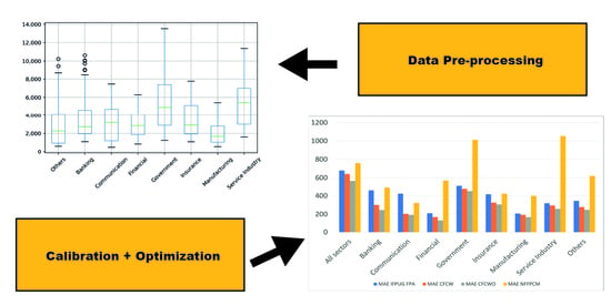
Figure 6 shows a comparison of the results from a visual perspective. The MAE of the CFCWO algorithm is always the smallest, indicating the best estimation accuracy.

Table 5. MAE percentage difference of the individual sectors compared to the ungrouped dataset.

	IFPUG FPA (%)	NFFPCM (%)	CFCW (%)	CFCWO (%)
Banking	31.64	34.98	53.09	56.71
Communication	37.71	57.50	68.08	66.09
Financial	69.04	24.97	73.65	76.72
Government	24.37	−33.46	25.19	20.3
Insurance	38.55	44.30	49.22	45.97
Manufacturing	69.46	47.51	69.95	70.29
Service Industry	52.89	−38.69	54.11	54.42
Others	49.18	18.28	56.68	56.22
Mean	46.61	19.42	56.25	55.84

shows the percentage difference based on the MAE evaluation criteria for each IS compared to the same algorithm applied to all sectors.

Table 6. MAPE evaluation results and improvement percentages.

		MAPE			Improvement of CFCW vs. IFPUG FPA (%)	Improvement of CFCW vs. NFFPCM (%)	Impprovement of CFCWO vs. CFCW (%)
	IFPUG FPA	NFFPCM	CFCW	CFCWO
All Sectors	14.18	19.01	13.61	12.72	4.01	28.41	6.56
Banking	10.63	13.43	7.36	6.28	30.76	45.20	14.67
Communication	13.99	13.81	10.09	8.22	27.94	26.94	18.53
Financial	9.08	24.48	7.91	7.15	12.89	67.69	9.61
Government	7.40	19.21	7.32	7.02	1.08	61.89	4.10
Insurance	11.17	12.75	9.52	8.99	14.77	25.33	5.57
Manufacturing	11.19	19.73	10.42	9.59	6.88	47.19	7.97
Service Industry	7.41	16.93	6.64	5.94	10.39	60.78	10.54
Others	9.57	18.94	8.10	7.71	15.36	57.23	4.81
Mean (Sectors)	10.06	17.41	8.42	7.61	16.26	49.03	9.59

shows the MAPE evaluation values of the proposed approach and the improvement of the CFCW and CFCWO methods compared to the IFPUG FPA method. Each value in the CFCW column is always smaller than that in the FPA column, and each value in the CFCWO column is smaller than that in the CFCW column. This means that the CFCW method is better than the FPA method, and the CFCWO algorithm is better than the CFCW algorithm. The superiority of the CFCW and CFCWO methods in comparison to the IFPUG FPA method is shown in the last two columns. Accordingly, the progress of the CFCW algorithm vs. the FPA algorithm for all sectors is 4.01% (for individual sectors, the minimum value is 1.08% in the government sector, while the maximum value is 37.51% in the communication sector). Finally, the superiority of the CFCWO method compared to the CFCW method for all sectors is 6.56% (for individual sectors, the minimum value of 4.10% is also in the government sector, while the maximum value of 14.67% is in the banking sector).

Figure 7 shows a visual representation of the results. For the CFCWO method, the values are always less than the others, indicating the most accurate estimation.

Table 7. MAPE percentage difference of the individual sectors compared to the ungrouped dataset.

	IFPUG FPA (%)	NFFPCM (%)	CFCW (%)	CFCWO (%)
Banking	25.08	29.35	45.94	50.46
Communication	1.30	27.35	25.92	35.38
Financial	35.99	−28.77	41.88	43.81
Government	47.82	−1.05	46.26	44.78
Insurance	21.26	32.93	30.04	29.47
Manufacturing	21.08	−3.79	23.44	24.66
Service Industry	47.73	10.94	51.24	53.77
Others	32.5	0.37	40.52	39.21
Mean	29.10	8.42	38.16	40.19

shows the percentage difference based on the MAPE evaluation criteria for each IS compared to the same algorithm applied to all sectors.

In the same way, the results for the RMSE evaluation criterion were compared (see

Table 8. RMSE evaluation results and improvement percentages.

		RMSE			Improvement of CFCW vs. IFPUG FPA (%)	Improvement of CFCW vs. NFFPCM (%)	Improvement of CFCWO vs. CFCW (%)
	FPA	NFFPCM	CFCW	CFCWO
All Sectors	1578.92	1766.29	1414.83	1066.47	10.39	19.90	24.62
Banking	828.43	641.44	441.71	323.47	46.68	31.14	26.77
Communication	585.70	430.01	268.52	254.77	54.15	37.55	5.12
Financial	304.54	694.71	226.76	206.52	25.54	67.36	8.92
Government	1259.87	1219.93	1149.40	1042.79	8.77	5.78	9.28
Insurance	691.23	537.50	502.79	476.84	27.26	6.46	5.16
Manufacturing	362.54	474.34	311.59	232.82	14.05	34.31	25.28
Service Industry	461.49	1314.06	370.71	340.87	19.67	71.79	8.05
Others	598.41	842.07	407.48	349.25	31.91	51.61	14.29
Mean (Sectors)	636.52	769.26	459.87	403.42	27.75	38.25	12.28

and

Table 9. RMSE percentage difference of the individual sectors compared to the ungrouped dataset.

	IFPUG FPA (%)	NFFPCM (%)	CFCW (%)	CFCWO (%)
Banking	47.53	63.68	68.78	69.67
Communication	62.91	75.65	81.02	76.11
Financial	80.71	60.67	83.97	80.63
Government	20.21	30.93	18.76	2.22
Insurance	56.22	69.57	64.46	55.29
Manufacturing	77.04	73.14	77.98	78.17
Service Industry	70.77	25.60	73.80	68.04
Others	62.10	52.33	71.20	67.25
Mean	59.69	56.45	67.50	62.17

, as well as Figure 8). The only difference was that the lowest improvement value of the CFCW method compared to the IFPUG FPA method was in the government sector, at 8.77%, while the highest was in the communication sector, at 54.15%. Overall, by using the CFCW algorithm, the estimated results improved by 10.39%, and the CFCWO algorithm enhanced the estimate by 24.62%. The NNFPCM model’s results, in this case, were better than those of the IFPUG FPA method in some sectors (banking, communication, government, and insurance).

We can observe two interesting points to summarize this section: (1) values always descend from the IFPUG FPA method to the CFCW method to the CFCWO method for each evaluation criterion, and (2) the evaluation criteria values of the ISs are always smaller than the values for all sectors.

Based on these statements and the analysis of previous results, we can proceed to answer the research questions.

RQ1:

Is the accuracy of the proposed CFCW algorithm better than that of the standard IFPUG FPA or NFFCPM methods?

For each evaluation criterion shown in Table 4, Table 6 and Table 8, we can observe that the value in the CFCW column is always smaller than the value in the corresponding IFPUG FPA or NFFPCM column. Figure 6, Figure 7 and Figure 8, depicting the results of the MAE, MAPE, and RMSE evaluation criteria, respectively, also show that the estimation errors for the CFCW algorithm are always better than the estimation errors for the IFPUG FPA and NFFCMP methods. This means that the proposed CFCW algorithm outperforms the IFPUG FPA and NFFCMP methods. The percentage improvement of the CFCW method in terms of accuracy compared with the IFPUG FPA method was MAE = 5.46%, MAPE = 4.10%, and RMSE = 10.39% for all sectors. When CFCW is compared to NFFCMP, those figures are MAE = 15.39%, MAPE = 28.41%, and RMSE = 19.9% for all sectors.

RQ2:

Does the advanced CFCWO algorithm outperform the CFCW algorithm?

To answer this research question, we also evaluated Table 4, Table 6 and Table 8. As we can see, the percentage improvement of the CFCWO method in terms of accuracy compared with the CFCW method was MAE = 11.89%, MAPE = 6.56%, and RMSE = 24.62% for all sectors. As in the previous comparison, there was a greater improvement in the accuracy of the CFCWO algorithm estimate for each sector. The largest percentage differences were MAE = 22.18% (financial sector), MAPE = 18.53% (communication sector), and RMSE = 26.77% (banking sector). The mean percentage differences of the individual sectors compared to the ungrouped dataset were MAE = 11.08%, MAPE = 9.59%, and RMSE = 12.28%.

RQ3:

How accurate is the estimation for each sector compared to an ungrouped dataset?

The answer to this question is shown in Table 5, Table 7 and Table 9. As we can see, the accuracy of the estimate in all individual sectors for all evaluation criteria is higher than for an ungrouped dataset.

When CFCW is compared to IFPUG FPA, improvement in the accuracy of the CFCW estimate can be seen for the individual sectors, where the largest percentage differences are MAE = 51.55% (communication sector), MAPE = 30.76% (banking sector) and RMSE = 54.15% (communication sector); the mean percentage differences of the individual sectors compared to the ungrouped dataset are MAE = 22.52%, MAPE = 16.26%, and RMSE = 27.75%.

When CFCW is compared to NFFCMP, improvement in the accuracy of the CFCW estimate can be seen for the individual sectors, where the largest percentage differences are MAE = 72.00% (service industry), MAPE = 67.69% (financial), and RMSE = 71.79% (service industry); the mean percentage differences of the individual sectors compared to the ungrouped dataset are MAE = 49.98%, MAPE = 49.03%, and RMSE = 38.25%.

Paired-samples t-tests were used for evaluating statistical significance comparisons [58,59] to see whether the CFCWO method is significantly different from the other methods, in order to confirm the evaluation conclusions (see

Table 10. The statistical t-tests based on the final evaluation results.

Pairs of Methods		CFCW VS. FPA	CFCWO VS. CFCW	CFCWO VS. NFFPCM
MAE results	Mean MAE	280.77 vs. 362.4	249.67 vs. 280.77	10.06 vs. 611.12
	Mean p-value	0.00787	0.00013	0.00156
	Statistical conclusion	>>	>>	>>
MAPE results	Mean MAPE	8.42 vs. 10.06	7.61 vs. 8.42	636.52 vs. 17.41
	Mean p-value	0.00475	0.00124	0.00017
	Statistical conclusion	>>	>>	>>
RMSE results	Mean SE	459.87 vs. 636.52	403.42 vs. 459.87	403.42 vs. 769.26
	Mean p-value	0.00215	0.00287	0.00445
	Statistical conclusion	>>	>>	>>

). The notations $\gg$, $\ll$, and $\approx$ reflect the statistical superiority, inferiority, and similarity of the CFCWO approach compared to each of the other methods (FPA and NFFPCM), respectively. We can conclude that the difference in estimating accuracy between the CFCWO and each alternative approach is significant when the p-value is less than 0.05.

All used evaluation criteria results in this study were used as the sample test set for each method in this study.

7. Threats to Validity

Internal validity in this study, which can affect the validity of conclusions drawn from experimental research, is an incorrect/inaccurate evaluation method to assess the proposed method; specifically, it refers to the technique of statistical sample validation. The threat to the validity was controlled using the k-fold cross-validation method, which guarantees that the proposed method is accurately assessed. Another internal threat that may affect the validity of the obtained results is the choice of parameters in the machine learning technique. In this study, we use the default parameter settings of the Bayesian ridge regressor technique for the proposed algorithm.

External validity in this study is concerned with the range of validity of the results obtained, and whether the results obtained could be applied in a different context. The ISBSG repository August 2020 R1 dataset was used to assess the predictive ability of the proposed method. This dataset contains many software projects collected from different organisations worldwide that differ in terms of features, fields, size, and number of features.

Unbiased evaluation criteria are used to evaluate the performance accuracy of the proposed method. This study used evaluation criteria such as the MAE, MAPE, and RMSE, which are unbiased evaluation criteria according to previous research [60,61]. Therefore, we can conclude that the experimental results of this study are highly generalizable.

8. Conclusions and Future Work

A standard IFPUG FPA method calibration algorithm based on the Bayesian ridge regressor model for calibration (CFCW) and the voting regressor model for optimising effort estimation (CFCWO) with and without dataset grouping is presented in this study. This paper aimed to answer three research questions: In answer to RQ1, we can see a percentage accuracy improvement with the proposed CFCW algorithm compared to the IFPUG FPA method, depending on the evaluation criteria and whether a grouped or ungrouped dataset was used. For the ungrouped dataset, the percentage accuracy improvement for MAE = 5.46%, MAPE = 4.10%, and RMSE = 10.39%. The mean percentage difference of the individual sectors compared to the ungrouped dataset was MAE = 22.52%, MAPE = 16.26%, and RMSE = 27.75%, showing an even greater improvement in the accuracy of the estimates. This demonstrates that the IFPUG FPA method needs calibration, and can be calibrated. When CFCW is compared to NFFCMP, MAE = 15.39%, MAPE = 28.41%, and RMSE = 19.9% for all sectors.

The second proposed algorithm, CFCWO, brings further improvement, and outperforms the CFCW algorithm, answering RQ2. The percentage improvement varies according to the evaluation criteria and dataset. For the ungrouped dataset, the percentage accuracy improvement is MAE = 11.89%, MAPE = 6.56%, and RMSE = 24.62%. The mean percentage difference of the individual sectors compared to the ungrouped dataset is MAE = 11.08%, MAPE = 9.59%, and RMSE = 12.28%. The results also show that it makes sense to work with data belonging to a specific group. In our case, we grouped the data according to the IS. The answer to RQ3 is that the estimate’s accuracy in all individual sectors for all evaluation criteria is higher than for an ungrouped dataset.

The functional complexity weight values reflect the modern software industry trend of improving work performance thanks to the development of computer technology, programming languages, and CASE tools. This manifests itself in functional complexity weight values that are smaller than the original value. In addition, the demand for sophistication and complexity of software functions also increases over time in certain areas, manifesting in calibrated functional complexity weight values that are more significant than the original values.

IFPUG FPA is a calculation method that estimates the size, cost, and effort in the field of software development; it plays a significant role in today’s software industry. However, software engineering is a rapidly evolving field; today’s actual values may not accurately reflect tomorrow’s software values. Therefore, the weights proposed in this paper need to be updated according to the new trend. The ISBSG dataset is an up-to-date database of companies around the globe; it reflects the modern software industry that is constantly updated. Therefore, in the future, when project data are updated, the IFPUG FPA weighting values should be recalibrated to reflect the latest software industry trends.

References

1. Standish Group Report. Available online: https://www.standishgroup.com (accessed on 20 September 2021).
2. Vera, T.; Ochoa, S.F.; Perovich, D. Survey of Software Development Effort Estimation Taxonomies; Technical Report; Computer Science Department, University of Chile: Santiago, Chile, 2017. [Google Scholar]
3. Khan, B.; Khan, W.; Arshad, M.; Jan, N. Software cost estimation: Algorithmic and non-algorithmic approaches. Int. J. Data Sci. Adv. Anal. 2020, 2, 1–5. [Google Scholar]
4. Faria, P.; Miranda, E. Expert judgment in software estimation during the bid phase of a project—An exploratory survey. In Proceedings of the 2012 Joint Conference of the 22nd International Workshop on Software Measurement and the 2012 Seventh International Conference on Software Process and Product Measurement, IEEE, Assisi, Italy, 17–19 October 2012; pp. 126–131. [Google Scholar]
5. Azzeh, M.; Nassif, A.B. Analogy-based effort estimation: A new method to discover set of analogies from dataset characteristics. IET Softw. 2015, 9, 39–50. [Google Scholar] [CrossRef] [Green Version]
6. Putnam, L.H. A general empirical solution to the macro software sizing and estimating problem. IEEE Trans. Softw. Eng. 1978, 4, 345–361. [Google Scholar] [CrossRef]
7. Boehm, B. Software Engineering Economics; Prentice-Hall: Englewood Cliffs, NJ, USA, 1981. [Google Scholar]
8. Albrecht, A.J. Measuring application development productivity. In Proceedings of the IBM Applications Development Symposium, Monterey, CA, USA, 14–17 October 1979; p. 83. [Google Scholar]
9. IFPUG. Function Point Counting Practices; Manual, Release 4.3.1; International Function Point Users Group: Westerville, OH, USA, 2010. [Google Scholar]
10. ISO/IEC 19761:2011; Software Engineering—COSMIC: A Functional Size Measurement Method. International Organization for Standardization: Geneva, Switzerland, 2011.
11. ISO/IEC 29881:2010; Information Technology—Systems and Software Engineering—FiSMA 1.1 Functional Size Measurement Method. International Organization for Standardization: Geneva, Switzerland, 2010.
12. ISO/IEC 20968:2002; Software Engineering—MK II Function Point Analysis—Counting Practices Manual. International Organization for Standardization: Geneva, Switzerland, 2002.
13. ISO/IEC 24570:2005; Software Engineering—NESMA Functional Size Measurement Method Version 2.1—Definitions and Counting Guidelines for the Application of Function Point Analysis. International Organization for Standardization: Geneva, Switzerland, 2005.
14. Kitchenham, B.; Mendes, E. Why comparative effort prediction studies may be invalid. In Proceedings of the 5th International Conference on Predictor Models in Software Engineering—PROMISE’09, Vancouver, BC, Canada, 18 May 2009; ACM Press: New York, NY, USA, 2009; pp. 1–5. [Google Scholar]
15. Peter, R.H. Practical Software Project Estimation; McGraw-Hill: New York, NY, USA, 2011. [Google Scholar]
16. Hai, V.V.; Nhung, H.L.T.K.; Hoc, H.T. A review of software effort estimation by using functional points analysis. In Computational Statistics and Mathematical Modeling Methods in Intelligent Systems; Silhavy, R., Silhavy, P., Prokopova, Z., Eds.; Springer: Cham, Switzerland, 2019; pp. 408–422. [Google Scholar]
17. Al-Hajri, M.A.; Abdul Ghani, A.A.; Sulaiman, M.N.; Selamat, M.H. Modification of standard Function Point complexity weights system. J. Syst. Softw. 2005, 74, 195–206. [Google Scholar] [CrossRef]
18. Xia, W.; Capretz, L.F.; Ho, D.; Ahmed, F. A new calibration for Function Point complexity weights. Inf. Softw. Technol. 2008, 50, 670–683. [Google Scholar] [CrossRef] [Green Version]
19. Shukla, S.; Kumar, S. Applicability of neural network based models for software effort estimation. In Proceedings of the 2019 IEEE World Congress on Services (SERVICES), Milan, Italy, 8–13 July 2019; IEEE: Milan, Italy, 2019; pp. 339–342. [Google Scholar]
20. Shukla, S.; Kumar, S.; Bal, P.R. Analyzing effect of ensemble models on multi-layer perceptron network for software effort estimation. In Proceedings of the 2019 IEEE World Congress on Services (SERVICES), Milan, Italy, 8–13 July 2019; IEEE: Milan, Italy, 2019; pp. 386–387. [Google Scholar]
21. Priya, V.A.G.; Anitha, K.; Varadarajan, V. Estimating software development efforts using a random forest-based stacked ensemble approach. Electronics 2021, 10, 1195. [Google Scholar] [CrossRef]
22. Idri, A.; Hosni, M.; Abran, A. Systematic literature review of ensemble effort estimation. J. Syst. Softw. 2016, 118, 151–175. [Google Scholar] [CrossRef]
23. Idri, A.; Hosni, M.; Abran, A. Systematic mapping study of ensemble effort estimation. In Proceedings of the 11th International Conference on Evaluation of Novel Software Approaches to Software Engineering, Rome, Italy, 27–28 April 2016; pp. 132–139. [Google Scholar]
24. International Software Benchmarking Standards Groupm. ISBSG Repository August 2020 R1. Available online: https://www.isbsg.org (accessed on 20 September 2021).
25. Silhavy, P.; Silhavy, R.; Prokopova, Z. Categorical variable segmentation model for software development effort estimation. IEEE Access 2019, 7, 9618–9626. [Google Scholar] [CrossRef]
26. Pospieszny, P.; Czarnacka-Chrobot, B.; Kobylinski, A. An effective approach for software project effort and duration estimation with machine learning algorithms. J. Syst. Softw. 2018, 137, 184–196. [Google Scholar] [CrossRef]
27. Jayakumar, K.R.; Abran, A. Estimation models for software functional test effort. J. Softw. Eng. Appl. 2017, 10, 338–353. [Google Scholar] [CrossRef] [Green Version]
28. Wei, K.T.; Selamat, M.H.; Ghani, A.A.A.; Abdullah, R. Exponential Effort Estimation Model Using Unadjusted Function Points. In Proceedings of the 5th International Conference on New Trends in Information Science and Service Science, Macao, China, 24–26 October 2011; IEEE: Macao, China, 2011; pp. 111–115. [Google Scholar]
29. Misra, S.; Adewumi, A.; Fernandez-Sanz, L.; Damasevicius, R. A Suite of Object Oriented Cognitive Complexity Metrics. IEEE Access 2018, 6, 8782–8796. [Google Scholar] [CrossRef]
30. Dewi, R.S.; Subriadi, A.P.; Sholiq, S. A modification complexity factor in function points method for software cost estimation towards public service application. Procedia Comput. Sci. 2017, 124, 415–422. [Google Scholar] [CrossRef]
31. Leal, L.Q.; Fagundes, R.A.A.; de Souza, R.M.C.R.; Moura, H.P.; Gusmao, C.M.G. Nearest-neighborhood linear regression in an application with software effort estimation. In Proceedings of the 2009 IEEE International Conference on Systems, Man and Cybernetics, San Antonio, TX, USA, 11–14 October 2009; pp. 5030–5034. [Google Scholar]
32. Hamza, H.; Kamel, A.; Shams, K. Software effort estimation using artificial neural networks: A survey of the current practices. In Proceedings of the 2013 10th International Conference on Information Technology: New Generations, Las Vegas, NV, USA, 15–17 April 2013; IEEE: Las Vegas, NV, USA, 2013; pp. 731–733. [Google Scholar]
33. Lenarduzzi, V.; Morasca, S.; Taibi, D. Estimating software development effort based on phases. In Proceedings of the 2014 40th EUROMICRO Conference on Software Engineering and Advanced Applications, Verona, Italy, 27–29 August 2014; IEEE: Verona, Italy, 2014; pp. 305–308. [Google Scholar]
34. Prokopova, Z.; Silhavy, P.; Silhavy, R. Influence analysis of selected factors in the function point work effort estimation. In Intelligent Systems in Cybernetics and Automation Control Theory; Silhavy, R., Silhavy, P., Prokopova, Z., Eds.; Springer: Cham, Germany, 2019; pp. 112–124. [Google Scholar]
35. Hammad, M.; Alqaddoumi, A. Features-level software effort estimation using machine learning algorithms. In Proceedings of the 2018 International Conference on Innovation and Intelligence for Informatics, Computing, and Technologies (3ICT), Sakhier, Bahrain, 18–20 November 2018; IEEE: Sakhier, Bahrain, 2018; pp. 1–3. [Google Scholar]
36. Abdellatif, T.M. A comparison study between soft computing and statistical regression techniques for software effort estimation. In Proceedings of the 2018 IEEE Canadian Conference on Electrical & Computer Engineering (CCECE), Quebec, QC, Canada, 13–16 May 2018; IEEE: Quebec, QC, Canada, 2018; pp. 1–5. [Google Scholar]
37. IFPUG. Announcing the New Business Applications Committee. Available online: https://www.ifpug.org (accessed on 20 September 2021).
38. ISO/IEC 20926:2009; Software and Systems Engineering—Software Measurement—IFPUG Functional Size Measurement Method. International Organization for Standardization: Geneva, Switzerland, 2009.
39. Azzeh, M.; Nassif, A.B. Analyzing the relationship between project productivity and environment factors in the use case points method. J. Softw. Evol. Process 2017, 29, e1882. [Google Scholar] [CrossRef] [Green Version]
40. Azzeh, M.; Nassif, A.B.; Banitaan, S. Comparative analysis of soft computing techniques for predicting software effort based use case points. IET Softw. 2018, 12, 19–29. [Google Scholar] [CrossRef]
41. MacKay, D.J.C. Bayesian interpolation. Neural Comput. 1992, 4, 415–447. [Google Scholar] [CrossRef]
42. Michael, E.T. Sparse Bayesian learning and the relevance vector machine. J. Mach. Learn. Res. 2001, 1, 211–244. [Google Scholar]
43. Park, S.Y.; Bera, A.K. Maximum entropy autoregressive conditional heteroskedasticity model. J. Econom. 2009, 150, 219–230. [Google Scholar] [CrossRef]
44. Kocaguneli, E.; Menzies, T.; Keung, J.W. On the value of ensemble effort estimation. IEEE Trans. Softw. Eng. 2012, 38, 1403–1416. [Google Scholar] [CrossRef] [Green Version]
45. Kocaguneli, E.; Kultur, Y.; Bener, A. Combining multiple learners induced on multiple datasets for software effort prediction. Int. Symp. Softw. Reliab. Eng. 2009, 17, 25–49. [Google Scholar]
46. An, K.; Meng, J. Voting-averaged combination method for regressor ensemble. In Advanced Intelligent Computing Theories and Applications; Huang, D.S., Zhao, Z., Bevilacqua, V., Figueroa, J.C., Eds.; Springer: Berlin/Heidelberg, Germany, 2010; pp. 540–546. [Google Scholar]
47. Witten, I.H.; Frank, E.; Hall, M.A.; Pal, C.J. Data Mining: Practical Machine Learning Tools and Techniques; Morgan Kaufmann: Amsterdam, The Netherlands, 2017. [Google Scholar]
48. Azzeh, M.; Nassif, A.B.; Minku, L.L. An empirical evaluation of ensemble adjustment methods for analogy-based effort estimation. J. Syst. Softw. 2015, 103, 36–52. [Google Scholar] [CrossRef] [Green Version]
49. Lichtenberg, J.M.; Şimşek, Ö. Simple regression models. Proc. Mach. Learn. 2016, 58, 13–25. [Google Scholar]
50. Upton, G.; Cook, I. Understanding Statistics; Oxford University Press: Oxford, UK, 1996. [Google Scholar]
51. Zwillinger, D.; Kokoska, S. CRC Standard Probability and Statistics Tables and Formulae; Chapman & Hall/CRC Press: Boca Raton, FL, USA, 2000. [Google Scholar]
52. Foss, T.; Stensrud, E.; Kitchenham, B.; Myrtveit, I. A simulation study of the model evaluation criterion mmre. IEEE Trans. Softw. Eng. 2003, 29, 985–995. [Google Scholar] [CrossRef] [Green Version]
53. Kitchenham, B.A.; Pickard, L.M.; MacDonell, S.G.; Shepperd, M.J. What accuracy statistics really measure. IEE Proc. Softw. 2001, 148, 81–85. [Google Scholar] [CrossRef] [Green Version]
54. Hardin, J.; Hardin, J.; Hilbe, J.; Hilbe, J. Generalized Linear Models and Extensions; Stata Press: College Station, TX, USA, 2007. [Google Scholar]
55. Gupta, H.V.; Kling, H.; Yilmaz, K.K.; Martinez, G.F. Decomposition of the mean squared error and NSE performance criteria: Implications for improving hydrological modelling. J. Hydrol. 2009, 377, 80–91. [Google Scholar] [CrossRef] [Green Version]
56. Shepperd, M.; MacDonell, S. Evaluating prediction systems in software project estimation. Inf. Softw. Technol. 2012, 54, 820–827. [Google Scholar] [CrossRef] [Green Version]
57. Kaiser, M.; Ullrich, C. Estimation accuracy in large is programs insights from a descriptive case study. In Proceedings of the 22st European Conference on Information Systems, Tel Aviv, Israel, 9–11 June 2014; pp. 1–14. [Google Scholar]
58. Anderson, D.R.; Sweeney, D.J.; William, T.A. Statistics for Business and Economics, 14th ed.; Thomson South-Western, Cengage Learning: Boston, MA, USA, 2009. [Google Scholar]
59. Ross, A.; Willson, V.L.. Paired Samples t-Test. In Basic and Advanced Statistical Tests; SensePublishers: Rotterdam, The Netherlands, 2017; pp. 17–19. [Google Scholar]
60. Chai, T.; Draxler, R.R. Root mean square error (RMSE) or mean absolute error (MAE)?—Arguments against avoiding RMSE in the literature. Geosci. Model Dev. 2014, 7, 1247–1250. [Google Scholar] [CrossRef] [Green Version]
61. Todros, K.; Tabrikian, J. On order relations between lower bounds on the MSE of unbiased estimators. In Proceedings of the 2010 IEEE International Symposium on Information Theory, Austin, TX, USA, 13–18 June 2010; IEEE: Austin, TX, USA, 2010; pp. 1663–1667. [Google Scholar]
Figure 1. Experimental process.
Computers 11 00015 g001
Figure 2. Histogram of the processed dataset.
Computers 11 00015 g002
Figure 3. Boxplot of the dataset before removing outliers.
Computers 11 00015 g003
Figure 4. Boxplot of the dataset after removing outliers.
Computers 11 00015 g004
Figure 5. Comparison of the SWE and estimated efforts.
Computers 11 00015 g005
Figure 6. MAE evaluation criteria results comparison.
Computers 11 00015 g006
Figure 7. MAPE evaluation criteria results comparison.
Computers 11 00015 g007
Figure 8. RMSE evaluation criteria results comparison.
Computers 11 00015 g008