Article

The Use of eXplainable Artificial Intelligence and Machine Learning Operation Principles to Support the Continuous Development of Machine Learning-Based Solutions in Fault Detection and Identification

1
HUN-REN-PE Complex Systems Monitoring Research Group, University of Pannonia, Egyetem u. 10, P.O. Box 158, 8200 Veszprem, Hungary
2
Department of System Engineering, University of Pannonia, Egyetem u. 10, P.O. Box 158, 8200 Veszprem, Hungary
3
Department of Process Engineering, University of Pannonia, Egyetem u. 10, P.O. Box 158, 8200 Veszprem, Hungary
*
Author to whom correspondence should be addressed.
Computers 2024, 13(10), 252; https://doi.org/10.3390/computers13100252
Submission received: 23 July 2024 / Revised: 9 September 2024 / Accepted: 12 September 2024 / Published: 2 October 2024
(This article belongs to the Special Issue Deep Learning and Explainable Artificial Intelligence)

Abstract

:
Machine learning (ML) revolutionized traditional machine fault detection and identification (FDI), as complex-structured models with well-designed unsupervised learning strategies can detect abnormal patterns from abundant data, which significantly reduces the total cost of ownership. However, their opaqueness raised human concern and intrigued the eXplainable artificial intelligence (XAI) concept. Furthermore, the development of ML-based FDI models can be improved fundamentally with machine learning operations (MLOps) guidelines, enhancing reproducibility and operational quality. This study proposes a framework for the continuous development of ML-based FDI solutions, which contains a general structure to simultaneously visualize and check the performance of the ML model while directing the resource-efficient development process. A use case is conducted on sensor data of a hydraulic system with a simple long short-term memory (LSTM) network. Proposed XAI principles and tools supported the model engineering and monitoring, while additional system optimization can be made regarding input data preparation, feature selection, and model usage. Suggested MLOps principles help developers create a minimum viable solution and involve it in a continuous improvement loop. The promising result motivates further adoption of XAI and MLOps while endorsing the generalization of modern ML-based FDI applications with the HITL concept.

1. Introduction

Intelligent fault diagnosis has evolved from traditional industrial FDI with support from sensors-based [1], probabilistic monitoring [2], and ML-based techniques [3]. Deep learning (DL) techniques such as auto-encoders, convolutional neural networks (CNN), sparse distribution dissimilarity analytics, and recurrent neural networks are widely adopted for conditional-based monitoring (CBM), system health management [4,5,6,7], and quality-relevant process monitoring [8,9].
One challenge for the development of ML-based FDI solutions is the lack of an explanation and reason to design and engineer a DL architecture. As the model becomes complex, its “black-box-ness” in the decision-making process provides more concerns for data scientists and users [10,11]. Another shortcoming of the DL model is its consideration of irrelevant and spurious features, statistical noises that do not truly distinguish the result that human understanding can simply comprehend. Though this problem can be tackled by introducing quality bias into the model with regularization techniques [12], the model quality can still be improved by diagnosing the relationship of input data with the explainability of the model [13].
With a novel definition as an utmost feature for the practical deployment of AI models, the eXplainable artificial intelligence (XAI) concept calls for transparency, interpretability, and accountability in ML-based solutions [14] by developing diagnosis models with interpretable parameters, features, and results [9]. The interpretability and transparency of eXplainable artificial intelligence (XAI) principles help users to find a particular or whole meaning of the data, allow them to detect bias in the training dataset, and guarantee that the model has built a truthful causality that satisfies ethical, judicial, and safety requirements [15]. XAI has been widely adopted in predictive maintenance in general, and in the FDI field in particular [16], along with a variety of models, with the most frequently explained factors being the deploying algorithm [17], the distinguishing criteria between normal and abnormal conditions [18], and the feature selection process [19]. Three XAI-oriented CNN classification algorithms were deployed on the Fourier transform and order analysis of vibration data by Mey et al. [20]. The SHapley Additive exPlanations (SHAP) value is used to visualize the prediction output under the bearing condition [19] and help to select the important features for building support vector machines (SVM) or k-nearest neighbors algorithm (kNN) classification models [21]. In the case of bearing fault diagnosis, the XAI-improved model can visualize feature selection processes of the kNN classifier [22] or the abnormal working status based on spectrograms recognized by a CNN [23]. A single input, multiple output LSTM with prognostic explainability of its prediction uncertainty is introduced to estimate the remaining useful life of turbofan engines [24]. Jang et al. proposed an adversarial auto-encoder model to build an FDI solution with a SHAP value explaining feature contribution [17].
XAI is employed in the prognostic and health management (PHM) of industrial assets to boost diagnostic ability [25]. However, the XAI-relevant suggestions from the literature were scattered in different aspects and confined to explaining the model decision rules and fault characteristics. A comprehensive framework with reasoning and associated tool-sets for FDI purposes is missing. Furthermore, the lack of a visual analytics approach to support possible changes in the ML model structure poses a challenge in the development phase [26]. The explanation is not incorporated into model-building activities, which makes data engineers and scientists struggle to adopt their model for a practical case or during continuous solution development with multiple rounds of experiments [27]. This limitation causes the conclusion that explainability does not affect the accuracy of the PHM task [25].
From an incremental improvement approach, MLOps principles should be considered to streamline the realization of ML models, fostering designing and launching, adding more value to the development process [28]. The intrinsic waste-free lean and flexible agile principles/values and DevOps practices with tools are exclusively recommended for ML model life-cycle management [29,30]. On the one hand, MLOps utilizes XAI concepts as a sustainable approach for reverse-engineerable business usage [31]. On the other hand, while the model-based FDI approach is limited within a well-defined mathematical context, the strength of physical models can incorporated with the flexibility of ML-model to form better generalization capability in physics-informed ML models [32], while preserve learning ability, especially in computation-intensive cases. Despite these advantages, the combination of the above-mentioned concepts was not well introduced in the literature. Some studies adopted only one part of XAI or MLOps principles, such as an automated ML (AutoML) approach for real-time application [33]. Zoller et al. [34] suggested the XAutoML tool to explain the automated optimization procedure of the human-in-the-loop (HITL) model, but the necessary customization for FDI usage and a larger integration loop of MLOps are missing.
Therefore, this study suggests a comprehensive framework that incorporates XAI and MLOps principles for continuously developing ML-based FDI solutions. The main contributions this paper aims at are as follows:
  • A thorough product description that describes the expected comprehensive standards for an ML-based FDI solution from recent literature.
  • A framework that acts as the road map/guideline for industrial practice and teamwork effort in developing such solutions.
  • Facilitate the human-in-the-loop (HITL) system integration during the design, engineering, operation, and improvement phases.
The rationales for each step with the suggested tools are collected from relevant XAI and FDI studies, which also reflect the current awareness of researchers about the topic. A use case is conducted over the hydraulic system condition monitoring problem developed by Helwig et al. [35], with typical characteristics of different sensor sampling rates and superposition of fault types. Several studies are conducted based on the same data set [36,37,38]; however, they do not contribute to model engineering and architecture reconstruction. This is not merely a case study, as an LSTM-based approach is recommended as the core algorithm for a typical and advanced FDI tool. Other XAI and MLOps tools/algorithms for different steps are employed to reflect the proposed incorporated approach. Thus, the performance and interoperability of the FDI solution can be improved by adding additional decision trajectory tracking based on LSTM layers. These integrated principles will potentially become important features during the continuous development of a modern ML-based FDI solution for monitoring safety-related systems, e.g., the perception sensor system for the advanced driver-assistance system (ADAS) [39], normally referred to as the detection of autonomous aerial/underwater vehicles [40,41]. The novelty of this study lies in the improved performance of the ML-based FDI solution and the flexibility and efficiency during the solution development process, which motivates further fusion of XAI and MLOps concepts. Such software allows users better control of decisions made by ML for a wide range of FDI problems, while gaining more knowledge about the operation of the monitored system through carefully designed explanation and presentation. Although the LSTM network is chosen for the use case in this study due to its advantage in analyzing long-term dependencies of system signals as time series, the two concepts of XAI and MLOps can be implemented into developing FDI software solutions based upon any other ML algorithm.
In this paper, Section 2 describes the applicability and potential benefits of the incorporated concepts through a detailed overview of the associated tools/algorithms. The use case with the recommended tools is then delivered in Section 3 to demonstrate the approach. The discussion about the maturity and applicability of XAI and MLOps principles, along with suggestions about a collaborative HITL ML, are given in Section 4 for future researchers and entrepreneurs in the fields. The conclusion is drawn in Section 5.

2. Applicability and Potential Benefits of XAI and MLOps in FDI

This section provides the theoretical reasoning of the proposed integrated approach, with the proposed XAI requirements throughout the model evolution within the MLOps frame. The reasoning for each development step is collected through a detailed overview, with the mentioned studies conducted in the FDI field and adopting the XAI concept in their scope.
The proposed XAI-incorporated framework to build an ideal ML-based FDI solution consists of two blocks: “Model construction” and “Model performance monitoring”, as illustrated in Figure 1, inspired by the idea of separating “trusting a model” and “trusting a prediction from that model” [42]. In each block, there are smaller phases with detailed steps to ensure all three dimensions of transparency, i.e., simulatability, decomposability, and algorithmic [43]. The phases in the first block are elaborated based on a conventional FDI solution development generalized by Shahbazi et al. [44], with built-in tools to provide reasoning during developing activities. The second block contains corresponding phases to the first block, with the fundamental integration of XAI principles proposed by Molnar [45], aiming at visualizing, explaining, and monitoring to achieve better performance in FDI tasks.
The desired features of an ideal XAI-integrated FDI solution can be classified into three levels of prioritization categories according to MoSCoW analysis [46] (while the “Will-not-have” functions will not be mentioned) as follows:
  • Extremely important features: These are “Must-have” functions of the product. The explanation in this step is a critical feature to the engineering, operation, and adjustment of the solution, which allows human users/developers to gain insight from the model development, and interfere with further modifications. The lack of this feature may affect the effective robustness and trustability.
  • Performance features: These are “Should-have” functions of the product. The explanation in this step is a basic XAI concept feature that helps human users/developers understand and gain confidence with the output result. Some performance features, such as the confusion matrix, are already standardized in ML.
  • Optional features: These are “Could-have” functions of the product. The explanation in this step is a nice-to-have feature, which does not have significant importance during intended usage.
As the XAI concept is still in its immature phase, “Optional features” are generally less developed than the other features, thus lacking attention and suggestion in the literature. Basic “Performance features” are already widely accepted; therefore, only some general examples will be referred to in this paper. “Extremely important features” will be described in more detail, as the authors believe they will soon become a new standard for building mutual trust between AI-powered solutions and human users/developers. The reasoning for them will be extracted from relevant papers, while the relevant tools/methods used by other authors indicate technical readiness and usage favorability. On the other hand, given the fact that while some XAI tools/methods are merely in the form of a proposal, some are already well-standardized and widely used. The tools can be categorized into three readiness levels as follows:
  • Conceptual level: Though the latent need emerged from the context, the necessary tool is still a suggestion, without any elaboration, validation, or evidence. (•)
  • Validated level: The tool/method was a proof-of-concept version, validated by the use case, and the technical solution proved its applicability. (••)
  • Qualified level: The tool/method is well-developed and introduced into a standard industrial level. (•••)
Details of each block and its phases are given in the following sections.

2.1. XAI Framework in Developing an ML-Based FDI Model

Despite the traditional thought that the first block usually is most important to model engineers while the second block is valuable to model users, transparency and explainability during solution development are vital factors for all stakeholders to understand how the model is built and tailored to their problem, considering the different XAI-related audience profiles suggested by Arrieta et al. [14]. On the other hand, during production, the core ML model is relentlessly maintained and updated according to its performance, incoming data, and the environment [47]; thus, each change or modification from each evolved version should mark a visualized trace for later reference. Therefore, the proposed framework enhances the “Understandable” explanation from the “Model construction phase”, while creating a “Reversible” explanation from the “Model performance monitoring” phase. Similar to a development sprint [48], these flows of information enable the continuous tuning and improvement of the core ML FDI model, which will be the fundamental element of the solution life cycle that is discussed further in the next section of MLOps.
The next subsections discuss the requirements for each block/phase/step in detail. The reasoning for these steps was raised by scholars from relevant FDI studies. The proposed XAI tools are listed correspondingly.

2.1.1. “XAI Model Construction” Block

Although the traditional XAI approach pays more attention to explaining the outcome of the ML model, in this section, the reasoning to construct the model itself is emphasized. It is noticeable that several steps do not have any XAI suggestions or tools. Mostly these steps are “Optional” features and not critical to the operation of the ML-based FDI solution. Details of each phase with associated steps are described in the following paragraphs, and details from relevant studies can be found in the Appendix A.
  • “Data acquisition” phase
This phase focuses on the acquisition and pre-determination of input data. In the “Sensory data acquisition” step, data monitoring is acquired from the sensory system including temperature, pressure, etc., sensors. Open-source packages [49,50,51] can be used to perform automated measurements or log data from sensors, actuators, and detectors into the FDI solution. Input sensors are chosen from available sensors with the aid of a system diagram [38]. The sampling frequency of incoming sensor data will be different between each sensor type; therefore, it should be re-sampled or managed with sufficient fusion techniques in the “Sampling frequency” step. During the “Signal processing” step, the working status of machines, sensors, and actuators should be extracted. Filters can be applied to eliminate noises and improve the signal-to-noise ratio [19]. The “Data annotation” step deals with labeling or collecting the labeled data. It can be carried out by scaling up human labeling with a large data set [52] or by utilizing fault clustering from the previous sprint [17] as a labeling iteration technique. A combination of human effort and automatic label generation is suggested as the data programming approach [53]. In any case, the rule should be visualized. Four hierarchical components are proposed by Srinivasan et al. [18], which are component or system level, occurring location, condition level, and system tags of the fault. To develop a real-time FDI solution, problems associated with streaming data are considered in the “Data streaming” step [17,33].
  • “Input preparation” phase
This phase not only focuses on the preparation of the training, validation, and testing data set but also structures the data to make them machine-comprehensible. The “Segmentation” step processes the continuous signals into working cycles and smaller segments. The “Feature selection” step can be input by end-users [54] and based on the SHAP value of a trained model [19] in the previous sprint. The “Data transformation” step performs the needed transformation on the data set and splits it into training/validation/testing sets. The “Block design” step is mentioned in several studies [23] with the requirement to adjust the block size and its overlapping duration [20,41], and is useful for a limited data set with unbalanced fault label distribution. The visualization of block design helps to avoid data leakage during input preparation and can contribute to batch-wise learning or process monitoring by batch with high-sampling-rate processes [55] with a batch-size control chart. In the FDI scenario, the importance of regression time steps should be considered in the “Regression consideration” step to diagnose the time dependency of faults. From the second improvement sprint, this step can utilize results from the “Regression sensitivity” step of the previous model.
  • “Model engineering” phase
In this phase, users should choose the model type that fits the need of the FDI project, then elaborate the model structure and determine how the model will learn from the input dataset. In the “Model selection”, the model should be chosen based on the type and structure of the input data and the required output, such as either regression or classification, linear or non-linear, or supervised or non-supervised types. Reasoning for this step can be visualized by a comparison table of characteristics from different models [17,18]. A sustainability-focusing approach can employ model selection criteria such as the carbon footprint of the used computation and energy [56,57,58]. After choosing the appropriate model, the “Model structure” step should visualize the chosen structure for later evaluation and modification, with available function from Scikit-Learn, Keras, and TensorFlow [59]. The “Learning strategy” and “Validation strategy” should be chosen and aligned with the block design, in which human prior knowledge is important [42]. “Hyper-parameter tuning” is the last step in this phase, which can be carried out with a grid search algorithm based on the reconstruction error of the validation set [17,19].
  • “Model execution” phase
The “Training and Validation accuracy” step helps to understand the efficiency of the predefined learning and validation strategies. Characteristics of each feature can be considered to analyze their importance to the FDI results. The “Performance evaluation” step compares the performance of different configurations and model structures before choosing the one that yields the best result. The “(Hyper)parameter evaluation” step analyzes the importance of each parameter and hyper-parameter to the execution of the model, while the “Validation effectiveness” step estimates the duration in which the validated prediction holds acceptable accuracy. The “Resource consumption” step compares the computational resource between different models and parameter combinations [60]. Packages such as carbontracker and eco2AI can be incorporated, facilitating the transition toward green AI [57,58]. This step provides a foundation for the “Resource planning” step in the “XAI Model monitoring” block and is considered crucial for predicting the used energy and carbon footprint during training DL models [61]. Users can diagnose the consumed energy from model training, estimate the resource requirement during model operation, and then look for an optimal model architecture that has higher energy efficiency and lower computational cost based on the computational capability of their hardware.
  • “Model operation” phase
The first step, “Individual case prediction”, happens when the model is set in action, and every prediction should be explained based on its decision-making rules. A sliding window with explanations on each fault type is preferred during continuous operation [54]. Once its reasoning is displayed, human users can accept or reject a prediction based on their prior knowledge [42]. During the operation, process and system performance can be assessed in the “System performance” by unified metrics (e.g., RUL [23], mean time between failure, mean time to repair, and process effectiveness) [62] based on their actual occurrences in comparison with the ideal expectation and expected behavior from historical data. These metrics provide insight into the system behavior, thus reflecting the compatibility and usability of the model for the monitored system. Preventive and predictive maintenance initiatives can be based on these results [23]. On the other hand, the “FDI performance” should be calculated based on a selection of detection and diagnosis metrics [63], which reflects the collective capability of the model under the built environment. According to these performance metrics, “Monitoring and Alerting” messages are given based on predefined thresholds for each fault. With the local explanation triggered when the KPIs reach a defined threshold and an analyzer with a dialog system displaying possible fault location [18], the user can diagnose the system and interfere promptly, reducing the maintenance effort. These messages are the input for the “Model refinement” phase of MLOps, which will be discussed in the next section. The “Documentation” step registers the changes and modifications during model construction.

2.1.2. “XAI Model Monitoring” Block

Although the phases within the “XAI model monitoring” block are in correspondence with the ones in the “XAI model construction” block, the monitoring phases are performed in parallel throughout the operation of the FDI solution. The visualized order in Figure 1 only reflects the earliest possible implementation of each phase, as the later phases can utilize the visualized explanation and reasoning from previous ones. Relevant aspects and reasoning of this block are discussed in the next paragraphs, and more details can be found in the Appendix A.
  • “Pipeline development” phase
To monitor pipeline continuity, the behavior of input signals should be monitored in this phase. The effect of input attributes (e.g., amplitude, frequency, and linear and non-linear properties) can be assessed after the previous model training, then provide feedback to the “Data acquisition” phase for the next model construction. Any changes in fault characteristics require corresponding adjustments in “Input signal attributes”; therefore, signal fluctuation such as sensor noise and drift can be isolated and recognized. Noticeably, these associations are only effective within one product cycle of the ML model. If the drift effect requires model evolution, the second framework of MLOps described in the next section should be considered. In the “Data augmentation” step, input signals can be augmented with data enrichment tools such as SMOTE [64] to create data in the local neighborhoods of the minority fault class. Random stratified sampling is also mentioned [65]; however, this step was not emphasized in relevant studies. The “Fault definition” step registers the fault condition and corresponding profiles (e.g., frequency distribution [38]) with the association between the faulty state and input signals [60] or labels the fault by its root cause [55]. The fault-related knowledge can be enriched by the output of the “Fault characteristics” step in the “Decision rules” phase, creating an improvement loop that continuously updates fault behavior and enables early fault detection. For simplicity, the simultaneous fault from existing faults can be treated as a separate fault type [17]. The “Input data management” step then stores the current data set and visualizes the changes in input data after each modification loop.
  • “Input sufficiency” phase
The sufficiency of input data is analyzed in the “Input space analysis” step. Methods such as k-means can be applied to the training set to observe the initial state of the input space [23]. Uninformative observation can be removed from the data set to avoid class imbalance [66] before building the ML model in the “Model engineering” phase. The “Learned features” step takes the most important features from the “Feature contribution” step in the “Decision rule” phase and stores the signal example for each fault. In the “Regression sensitivity” step, the weight of regressive values from the previously trained model is provided as the reference for the considered lagged time step during the “Input preparation” phase. These steps utilize the results from corresponding “Feature characteristics” and “(Hyper)parameter evaluation” steps in the previous sprint. The “Resource planning” step is necessary to plan FDI services with limited computational resources such as a central processing unit (CPU), memory, and persistent storage, and it is proposed to be deployed during model performance with GUI tools [30,60]. However, the proposed framework suggests that resource consumption can be estimated in the last step of this phase once the input set is prepared. In the first development sprint, this estimation is based on the predefined set of ML models to be selected, while in the second sprint, it can be based on the model structure from the previous sprint.
  • “Structure efficiency” phase
The “Architecture evaluation” step analyzes the model structure to see whether it is complicated enough to cope with intended faults and avoid a too-complex model structure that costs computation resources without increasing the FDI performance. For each architecture, the activation of each layer is evaluated in the “Layer activation” step to assess structure utilization. Tools such as CAM variants [67] and LRP variants [68] are favored with nonlinear networks, such as a CNN [20]. An analysis of the “Cell activation” values of each layer can be valuable in explaining the learning capacity of that cell. The “Fault learning rate” step analyzes each fault to understand the learning process and comprehension ability of the model.
  • “Decision rule” phase
After training, the rationale of the model to make a decision is explained during post hoc analysis. “Fault characteristics” (such as condition-based, behavior-based, or outcome-based [63]) should be diagnosed based on the trained model [60]. The effect of each feature on the prediction and the faulty state of the process is diagnosed in the “Fault contribution” and then visualized along with the ”Decision criteria” in an understandable format. LIME, SHAP, and their variants [69] are the most frequently chosen tools. As FDI classification can be considered a projection from input space to fault space, the “Decision trajectory tracking” step seeks an overview of the decision-making process.
  • “Diagnostic capability” phase
For an in-depth understanding of the model diagnostic capability, the “Decision space analysis” is conducted in tandem with the “Input space analysis” from the “Input sufficiency” phase. The distance preservation of the model between corresponding data points then reveals the potential of the model in predicting faults. The “Robustness analysis” step is then carried out to check how consistently the ML model works and the XAI tools perform. In addition to analyzing how stable the explanations are [66], this step considers how certain the predictions are against different noise, faulty signals from sensor data, or false system alarm [60]. The DiCE method is utilized as a tool for example-based explanation. This step is in close connection to the “Input signal attribute” step that is declared in the “Pipeline development” phase. In the “Uncertainty quantification” step, the uncertainty of each prediction is then assessed in close association with the prediction accuracy in the “Model operation” phase to provide the user with necessary information on model trustability. Although this concept is not widely adopted in the FDI field yet, it already gained significant interest in other important fields such as medical research [70], autonomous driving [71], and social science [72]. As outliers can bring additional knowledge to the previously trained model [27], the “Abnormal analysis” step considers extreme cases that can affect model operation [17], which requires “Hyperparameter tuning” or even modifying the “Model structure” in the “Model construction” phase. Hypothetical observations can also be considered in this step [66].

2.2. Related Proposals for the XAI-Integrated ML-Based FDI Solution

Considering ML-based FDI solutions as software products, there are usage-related proposals from relevant literature. These aspects are not covered in the previous section as they are more product- and user-oriented.
  • Requirement for input data: The causal inference between fault status and physical behavior of the system should be investigated [17] to create a physics-informed feedback loop. This aspect recently gained much attention, such as the use of an artificial sine cut-off data set for the visualization and evaluation of XAI algorithms on periodic time series [20]. On the other hand, the integration of prior knowledge and human effort in data annotation and preparation [54] should be optimized from the human resources viewpoint, but also from the active learning viewpoint as a learning process for human users [73].
  • Requirement for the ML model structure: The core ML model should be compact to ensure solution scalability. A single model with the capability of detecting all fault types will be more favorable than separated models.
  • Requirement for XAI tool selection: Some tools are suitable for certain types of DL types, e.g., CAM is only recommended for CNN. In certain cases, the combination of more than one XAI algorithm is necessary as their results are only partially correct and are complementary to each other [20].
  • Requirement for continuous model (hyper)parameter tuning with XAI tools: Although many studies mention hyper-parameters and parameter tuning, mostly the reasoning is not clear as they are inferred by another study [66], taken as experience [20,74], set without any reference [17], or not even mentioned [24]. As with the proposed XAI framework, any factor that is affected by (hyper)parameters (e.g., model performance, fault learning rate, and resource consumption) can be diagnosed. This knowledge should be used for continuous model tuning and improvement. The explainability should not only explain the FDI result but suggest how to correct the monitored process [75].
  • Requirement for uncertainty explanation: Most current XAI studies focus on how to explain the prediction rationale. However, in important usage, the FDI ML model should have the ability to be “aware” and “admit” its incompetence in ambiguous cases; therefore, a better sensitivity can be achieved [76].
  • Requirement for human interference: The process operator should use XAI tools to gain an in-depth understanding of the fault characteristics [55] and behavior [60], along with the model decision rules [17], thus determining the corresponding operation/maintenance strategy. Typical interference is when the field technician of the chiller system will be the first user who deals with a stray alarm, and then the engineer can declare it is a minor fault or elevate it into costly replacement and procurement [18]. On the other hand, the involvement of human users during the evolution and development of the ML model is inevitable. Prior knowledge of the person who uses model prediction should be considered in fault definition and behavior [77], as through this knowledge integration with human feedback, the DL model can establish better generalization, especially towards dynamic systems [78].
  • Requirement for human trust management: Even the XAI tools themselves can show inconsistency [66], and a good explanation does not reflect if the user trusts and uses the prediction result and offered initiatives. Therefore, selective methods should be deployed, e.g., not only the user evaluation and feedback are considered, but the solution should also perform self-validation, aiming to increase the frequency that users adopt and agree with offered decisions. As users with different knowledge depths (i.e., engineers versus operators) require different degrees of explainability [79], trust management should recognize user preferences and customize the explanation accordingly.
Most of these proposals indicate that the traditional one-time-built ML model is not effective. To integrate many of these aspects into the development of ML-based FDI solutions, necessary initiatives will be described in the MLOps framework in the next section.

2.3. An ML-Ops Framework for an XAI ML-Based FDI

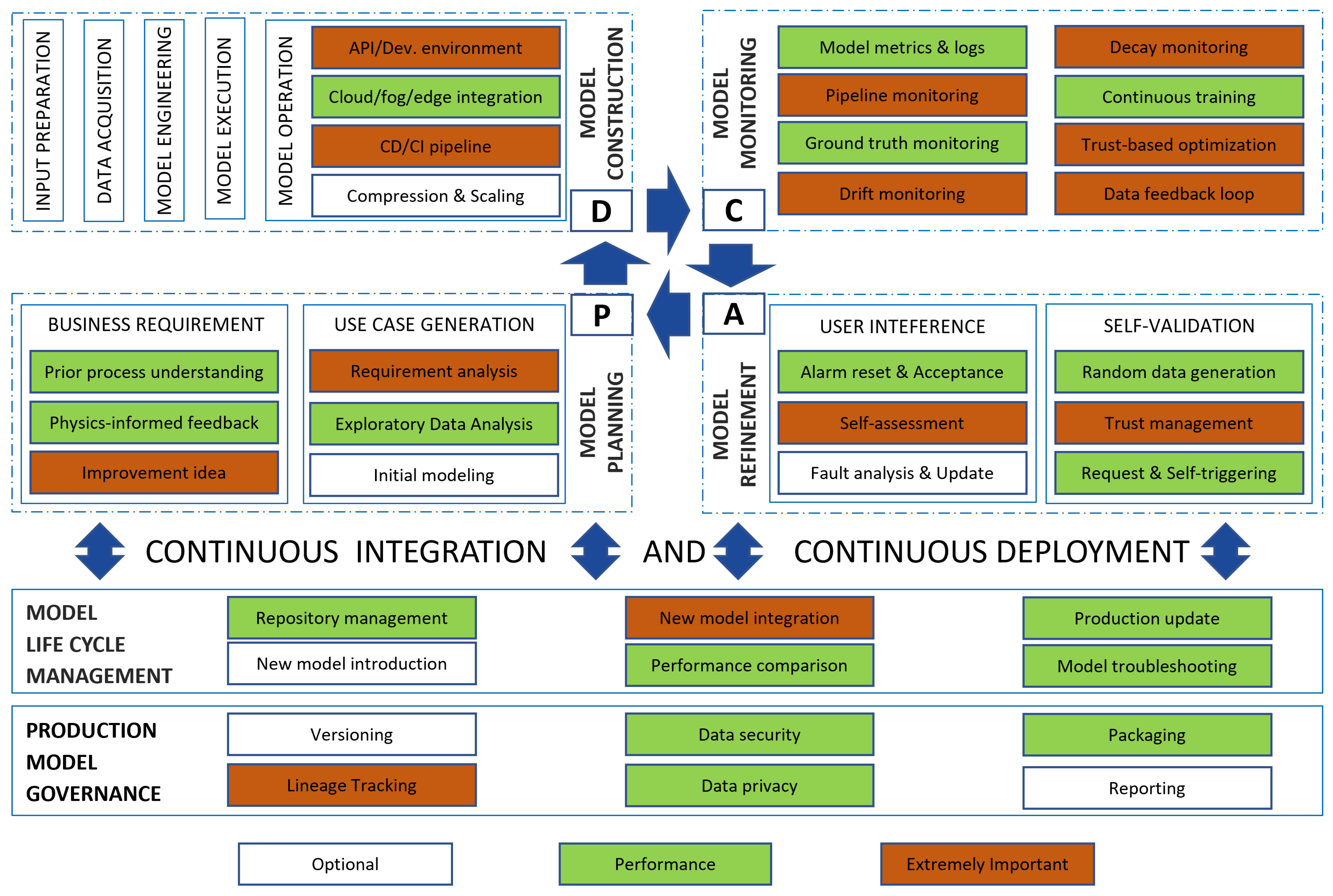
From the previous section, most of the XAI-integrated FDI research was focused only on the construction of the ML model, with very few hints for monitoring its performance or even less mention of the evolution of the model as a software product. However, an ML-powered software solution requires more extensive testing and monitoring than a manually-coded proof-of-concept system [80] and interdisciplinary collaborative effort from a team of stakeholders (such as process managers, business analysts, ML architects, data engineers, process engineers, and human end-users). This section contributed to the proposed MLOps principles that can be integrated into the development process of an XAI ML-based FDI solution, further adopting it into practical application. In the MLOps framework illustrated in Figure 2, two blocks in the upper center, “Model construction” and “Model monitoring”, are inherited from the previous section with the aid of the XAI concept and tools. To serve continuous integration and continuous deployment purposes [27,81], other blocks and phases are added to guideline software development activities. Based on this framework, stakeholders can work together during the development project. Noticeably, besides acting as a guideline, each task can represent the suggested requirement or desired feature for the ideal FDI solution product.
The same three-scale color code can be applied to indicate the importance of each step in this framework:
  • Extremely important: This step is critical to the continuous development and operation of MLOps.
  • Performance: This step is a basic requirement from the MLOps concept.
  • Optional: This step does not have significant importance and can be optional.
The concept behind MLOps is the continuous integration and deployment of incremental development with the ML model [82]. Therefore, considering the proposed framework as a feature guideline, the “Extremely important” features in red color are responsible for enabling the development environment (i.e., application programming interface (API) establishment), keeping the current version under stable operation (i.e., drift monitoring), and routing the output of the previous development into the input of the new model sprint (i.e., data feedback loop). “Performance” features prepare the necessities and architecture for each loop to be deployed (i.e., prior business understanding) while supporting the basic duties of an FDI tool (i.e., model performance metrics visualization). “Optional” features are not too critical for the efficient deployment of the MLOps loop; however, they complete the comprehensive automated development framework.
Several stakeholders take part in MLOps solution development, with overlapping responsibilities in some fields [83]. For simplicity, only the main players are proposed in this framework, whose practices are as follows:
  • A business stakeholder (BS) defines the goals of FDI tools and economic constraints. This role can represent the product owner, production director, quality manager, etc.
  • A data scientist (DS) is the translator between the business/process voice and ML/data problems with data-driven evidence.
  • A data engineer (DE) is in charge of data management, data solution, and data system architecture.
  • A software engineer (SE) works on the software architecture, including software-as-a-service and software-as-a-product management.
  • A machine learning architect (MLA) is the main designer of the ML model. They are in charge of any changes to the core algorithm and model during initial construction, update, compression, and scaling.
  • A DevOps engineer (DOE) bridges the gap between ML model development and FDI solution continuous development/deployment.
  • Human users (HU) stem from the requirement of the human presence in the ML-based product operation. Inspired by the work of [84], this role represents machine operators, maintenance engineers, process engineers, etc., whose work is benefited by using the FDI solution.
More details of these phases with associated tasks and corresponding stakeholders can be found in the Appendix A as a suggestion for task allocation in a FDI solution development project.
  • “Model planning” block: “Business requirement” and “Use case generation”
This is the first block in this framework, which is ignited before each Scrum sprint cycle. Its two phases, “Business requirement” and “Use case generation”, are equivalent to the “Business understanding” and “Data understanding” suggested in the CRoss Industry Standard Process for Data Mining (CRISP-DM) methodology [85]. In the “Business requirement” phase, new process requirements are sketched from the prior process/business understanding, as Meas et al. [54] suggested that knowing the financial consequences of the faults can motivate remedy actions. On the other hand, the model should be adjusted according to the facts acquired from the process via the physics-informed feedback loop or any improvement idea from the current process status. While the process understanding can be inferred from emerging business requirements [56] and improvement ideas are concluded from kaizen activities as proposed Awad et al. [86], the physics-related truth feedback loop can be established in the last step of the “Model monitoring” phase and provide the explored knowledge from the previous generalization performance [87]. This knowledge is necessary to build a physics-informed neural network [88]. A use case should be generated in the “Use case generation” phase to restrict the scope of the new desired feature and focus on key deliveries. The “Requirement analysis” step identifies the predefined functional and non-functional requirements, and the “Exploratory Data Analysis” (EDA) step should be conducted beforehand. An initial model is developed to check the feasibility of the new development loop [81].
  • “Model construction” block
Based on the outputs of the previous block, the “Model construction” and “Model monitoring” blocks will be carried out with support from XAI tools, as described in detail in the previous section. During the model operation sub-step, besides the model-related technical tasks mentioned above, several additional development-related tasks should be considered to facilitate the continuous delivery and integration of newly developed features [89,90], aiming at software deployment automation [91]. An “API/deployment environment” should be established with relevant infrastructure to run a service or application (app servers, databases, and caches) [30]. For convenient and efficient deployment, the model service can be deployed with “cloud/fog/edge integration” and a tailored design architecture [60]. A “CD/CI pipeline” and platform allow both the automation of data extraction and storage (for ML tasks) and the introduction of new version features within each development sprint (for MLOps tasks) [83,92]. The continuous deployment process can be automated with Jenkins [93] or Kubeflow, as proposed by Zhou et al. [92]. For effective deployment, each model should be compressed and optimized before scaling in the “Compression and Scaling” step. An API microservice with a container and an orchestration tool are generally required to build a scalable ML model [30].
  • “Model monitoring” block
During the “Model monitoring” phase, administrative tasks that keep track of new incremental improvements (i.e., model registry) should be carried out, with performance metrics measured in the “Model metrics and logs” step. Not only the performance of the model and the monitored system as mentioned in the previous section should be visualized, but the metrics related to the efficiency of the model as a software product (e.g., serving latency, throughput, troubleshooting time) [27,60] should also be considered. The “Pipeline monitoring” step ensures the intended data transformation and model performance, along with the consumed time and computational/data resources [92]. In some cases, a preliminary analysis of the raw signal during normal system operation to extract the ground truth is necessary [19]. Along with anomaly detection [94] in the “Ground truth monitoring” step, the “Drift monitoring” step recognizes the deviation from original usage (data drift, model drift, and concept drift) should be recognized and managed to adjust the predictive service level [95]. The concept of “Decay monitoring” with “Continuous training” [56,96,97] is recommended. As the XAI approach encourages the trust of human users in the model, “Trust-based optimization” is utilized with techniques to model human trust and workload during human–system interaction [98]. The “Data feedback loop” enables coherence between continuous sprint processes, while integrating prior and learned knowledge back into the network construction [78].
  • “Model refinement” block: “User interference” and “Self- validation”
Once the automatic operation and monitoring of the model have taken place, the “Model refinement” block is carried out. Though the ML approach can be automated, the contribution from non-ML expert users is suggested for the maintenance domain [33] or to measure the trustability of the model operation. In the “User interference” phase, action from human users can be resetting or elevating the alarm [18], performing “Self-assessment” on the usefulness of the results and suggestions from the model, with additional random validation supported by XAI tools [94], or even requesting a new model change [84]. Then, new knowledge can be derived based on the contemplating of the previous fault record in the “Fault analysis and Update” step. The model itself can be elaborated on with “Self-validation” features, in which test data can be generated and tested in the “Random data generation” step. This function is especially crucial for the case of imbalanced data [99], aligned with the tools deployed in the “Data augmentation” step in the “Model monitoring” block. As different users with different demands require different levels of information needs [100], the “Trust management” function should ensure a certain transparency level with personal preference for trust establishment [101]. This function works in tandem with “Trust-based optimization” in the previous “Model monitoring” phase. The optimization aim is to increase agreement between human users with the fault early alarm and suggestion from the FDI solution. Fault-related recommendations can be delivered with trust-based consideration on different users and scenarios [102]. The issues raised in this phase can generate requirements for the next model development sprint, starting with the “Model planning” phase.
Aligned with the famous plan–do–check–act (PDCA) cycle from the lean doctrine [103], these aforementioned four blocks can be regarded as P: “Model planning”, D: “Model construction”, C: “Model monitoring”, and A: “Model refinement”. This cycle constitutes the continuous improvement loop and exchanges information with two management blocks: “Model life cycle management” and “Production model governance”. These two blocks are not constructed in chronological order with the previous phases but are embedded from the beginning to create a comprehensive approach.
  • “Model life cycle management” block
Each model has a life cycle from the concept’s development until its realization resulting in a new version. Every change and footprint within its life cycle (under staging or production status) is recorded within the “Model life cycle management” block. In the “Model repository”, source codes should be uploaded in a shared storage location [30], where multiple developers and stakeholders can merge their work [83]. GitHub is a well-received hosting service for this collaborative coding purpose [104]. After being introduced into deployment from the “New model introduction” step, every model will be tracked within the “New model integration” during the gradual introduction and testing of features. The “Performance comparison” step compares the new model with existing ones using different strategies (e.g., recreate, ramped, blue/green, canary, and A/B testing [30]). Model approval in the “Production update” is required before being updated into production. The “Model troubleshooting” helps to reset the deployed model into the previous working version during operation.
  • “Production model governance” block
To comply with the forthcoming regulation for trustworthy artificial intelligence (AI) proposed by the European Union (EU) [105], the “Production model governance” block is inevitable to ensure limited risk during usage. This block verifies previous models deployed in production by corresponding tracking and audit activities in the “Versioning” and “Lineage tracking” steps, respectively. Relevant access control and security preference are handled in the “Data security” step, where each user has limited access and rights to interfere with and adjust information. Shahbazi et al. suggested the integration of blockchain technology into a distributed ledger layer to secure the data transaction between stakeholders via rest API [44]. The “Data privacy” step tackles personal data (e.g., personal trust level and preference) in compliance with laws and regulations (i.e., GDPR and CCPA). The model “Packaging and Documentation” step collects the required dependencies along with relevant product information with available package creation and management tools such as K8S [106] and Helm [107]. Last but not least, the “Reporting” step provides relevant documentation and materials for internal use.
The importance of each role is switched in different development phases depending on their knowledge and contribution to the development. For instance, BS and HU will have an important voice while shaping prior process understanding or improvement ideas, while SE and DOE need to pay attention during the lineage tracking and audit of the model.

3. Demonstration of the Approach in Hydraulic System FDI Monitoring

This paper expresses a comprehensive integration of XAI and MLOps concepts in developing an ML-based FDI solution. This section contributes to showing how relevant principles can be applied in a specific scenario. Although the use case does not provide all the proposed aspects, it helps to observe the importance of explanations throughout continuous model development: multiple incremental improvements and models have been developed, adjusted, and deployed. The authors focus on delivering a proof-of-concept demonstration in as many steps from the proposed framework as possible. With the proposed framework based on the conventional development of machine learning, integrated XAI and MLOps principles support an explanation with relevant reasonings in every development step of a continuous development and integration cycle. Based on these principles and guidelines, the team working on this FDI solution-development project can obtain maximum efficiency with a high consensus and the least amount of confusion.

3.1. Description of the Use Case

As the industrial data source with authentic time series from manufacturing lines is scarce, an online-available experimented data set from a hydraulic test rig [108] is utilized, as hydraulic systems are a good representative of complex non-linear industrial systems. The concerned system, consisting of a primary working and a secondary cooling-filtration circuit, is described in Figure 3, with 17 raw sensor signals collected in which 14 are process-measured sensors (six pressure sensors, one motor power sensor, two volume flow sensors, four temperature sensors, and one vibration sensor) and three are virtual sensors (one efficiency factor sensor, one virtual cooling efficiency sensor, and one virtual cooling power sensor).
The number of cases is 2205, with 43,680 attributes per measurement, with seven sensors operating with a sampling rate of 100 Hz, two operating at 10 Hz, and the last eight sensors having the rate of 1 Hz. Each case represents a working cycle that lasts for 60 s. Characteristics of the input signals from each sensor are summarized in Table 1.
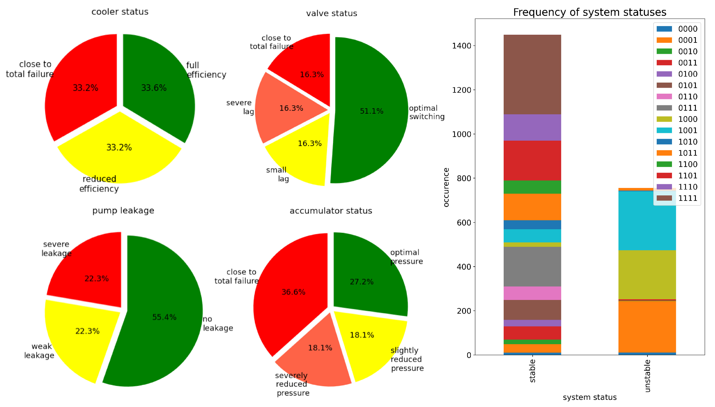
Generally, the system has two operating states of stable/unstable (with 1449/756 instances, respectively), which can be designated with 0 and 1, respectively. If 0 and 1 values are used to designate the normal and faulty state of each component, respectively, the fault status of the system can be represented by the vector y = [ s m ] , with s m ( m = 1 M ) representing the operating status of m-th component, where s m 0 , 1 . For example, the vector [ 0001 ] represents the faulty status of the fourth component, while the first three components function normally. Different fault grades of these components are sorted in order of severity as follows:
  • Cooler (three grades): 1: full efficiency, 2: reduced efficiency, and 3: close to total failure ( 741 / 732 / 732 cases, respectively).
  • Valve (four grades): 1: optimal behavior, 2: small lag, 3: severe lag, and 4: close to total failure ( 1125 / 360 / 360 / 360 cases, respectively).
  • Internal pump (three grades): 1: no leakage, 2: weak leakage, and 3: severe leakage ( 1221 / 492 / 492 cases, respectively).
  • Accumulators (four grades): 1: optimal pressure, 2: slightly reduced pressure, 3: severely reduced pressure, and 4: close to total failure ( 599 / 399 / 399 / 808 cases, respectively). These grades are artificially stimulated by four accumulators (A1–A4).
The ratios of each fault grade within each fault type are shown in Figure 4.

3.2. Traditional FDI Approach with an ML-Based Model

There were previous attempts to perform FDI tasks on this dataset. The traditional condition monitoring proposed by the author used linear discriminant analysis (LDA), artificial neural network (ANN), linear SVM, and radial basis function SVM to classify the fault condition and grade of severity [35]. The segmentation of each cycle into 13 segments based on the valve operation was not described in detail. The original approach extracted 20 features based on Pearson and Spearman correlation analysis from a large number of 1323 and 1197 available features in time and frequency domains, respectively. The authors also visualized the effect on classification rate by various numbers of regression cycle windows and various numbers of features. Adaptive linear approximation (ALA) and recursive feature elimination SVM also improved the classification accuracy [36]. Regarding model performance monitoring, sensor faults that can lead to false alarms (i.e., constant offset, drift, noise, and signal peaks) are compensated for by the feature extraction method [109] and fed into a kNN classification in an LDA-reduced space. A combination of a DL model and wavelet packet decomposition is suggested by Wang et al. to address both single-fault and multi-fault classifications [37] and t-distributed stochastic neighbor embedding (t-SNE) is deployed to visualize the learned features. A deep neural network (DNN) classifier with feature contribution explained by DeepSHAP was proposed by Keleko et al. [38]. The authors suggested that feature selection can be carried out based on these results, without going further into the continuous tuning and deployment approach.

3.3. FDI Model with a LSTM Neural Network

The previously presented achievements do not interfere with the scope of this study, which is the development of an ML-based FDI solution with the aid of XAI and MLOps principles. This data set is suitable for reflecting many aspects suggested in the previous sections. This section highlights the suggestions for using these two concepts during development to emphasize their potential. As the relevant input data in FDI problems are usually acquired from sensors in the form of time series, an LSTM neural network is a favorable candidate to detect anomalies from the baseline [110] and enable early detection [24,111]. An LSTM neural network is proposed as the core ML algorithm to develop a multi-class classifier for FDI applications due to its flexibility and capability in classifying, processing, and making predictions based on time series data of nonlinear dynamic systems.
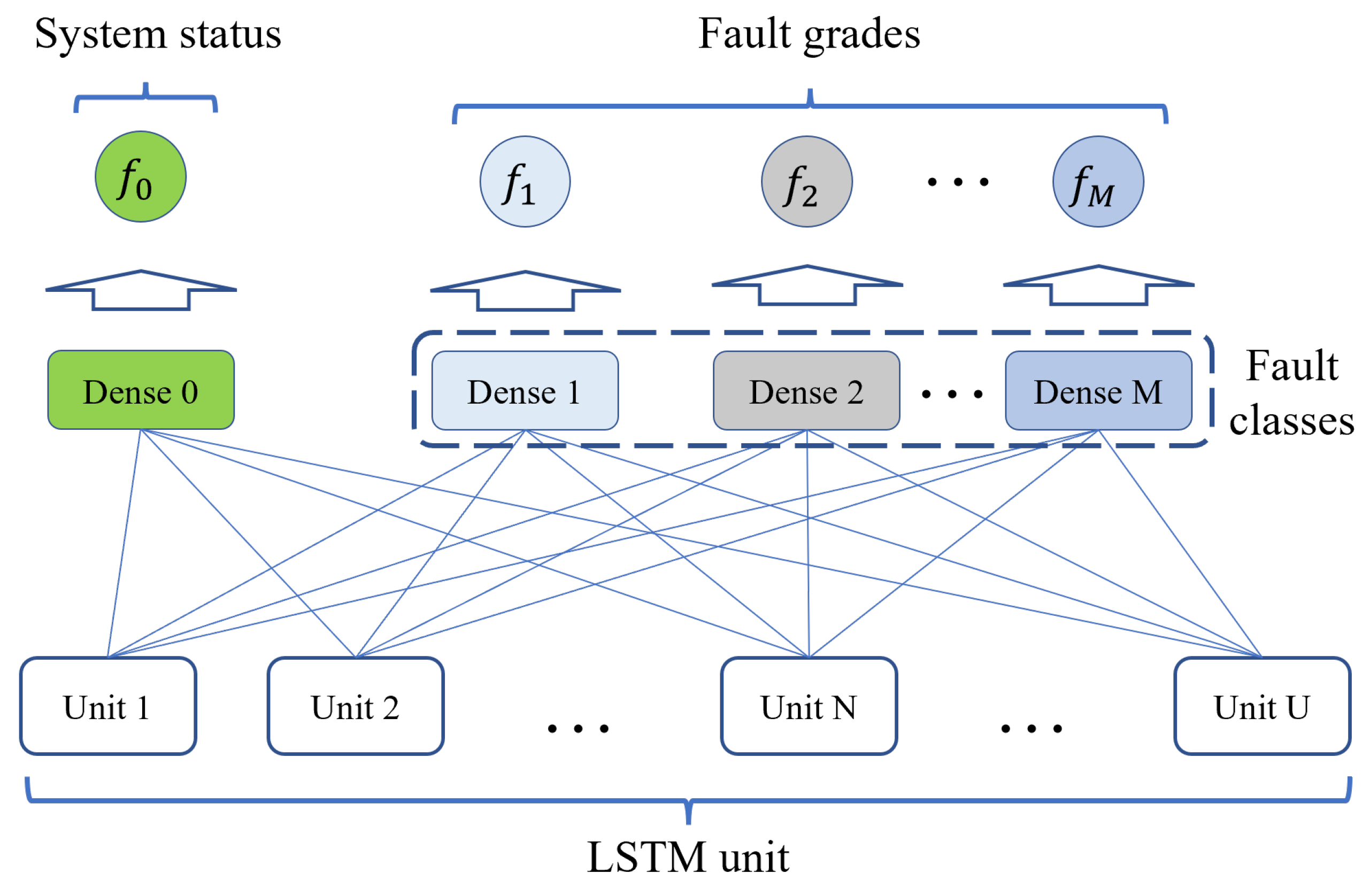
The FDI problem can be formulated as event sequence forecasting [112], as LSTM memory cells will hold the information they learned in the previously input time steps. The architecture of LSTM for FDI solution can be seen in Figure 5, with the matrix X = [ x i ] ( i = 1 N ) representing the components of the input sequence, where each component is a continuous-valued representation with N elements. H = [ h u ] ( u = 1 U ) represents the components or “hidden variables” of activities from U LSTM units. The number of U does not necessarily equal the length of N and can be subjected to change, but it is recommended that U N , thus receiving the full information from the input sequence. Then, a neural classifier in a dense layer is trained to calculate the probabilities from all LSTM units. This principle applies to both classifying the system status between the stable/unstable value and then classifying the status of each component. The output of the dense layer is P ( f | X ) = P ( f c ) ( c = 1 C ) , where c can be the number of system status or the number of fault grades within a f fault class:
P ( f | X ) = P ( f | H ) = e x p ( H T w c + b ) c = 1 C e x p ( H T w c + b ) ,
in which w c is the c-th column vector of the W o matrix of the output layer of the network, and b is the bias vector of the neurons. The class label with the highest probability is considered as the predicted status or fault y ^ :
y ^ = max c P ( f | X ) .
To get an insight into how each LSTM unit took part in the decision on fault type, a scheme of one cell is illustrated in Figure 6.
It can be seen that this N t h cell receives the activation h N 1 and state C N 1 from the previous ( N 1 ) t h cell and the x N from the input sequence. The state of this cell will be updated based on the forget-gate f N and filtered input gate i N :
C N = f N C N 1 + i N C ˜ N 1 ,
where
f N = σ ( W f [ h N 1 , x N ] + b f ) ,
i N = σ ( W i [ h N 1 , x N ] + b i ) ,
C k ˜ N 1 = t a n h ( W c [ h N 1 , x N ] + b c ) ,
where b is the bias vector of the neurons, and σ and t a n h are the applied sigmoid and tanh activation functions, respectively. W f , W i , and W c are the weight matrices of the forget gate, input gate, and cell input of the cell, respectively, which need to be learned during training. The activity of this LSTM unit is then calculated from the cell-state C N and the output gate signal o N :
o N = σ ( W o [ h N 1 , x N ] + b o ) ,
h N = o N t a n h ( C N ) ,
where W o is the weight matrix of the output gate. PCA is then performed on the matrix H T = [ h u ] T , where [ h u ] = [ h 1 , h 2 , , h U ] and is used to map the activated weight from U LSTM units into a two-dimensional space while keeping the most important information. The new data points after PCA are as follows:
S = H T × W = [ h u ] T × W ,
where S = [ s ] is the output of PCA, and W is the U × 2 dimensional eigenvector matrix of weights, whose columns are the eigenvectors of H T H . The C different fault grades of the f fault class should form corresponding distinguishable areas within the new two-dimensional space, as this increases the chance that correct identification can be performed. This arranging after PCA can be assessed by metrics such as the Davies–Bouldin index:
D B = 1 C a = 1 C b = 1 C max a b ( S a + S b d a , b ) ,
where C is the number of fault grades, and S a and S b are the average Euclidean distances of every data point < x > and < y > within fault grades a and b to their corresponding centroids C S a and C S b , respectively.
S a = 1 N a x S a x C S a 2 ; S b = 1 N b y S b y C S b 2 ,
where N a and N b are the number of samples within fault grade a and b. d a , b is the absolute value of Euclidean distance between the centroids of fault grades a and b.
d a , b = C S a C S b .
The case of an FDI solution for a system with multiple fault classes, where each class has various fault grades, is illustrated in Figure 7, with m fault grades predicted from corresponding m dense units. A separate dense unit is reserved to predict the system status (either the operating status of stable/unstable or the low-level status of y = [ s m ] , or the users can use two separate Dense units for predicting both).

3.4. Explainability during FDI Model Development

As XAI tools are intended to create a continuous tuning and improvement loop, in this section, the adjustment of each phase during the “Model construction” block will be presented along with the corresponding phases during the “Model monitoring” block, considering the reasoning provided from the visualized results. In addition to the recommended tools in Table A1 and Table A2 in the Appendix A, new tools are also demonstrated by the authors. After training and cross-validation, the structure with the best-performed prediction is utilized as the fault detector.

3.4.1. “Data Acquisition” and “Pipeline Development”

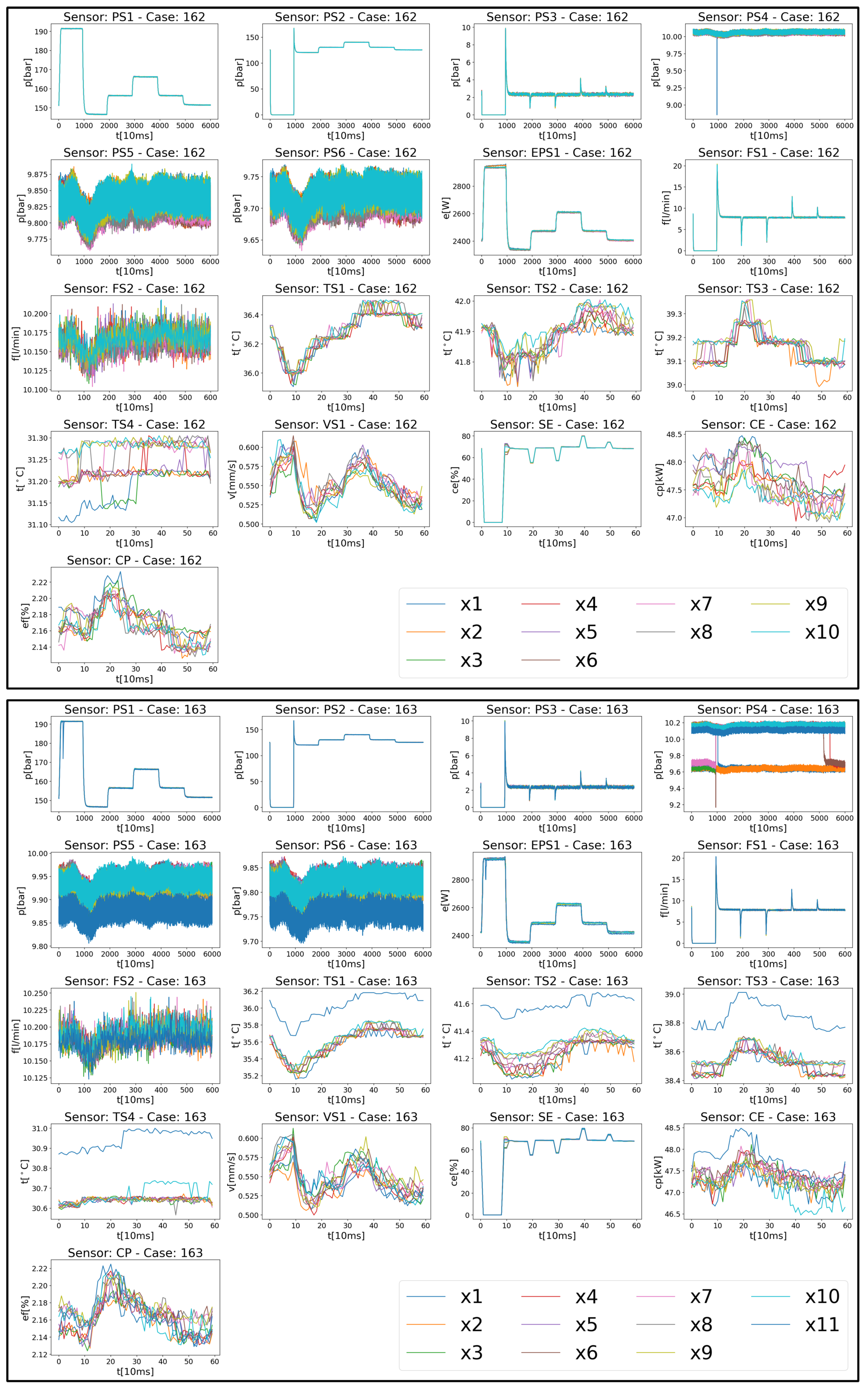
This data set was already collected from a test rig; therefore, the “Data acquisition” step is not mentioned in this study. However, the tools mentioned in Table A1 can also be applied for a better understanding of human users, such as in the “Sampling frequency” and “Data annotation” steps. The “Data augmentation” step can be carried out with SMOTE, as the data set is imbalanced after considering the data annotation table [38]. In “Fault definition”, the baseline of sensor data and each typical fault can be stored, with 17 associated input signals from cycles yielding the same system status. Figure 8 shows two typical operating modes, where there is no fault happening among the critical components, with the data distribution and signal patterns from such cycles. One operating mode yields a stable status, while the other reflects that the system is not stable yet. These data serve as the baseline of sensor readings for later quick fault recognition using statistical parameters (mean, median, etc.) to detect abnormal signals that exceed conventional intervals. When a new prediction is made in the “Model operation” phase, its associated signals are compared with the corresponding references to support the later root-cause analysis.
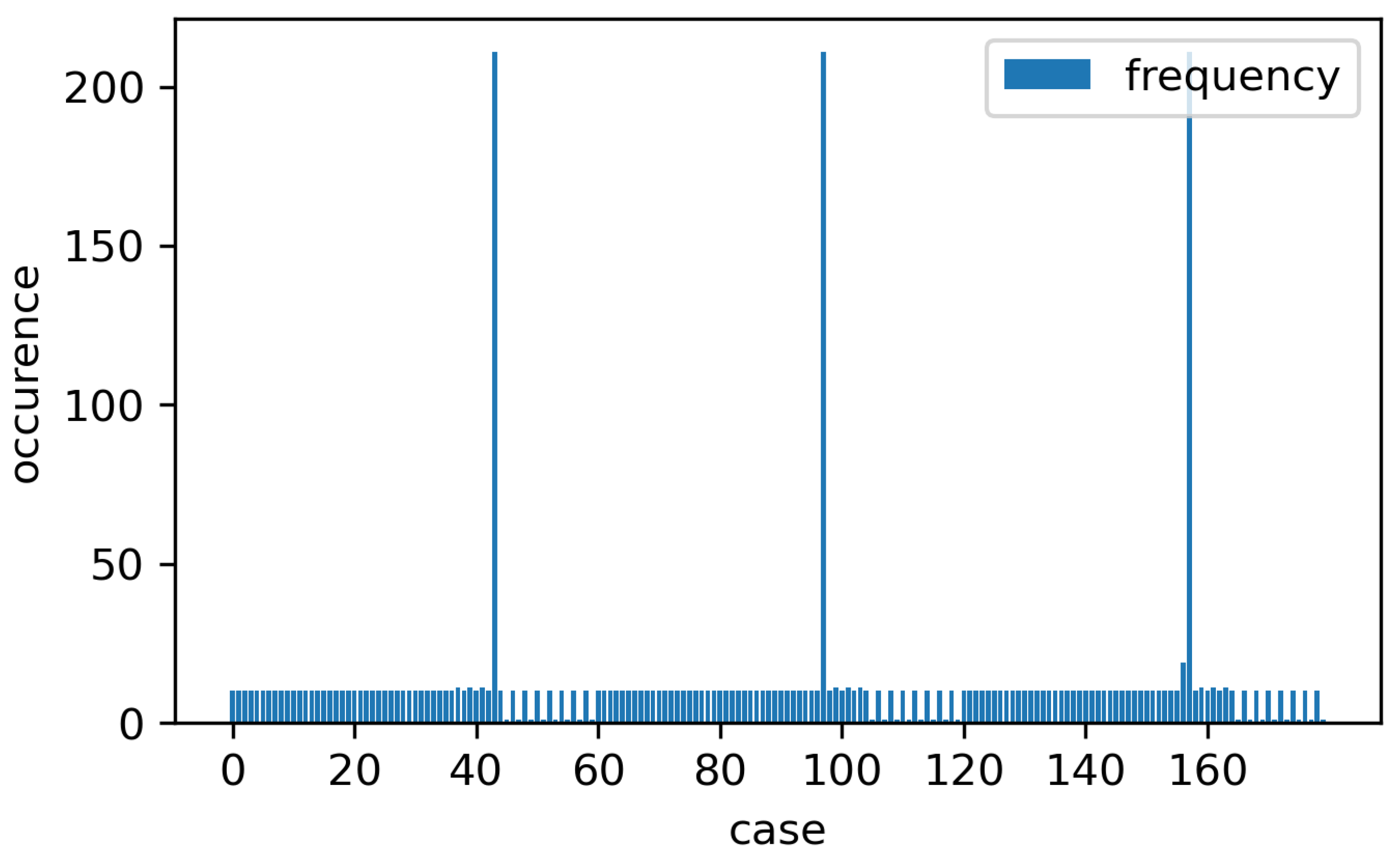
In “Input data management”, the number of total cases with their frequency can be visualized as a moving window during operation, as shown in Figure 9. This window will be updated after each prediction. The monitored system is assumed to work normally when new fault cases appear with acceptable frequency. If the frequency of a fault exceeds a certain threshold, the working condition could have drifted, and a warning can be given.

3.4.2. “Input Preparation” and “Input Sufficiency”

The operation of the whole system depends on the pre-defined load from the pump, which generates the pressure value on sensor PS1 during fixed time intervals in every working cycle. The segmentation of raw input data was not mentioned in the original work [35]; however, this is an important step to extract features from all sensor data and should be monitored. Considering the number of intervals within a working cycle is fixed as 12, the problem becomes detecting a known number of K = 11 change points within a given signal y ^ = y 1 y T = y t t = 1 T . Choosing the best possible segmentation τ then equals solving a discrete optimization problem [113]:
min τ = K V ( τ , y ^ ) = min k = 0 K c ( y t k y t k + 1 ) ,
where c ( . ) is a cost function that measures the homogeneity of a signal segment y t k y t k + 1 according to a chosen signal model, which will be low if this segment does not contain any change point, and vice versa. Different signal models can be considered according to specific use.
In this use case, the different automated segmenting methods with the corresponding raw input signal before and after segmentation are visualized in Figure 10, with the defined threshold K = 12 applied for another sensor signal for reference. The available packages that can be deployed are stumpy [114], BEAST [115], seg1d [116], or rupture [117] with offered models. Once a package is chosen, for example, rupture as in Figure 10, dynamic programming is chosen as the optimal detection method, along with the cost function c ( . ) . The user can see the different preferences of the change point detection algorithm between them and choose the most useful one.
Although many features are proposed in the original study, the purpose of this study is to demonstrate the feasibility of the proposed frameworks; therefore, only the mean value of each signal segment is considered to build a compact FDI model. Corresponding to the mean value of 17 sensors, there are 17 features associated with each segment. If necessary, new features can be incorporated after the first iteration of model construction when observing the train and validation accuracy and calculating the feature contribution [38]. In the “Data transformation” step, scaling is carried out with the power transformer from the Scikit-learn package [118].
During the “Input preparation” step, a Gantt chart can be deployed to visualize the block design. The number of blocks and the separation between each block can be adjusted as a hyperparameter of the model. Considering that different fault types have different distributions of degradation levels, the block design should make an equal contribution to these levels. The block length l b can be considered as follows:
l s l b l f ,
where l s is the duration of the shortest stable faulty period, and l f is the duration of the longest fault fluctuation. The maximum block length can be defined within the sweet-spot region based on the regression requirement from the fault type, the data limit, and the computation limit [119]. The duration of block separation l s e p is considered by the following:
0 l s e p l s .
The blocks can be separated from each other with a positive value of l s e p , but not too far, as this skips the gap of l s . Then, the number of blocks n b is calculated from the total number of samples N s :
n b = N s l b l s e p .
Some samples can be removed from the dataset; thus, the numbers of samples in blocks are even or the final block may have fewer samples than the other. Figure 11 shows the intended blocks along with the degradation levels of four fault classes. To utilize the existing amount of data, zero separation was set. It can be seen that the block length is longer than any stable regions within the fault of the accumulator condition but does not exceed the length of the last fluctuation at the end of the valve condition. The distribution of these blocks can capture the status changes within the condition of the cooler.
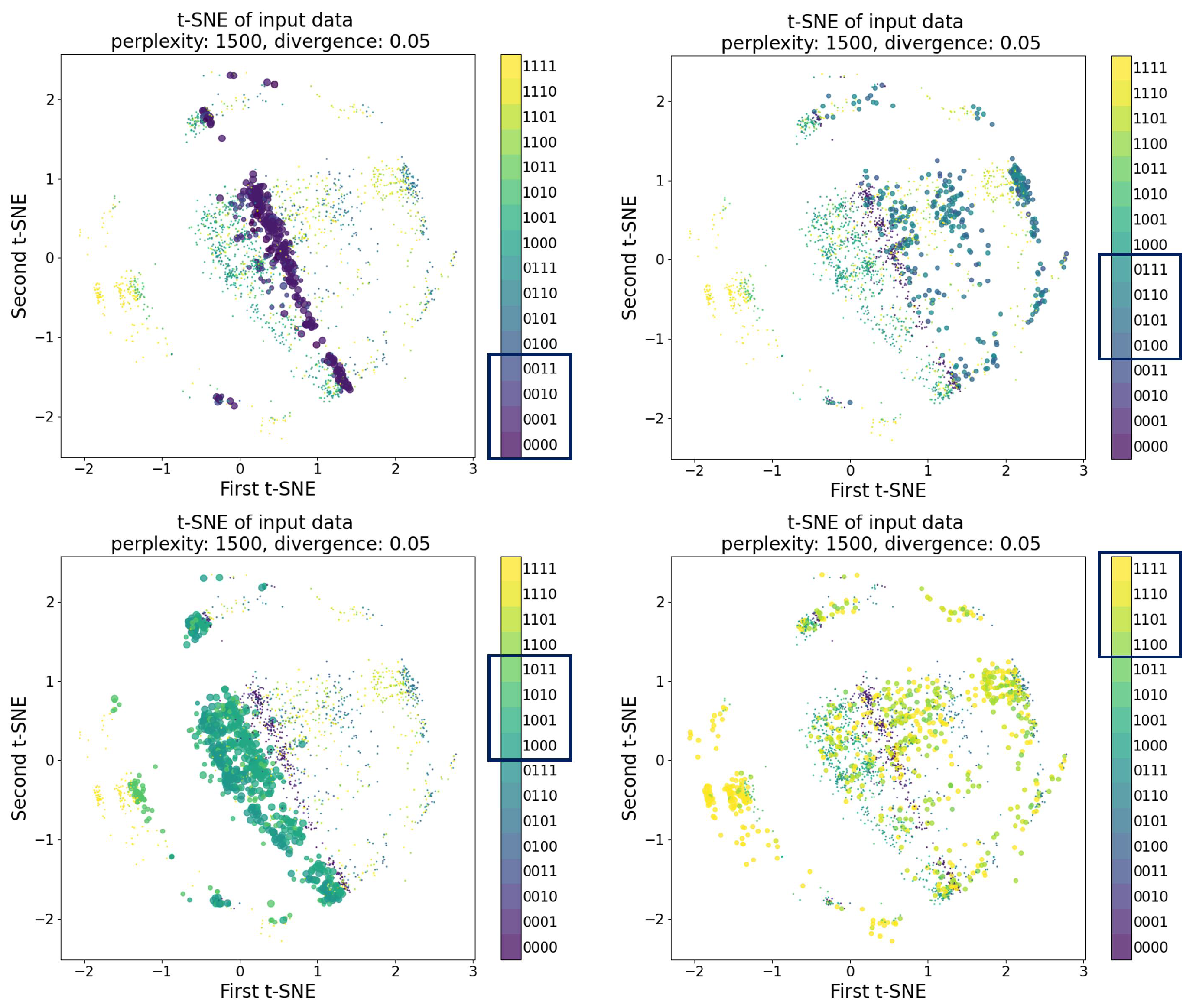
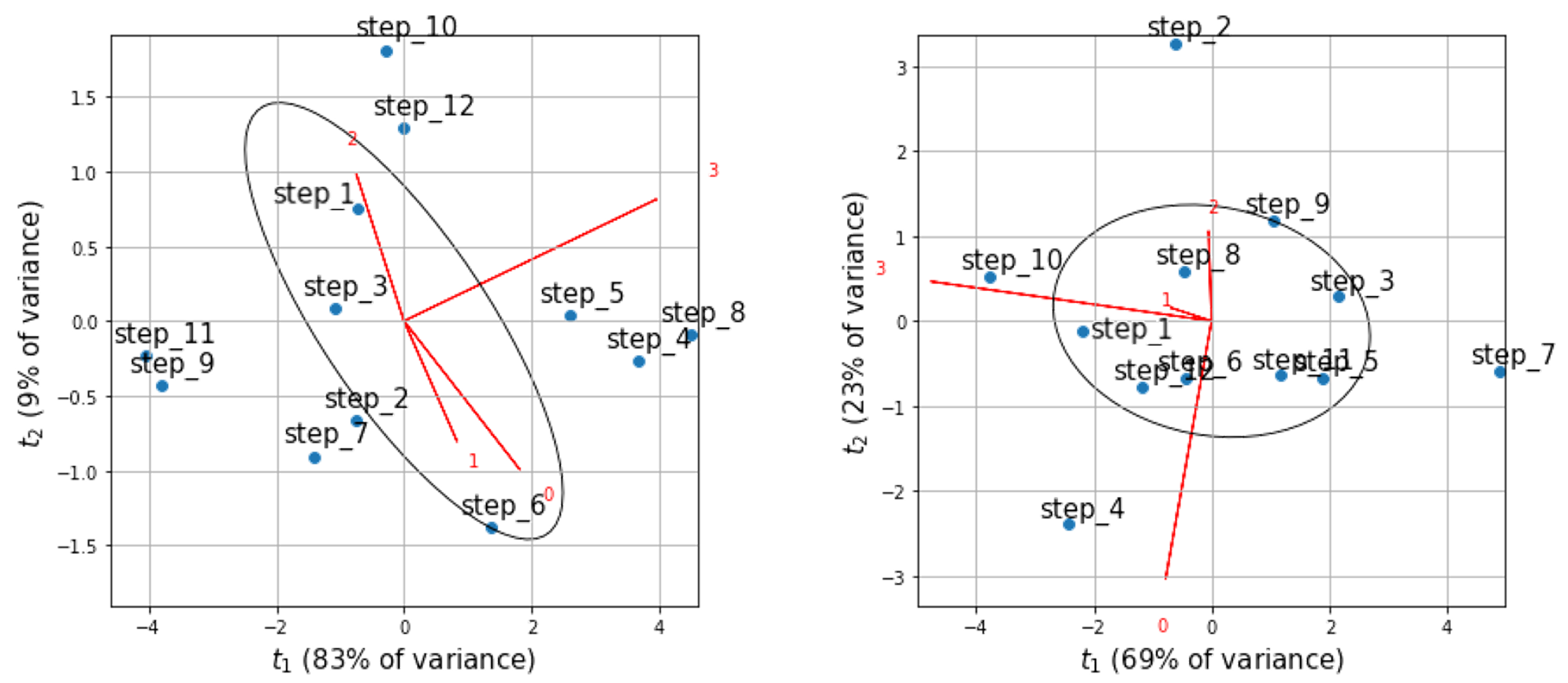
Conventionally, input data from sensors in FDI problems are high-dimensional. The input space regarding fault annotation can be diagnosed with dimension reduction tools (e.g., PCA and t-SNE [120]) to understand the dispersion of the input data, as well as choose the features characterizing the separation of faults. As an operating cycle is segmented into 12 intervals and the original authors of the dataset suggest using five statistical features for each segment [35], the dataset ended up with 5 × 12 × 17 = 1020 features, in which 17 is the number of sensors. By analyzing the PCA result on this maximum number of original features, the most important features can be recognized based on their loadings for each principal component, as illustrated in Figure 12. By selecting a suitable set of the most important features from the original set and even in combination with the transformed set after PCA, the users can adjust the distribution of data in the input space to obtain the best explanation of the system status or fault grades according to their needs.
In Figure 13, different system statuses show different distributions in the input space, but the influence of the first and second components (i.e., the cooler and the valve) can be easily observed.
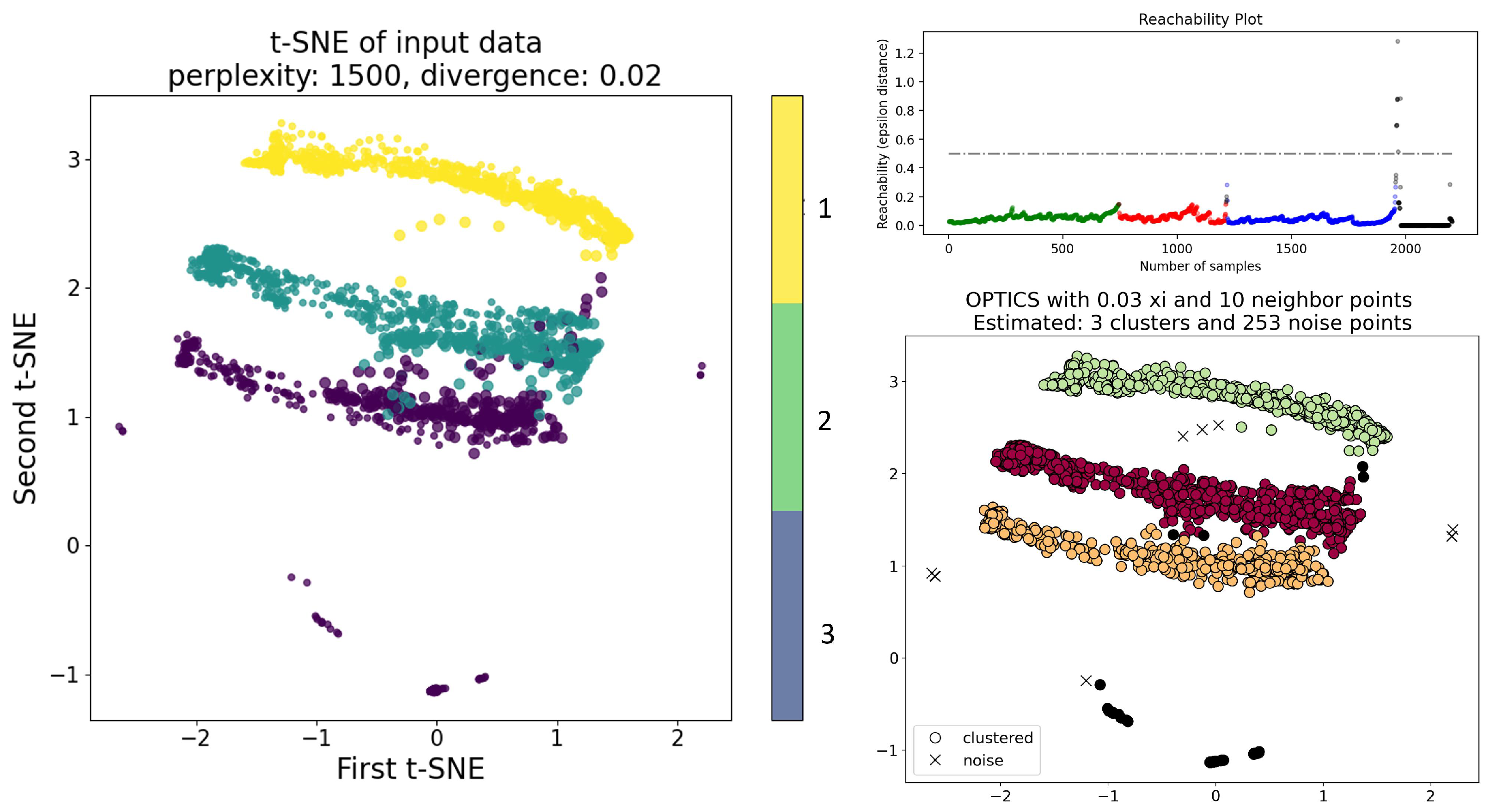
Once good separation of a certain fault class in the 2D space is achieved by fine-tuning the t-SNE, density-based clustering algorithms (e.g., DBSCAN, OPTICS [118]) can be applied to detect the noise and outlier data points. The users can adjust the hyper-parameters of these algorithms with the visualization of Euclidean distance within data points, as illustrated in Figure 14. Abnormal input data can be detected in this early phase [74].
Later in the “Diagnostic capability” step, the same analysis can be applied to the output data, and then the difference between the two analyses shows the distance preservation capability of the model.
“Regression consideration” and “Regression sensitivity” work in tandem, as illustrated in Figure 15. Based on the learned weight of the dense layer before each fault output along the LSTM unit, different time steps have different effects on each fault type. ML engineers can consider adjusting the regression in each fault branch with separated LSTM layers, which can be modified in the “Model engineering” step. Since the system operation and system status will always be predicted with separate dense layers, from now on, we only discuss modifying the architecture of the LSTM layer to better predict the fault in each component. The accuracy of prediction on each fault is then measured against different lengths to suggest the best regression step. It can be seen that with the first fault grade of the cooler, the ninth lagged time step does not contribute toward prediction.

3.4.3. “Model Engineering” and “Structure Sufficiency”

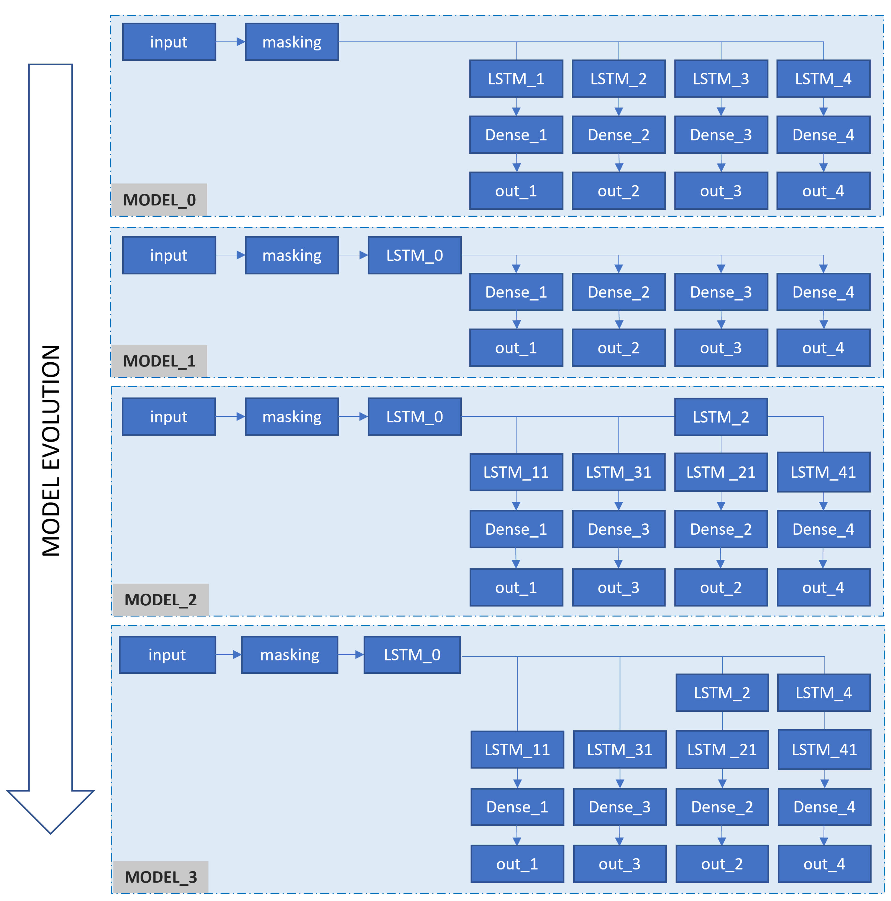
Considering that the transition phases are excluded from this data set [35], a classification model is chosen over the regression one, as also adopted in the study of Keleko et al. [38]. In previous research, authors usually suggested choosing an appropriate model from several trained models. In this research, we focused on adjusting the classification model based on the core LSTM layer by performing simple and incremental improvements. We suggest the use of the functional API of Keras [121] for this purpose. The incremental improvement of the model structure will be described, with an example illustrated in Figure 16.
Model evolution starts with a simple model with a single input and multiple outputs (Model_0), predicting each fault type by separated LSTM branches for each fault. Although only the mean value of each sensor during a segment is used as the only feature, Model_0 yields a modest result. Model_1 is more compact as it uses a single LSTM layer for all fault types. After training and validation, the first fault type from the first output (out_1) reaches a sufficient accuracy level; however, the other faults have inaccurate training accuracy. Based on the visualized accuracy of each fault type, the model can be adjusted by adding mode LSTM layers to the fault types that require more accuracy. The second structure evolution (Model_2) then has one more LSTM layer (LSTM_2) in the branch of the other two outputs (namely out_2, and out_4). Because the LSTM_0 needs to return its sequence to the newly added layer, additional LSTM layers with one unit should be added before each dense layer (LSTM_11, LSTM_21, LSTM_31, and LSTM_41). The iteration can continue to Model_3, as the LSTM_4 layer can be added in the branch of the fourth fault prediction (out_4). The LSTM_0, LSTM_2, and LSTM_4 layers can have their lagged time-step adjusted based on the “Regression consideration” step. This approach makes it easier to adjust and modify the ML structure with simple evolution steps.
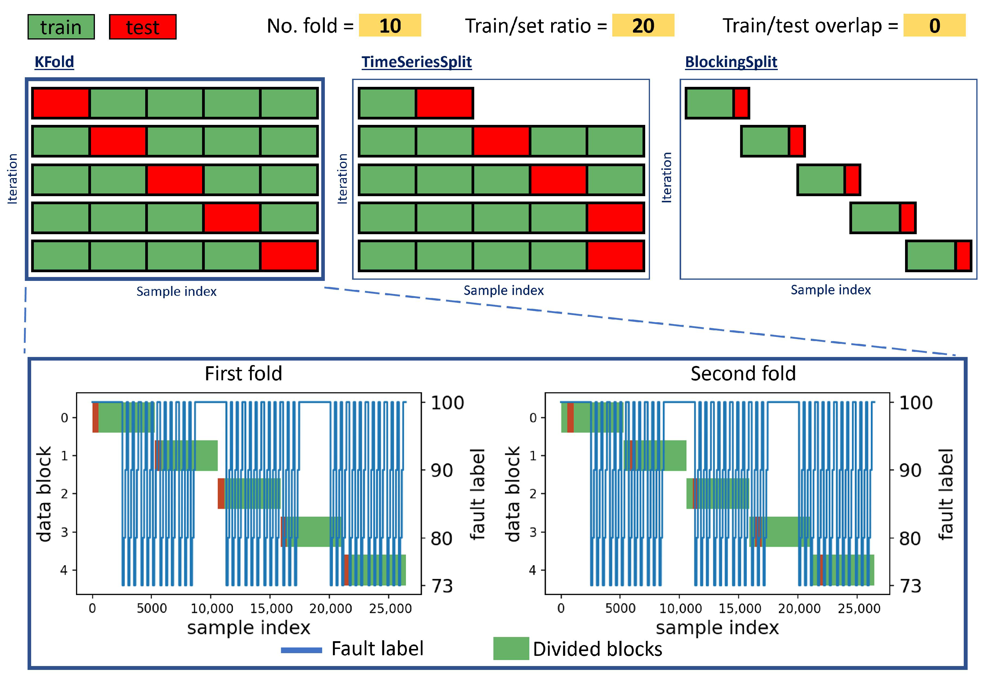
Within each block determined in the previous step, the train and test set along with the validation strategy should be defined. Visualization of different validation strategies is proposed in Figure 17. Thanks to the flexibility of the Scikit-learn package [118], different splitter tools can be designed; therefore, the validation strategy can be adjusted according to the fault characteristics. The number of folds, the ratio between train–test sets and the associated overlap, and the starting sample index are shown and allow users to define a customized validation strategy.
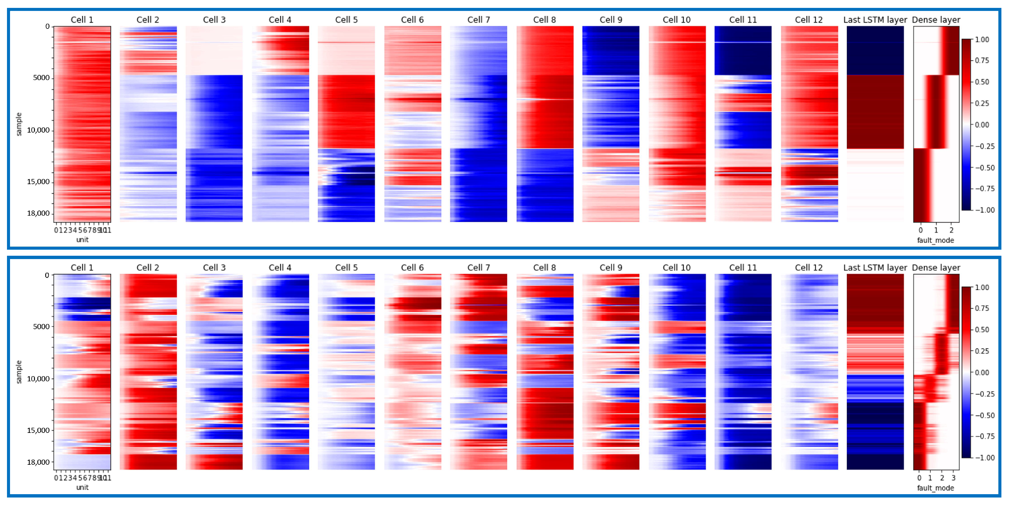
The activation value of the LSTM layers associated with one fault branch illustrates how each layer learns from the input data set. In Figure 18, the first and fourth fault branches from Model_3 are visualized. The first branch consists of LSTM_0, which contains 12 cells, and the LSTM_11 has one cell. The Dense_1 layer is the last; however, the fault grade is already well-shaped in the last LSTM layer. From this visualization, the effect of the number of LSTM units can be studied considering the fault grade. In this figure, the third cell did not contribute to the prediction of the third fault grade of the first fault, as the white color indicates zero values. In addition, the number of cases the model required to learn a fault grade can be inferred based on the pattern of activation values: if the pattern does not change in all the cells, this means the model has stabilized. The LSTM_4, LSTM_41, and Dense_4 layer activations are shown in the fourth branch. It can be seen that the learning efficiency of the second and third grades of the fourth fault is not good, it is 92 % . The same visualization also serves decision trajectory tracking during the “Model operation” phase. An abnormal activation pattern means a new fault appearing or the model is degrading.
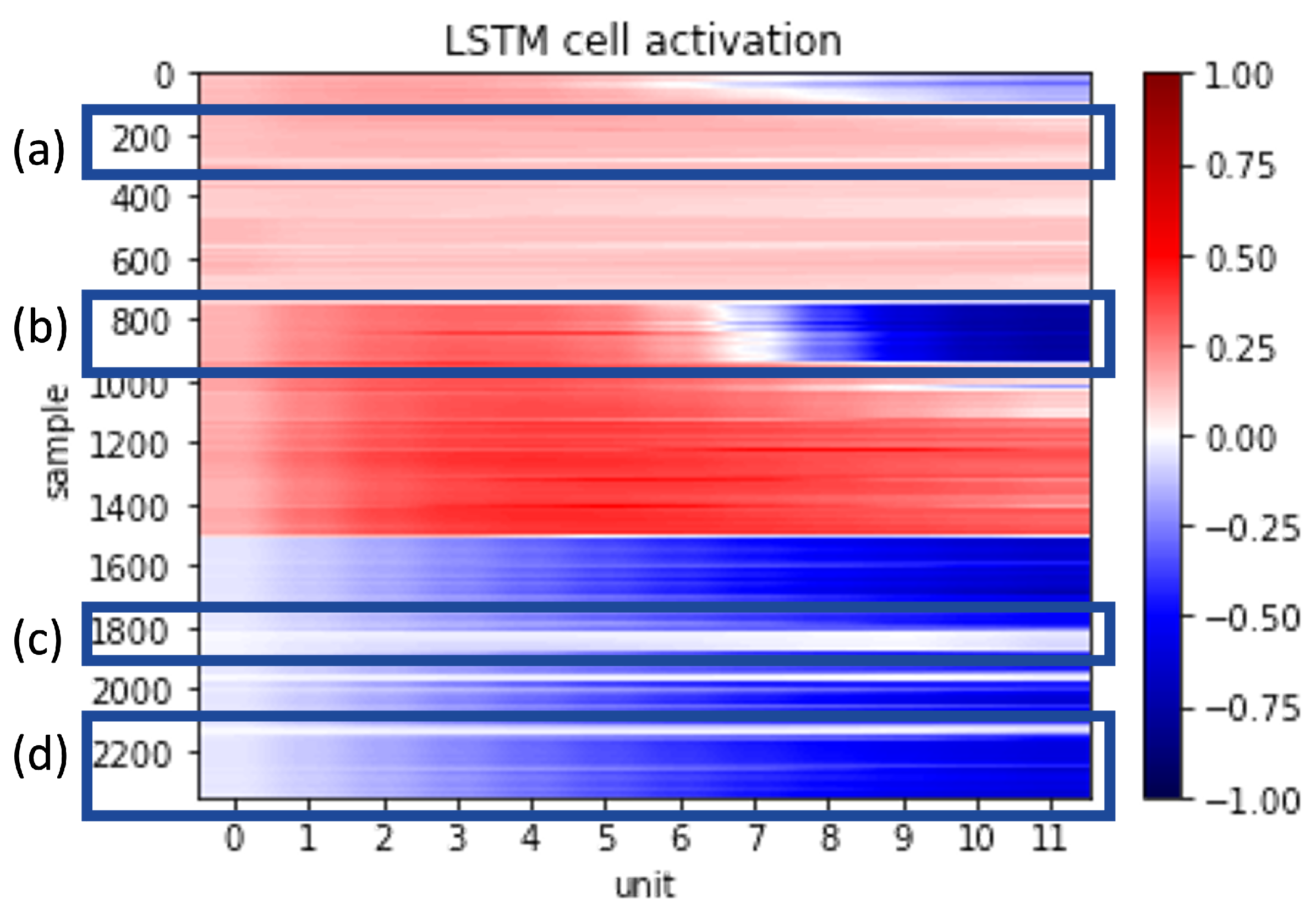
A closer look at the activation value of an LSTM cell can be used to analyze how the model learns from a fault, and how the fault grades are separated in each cell, as inspired by the work of [112]. In Figure 19, four behaviors of LSTM cell activation can be observed: remaining at a constant value, reversing the value, remaining at a neutral value, and changing from a neutral value. These behaviors reflect the learning capability of the model according to the regression time step. For instance, the (b) behavior will be missed if only seven regression time steps are considered.

3.4.4. “Model Execution” and “Decision Rules”

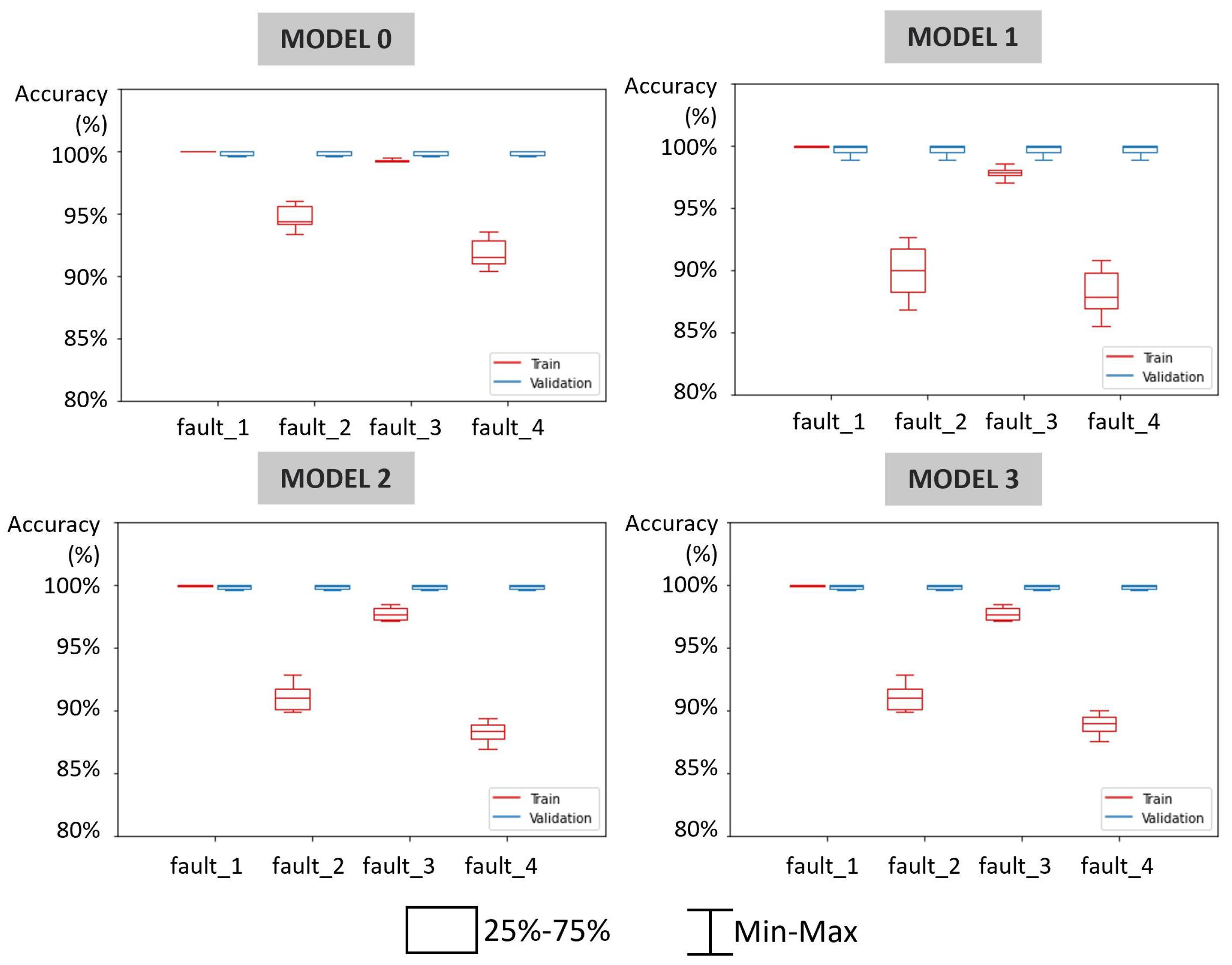
To select the suitable model architecture, the “Train and Validation accuracy” of each fault type within the first four models are shown in Figure 20. Model_0 has adequate accuracy, as each fault type is learned separately within each branch of the LSTM layer. Model_1 is more compact, as all four types are learned by a shared LSTM layer, but it shows wide accuracy variation during training of the last three fault types given the fact that each fault type has a certain effect on the decision space. Improving the learning performance but still maintaining compactness by gradually adding more LSTM layers in the fault branch helps to reduce variation, as discussed in the previous “Model engineering” phase. Noticeably, due to the limited amount of data and the relatively simple characteristics of the faults, all models achieve better performance in the validation set compared to the train set.
The “Feature contribution” step can be conducted with DeepSHAP [38]; therefore, it is not repeated in this use case. The analyzed result can be used to choose relevant sensor signals during the “Pipeline development” step. The confusion matrix of Model_2 is shown in Figure 21. Although system operation between stable/unstable is well-predicted, the model experiences some confusion when predicting system faults. This model has an extra LSTM layer dedicated to both learning the second and fourth fault types; however, it can be seen that while the model achieved a decent result with the second fault, it still has a poorer performance with the fourth fault.
Decision trajectory tracking can be carried out with PCA applied to different cells of an LSTM layer in a fault branch. Considering PCA as a projection operation, this trajectory tracking can visualize how the model tries to separate the fault grades. In Figure 22, PCA is carried out on five cells of the LSTM_0 layer of the first fault branch. From the very first cell, the three fault grades are mixed. Until the eighth cell, they are separated but not concentrated. Therefore, the model tries to converge them in the tenth and twelfth layers but only succeeds with the first and second fault grades. The third one is still distributed sparsely. However, this separation is enough for the classification in the last LSTM layer, as one dimension is already sufficient to describe the data variation, and PCA cannot be applied in this layer.
However, in Figure 23, which visualized the second fault branch, as there are four fault grades, the PCA projection needs to separate all these fault types in the last LSTM layer of this branch.
By applying PCA on the weight of the last LSTM layer [112], the weight of each time step and the eigenvectors can also be visualized, as in Figure 24. It can be seen that with different fault types, different time steps yield different influences on the PCA result, which indirectly affect the classification ability of the model. By analyzing the distribution of these weights, the importance of each time step to the prediction of each fault type can provide a better understanding of the time behavior of the fault.

3.4.5. “Model Operation” and “Diagnostic Capability”

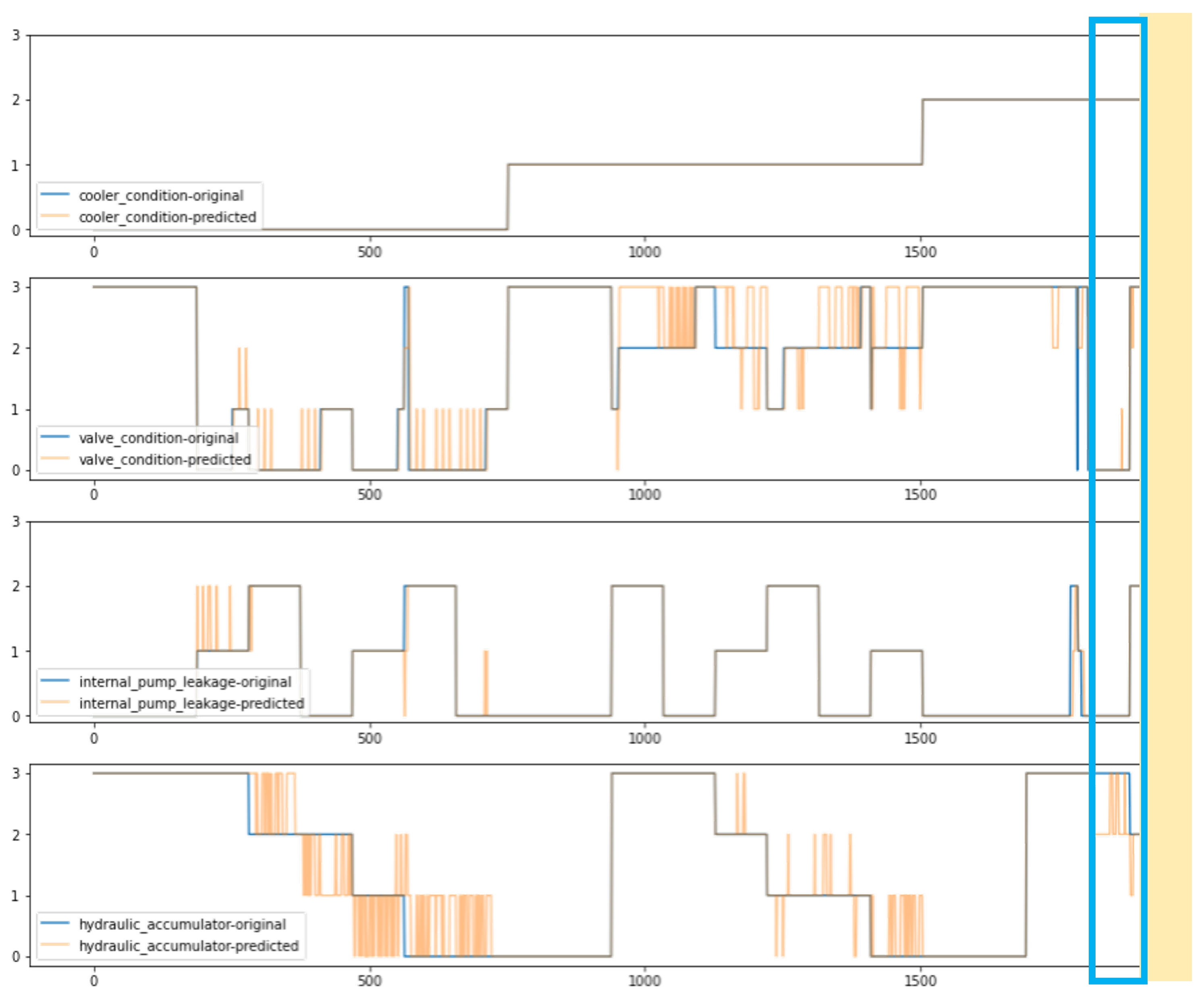
As the working cycle is already segmented into steps, the LSTM model can then predict the faulty cycle before it finishes. As the moving window for prediction reaches the next cycle in Figure 25, deviation occurs in the fourth fault grade; therefore, the system should be stopped.
“Decision space” analysis can be carried out on the output of the model to assess the capability of the model to classify the system operation and the fault grades within each fault class. Since all the introduced model architectures use the same architecture of reserving a separate LSTM branch for predicting the system operation, the results of applying PCA in the decision spaces are similar for all models, as exhibited in Figure 26. It can be seen that although the data points with the “stable” flag are scattered, the “unstable” points are nicely grouped.
In predicting different fault grades with different LSTM architecture, this result in the decision space also reflects the choice in the “Model structure” step. In Figure 27, the first row is the result of PCA on the LSTM layer before the dense layer of Model_0, while the second row is from Model_1, and the third row reflects Model_3 (the structures of these models are mentioned in Figure 16). As Model_0 uses separated LSTM layers to separate the fault levels, four faults have different distributions in the “Decision space”. The first fault is the most well-separated, which suggests a better chance of providing an accurate prediction, while the fourth fault displays the least accurate performance. On the contrary, the results of four fault classifications in the second row were derived from a common single LSTM layer; thus, the faults are forced into a uniform pattern in the decision space.
By comparing the result of applying PCA in the input space and decision space, users can analyze the diagnostic capability of the model. The more clear the boundary between fault grades is, the more possible the model will make a good prediction. It can be seen that the first two components have the most influence on both the input and the decision space and are also the easiest to recognize, while the others can not maintain clear margins between their fault levels. In Model_3, only the first and third faults are derived from a common LSTM layer, while the second and fourth faults are speculated from corresponding separated layers. Therefore, these faults have different distributions in the decision space.
These results from this use case will benefit engineers, developers, and users during model construction and model monitoring. Utilizing the fault-related fact acquired from this explanation, the model can be continuously modified and updated, along with the FDI tool and system performance.

4. Discussion

4.1. The Maturity and Applicability of XAI for ML-Based FDI Solutions

Considering the ML model as the core tool of the FDI solution, a well-designed model can utilize the available data to efficiently and transparently handle fault classification. Although most of the current studies focus on using the XAI concept to develop tools explaining how the ML model works, it can be incorporated during model development to support a user-friendly understanding of model selection and operation. The proposed framework in this study suggested a continuous tuning and improvement loop for model construction and model monitoring with XAI tools.
Regarding the availability of XAI tools, there are several aspects of the conventional FDI problems that were not mentioned in the relevant research. Either the explanation in these aspects was not important for the research purpose or was underestimated by researchers. Most of the current studies focus on using the XAI concept to develop tools explaining how the ML model works and the contributions of each feature. This explanation can be considered “Understandable” information flow. Aspects such as the effect of the learning and validation strategy are unequivocal and attract no interest. Some aspects have many reasons and needs raised in the literature but were not addressed sufficiently, such as “Monitoring and alerting”, “Resource consumption”, and “Architecture evaluation”. This availability is also dependent on the different requirements for FDI tasks in various systems under study. For instance, different frequencies of system components are critical to vibration studies [19]; therefore, the sampling frequency of sensors should be adjustable and require visualization and explanation for later adjustments. However, we think visualization and explanation can be beneficial for every step of the FDI problem since they can inspire further arrangement and modification of the ML model, as shown in the “Reversible” information flow reflected in the above use case. In the proposed framework, the two “Understandable” and “Reversible” information flows work in tandem.
In terms of maturity, the definitions of XAI tools are vast, ranging from proposals to proof-of-concept and to well-standardized tools such as software packages. Built-in visualization (such as a confusion matrix, training, validation accuracy chart, etc.) are indisputably accepted as indispensable tools in ML studies and were deployed in all mentioned studies. There are a few frequently adopted tools (LIME, SHAP), which were used in many cases from many aspects of fault diagnosis to model analysis. Furthermore, several suggested tools are in the early phase, or specifically considered for certain circumstances or intended systems. Despite this imbalance, the rationale behind these tools can be utilized to generalize the common requirement for XAI functions. The fact that explainability gained more interest than robustness in previous studies also raises a concern given both aspects promote reliability and confidence in FDI results, ensuring that the human user is in control of the important decision made by AI [122,123]. From this viewpoint, the authors call for more attention from XAI tool developers in future development, especially special FDI applications, such as in medical or ADAS systems. It is worth mentioning that, since XAI research did not formulate a clear distinction between “explainability” and “interpretability”, with a lack of formalization and quantification of explanations and performance metrics [26], it is challenging to deliver a quantitative measure of completeness and correctness of the explanation map [15], as well as assess the efficiency of “explainability” from different users, and can be a future research direction.
Last but not least, the elaboration of the ML model cannot solely and comprehensively solve the FDI problem. Practical physics- and process-related knowledge from human feedback can be integrated to fine-tune the model [78] and determine a physics-informed network [32]. Other developments on input consistency regularization and fault detection methods should also be updated or refreshed with the XAI concept [13,75]. Furthermore, human intervention is gaining ever-increasing importance in the operation of ML-based intelligence. To this extent, the XAI concept should be accessible not only to educated users and engineers but should also include direct operators. Therefore, different levels of information depth are preferred. The explanation should not only focus on the details of the model operation, but also on the different effects of model constituents on its performance and the intrinsic aspects of physical assets, enabling humans to learn from these facts and adjust the model accordingly.

4.2. Solution Development with MLOps Principles

Researchers in the FDI field have not paid much attention to real-life software development practice, as not all relevant aspects are mentioned in the literature. Most of the reasoning and suggestions came from DevOps, which requires a system control and management mindset to customize. Considering the core principles of MLOps, development activities can be categorized with the proposed framework, which aligns with the PDCA continuous improvement scheme. As the ML-based FDI solution requires updates and evolution depending on data and usage, this approach helps to direct software-development resources efficiently, coping with the investigation, design, and deployment of new features. As following well-defined guidelines allows the traceability and reproducibility of the results [56], more systematic procedures are needed. This comprehensive approach also allows the cooperation of involving stakeholders, where developers and engineers work together on the acquired fact by the ML model from the FDI problem.
By deploying a larger development loop of continuous deployment with human user interference, ethical and responsible ML/AI goals [124] can be achieved. In addition to this human augmentation, bias evaluation is also performed by both humans and the machine itself. With XAI tools ensuring explainability, model life cycles are carefully managed to embrace reproducibility. The cost of developing and choosing an optimal structure and platform for MLOps can be complicated [125], lacking a specific configuration for FDI problems. However, this aspect is out-of-scope, is not mentioned in this study, and requires separate effort in future research.

4.3. Suggestion for a Collaborative Process Monitoring with Human-in-the-Loop Machine Learning

Many efforts have been deployed throughout the ML-relevant literature to improve deep learning in automatic tools that perform process monitoring and FDI tasks independently from human intervention. Most of the FDI solutions mentioned in the literature only deploy XAI tools to explain how the ML model works for a specific system monitoring scenario, without elaborating on how human users can collaborate with the ML model during usage. However, as many recent researchers pointed out, human intelligence can easily solve many cases that are problematic for computer systems [126,127,128,129]; thus, the incorporation of XAI and human users in the development of ML-based FDI solutions should take place in all phases rather than at a later stage of using a one-time built model [65]. A HITL ML pipeline proposed by Chai et al. [130] utilizes human contribution in all steps: data extraction, data integration, data cleaning, data annotation and Iterative labeling, and model training and inference, to alleviate hardness and leverage the usage efficiency during the whole life-cycle of ML-based AI models [131]. From the use case, it can be seen that human users have significantly contributed to the operation and performance of the ML model in the FDI scenarios.
Inspired by the observation–orientation–decision–action (OODA) loop, which emphasized the role of humans to augment the command-and-control decision-making process [132], Figure 28 illustrates a perspective to use the HITL ML for the PHM of industrial systems based on the suggestion from this paper. The three main involved parties are the system, the human, and the machine (ML models). The system includes ongoing processes with possible fault characteristics. The data and status of the system are collected and monitored by the machine. The machine needs supervised development from the human; thus, it can provide the human with explainable models/decisions regarding what it has learned from the system, and start its operation as an FDI tool.
During this continuous operation, the machine supports the human in the process monitoring work; thus, the human can perform necessary system configuration and modification. The collaboration between the machine and the human can be characterized by the OODA loop:
  • Observation: Process the acquired data to obtain knowledge regarding the status of the process and occurring faults within the system.
  • Orientation: Assess the overall situation and operating status of the system.
  • Decision: Consider the initiatives or actions that should be taken given the current situation.
  • Action: Perform the intervention that places an effect on the system.
Depending on certain system management purposes, this collaboration may have different tasks assigned to the machine and the human thanks to the potential capability of the machine. For example, during the fault diagnosis and isolation tasks, the machine can automatically manage the observation–orientation steps, while the other two steps are handled by the human since the analysis of new faults and consideration of actions require human knowledge. Within the process correction and improvement quest, the machine can have more degrees of freedom to suggest possible actions up until the decision step. When it comes to redesigning the process, the machine can also propose a new action plan with the new process or even configure a new process, which is equivalent to the action step.
These interactions between the machine and the human are possible suggestions of how the HITL FDI tool can function with the contribution from the human users to guide the evolution of machine intelligence, especially in situations that are ambiguous for the machine to learn by itself, such as with unstructured and low-quality data sets, trivial redundant data, wrong units, violated integrity constraints, etc. [130]. On the other hand, it makes the FDI solution less vulnerable merely to machine consciousness, while offering humans an off-switch against the future superintelligent AI [133].

5. Conclusions

The XAI concept was not fully matured and thoroughly customized to FDI purposes, especially throughout the development process. A comprehensive and incremental approach should consider applying XAI tools to all stages while integrating new features into a continuous CI/CD pipeline. This research proposed a new approach to building an ML-based FDI solution that utilized XAI and MLOps concepts, with guidelines for organizing relevant development activities. The continuous tuning and improvement process creates a loop between model construction and monitoring, with two directions of information: “Understandable” and “Reversible” explanation. Elaborating on the ML model based on this loop then gathers in-depth knowledge from both objects: the monitored physical system (e.g., the fault characteristics and system performance) and the ML model (e.g., prediction capability and required resources), which benefits both the human and ML model. When placing this loop into the framework of MLOps, the FDI solution is treated as a software product, evolved under incremental updates by a concurrent engineering team. On the other hand, the involvement of human users during operation as a developer is recommended. The combination of these two concepts helps to effectively develop the FDI solution with the shortest time to production while enhancing the trust of human users throughout the elaboration and utilization process.
A use case is carried out on a hydraulic system data set to illustrate possible human intervention during model construction and usage utilizing the XAI concept. The modifications during development are considered based on the explained model operation rules, resulting in a compact, sufficient model while the physical characteristics of the monitored faults are learned. Compared to other high-standardized ETL-based (i.e., extraction, transformation, and loading) commercial software (such as Knime and Pipeline Pilot [134,135]), the proof-of-concept software developed in this study has the possibility to integrate more XAI solutions specialized for FDI problems. Not to mention, endless open-source Python packages can be incorporated, as illustrated during the use case.
This result urges for more adoption of the XAI and MLOps principles in software development with ML models to gain trust in human users on the capability of AI. In general, the OODA interaction between the human, the machine, and the asset facilitates the employment of HITL ML in the industrial asset management field.

Author Contributions

T.-A.T.: Conceptualization, Methodology, Coding, Investigation, Software, Validation, Visualization, Writing—original draft. T.R.: Conceptualization, Methodology, Supervision, Writing—review and editing, Project administration. J.A.: Conceptualization, Methodology, Supervision, Writing—review and editing, Resources. All authors have read and agreed to the published version of the manuscript.

Funding

This work was implemented by the TKP2021-NVA-10 project with support provided by the Ministry of Culture and Innovation of Hungary from the National Research, Development and Innovation Fund, financed under the 2021 Thematic Excellence Programme funding scheme. This research was supported by the National Research, Development, and Innovation Office of Hungary under the project “Research and development of safety-critical brake-by-wire brake systems and intelligent software sensors that can also be used in autonomous vehicles” (project code: 2020-1.1.2-PIACI-KFI-2020-00144).

Data Availability Statement

The datasets were obtained from a public database. The codes and models used to generate the concept demonstration results will be available on request.

Conflicts of Interest

The authors declare no conflicts of interest.

Abbreviations

The following abbreviations are used in this manuscript:
ADASAdvanced Driver-Assistance System
AIArtificial Intelligence
APIApplication Programming Interface
CAMClass Activation Mapping
CBMConditional Based Monitoring
CD/CI   Continuous Deployment/Continuous Integration
CNNConvolutional Neural Networks
DiCEDiverse Counterfactual Explanations
DLDeep Learning
FDIFault Detection and Identification
HITLHuman-in-the-Loop
kNNk-Nearest Neighbors Algorithm
KPIsKey Performance Indicators
LDALinear Discriminant Analysis
LIMELocal Interpretable Model-agnostic Explanations
LSTMLong Short-Term Memory
MLMachine Learning
MLOpsMachine Learning Operations
OODAObservation–Orientation–Decision–Action
OPTICSOrdering Points To Identify the Clustering Structure
PCAPrincipal Component Analysis
PDCAPlan–Do–Check–Act
PHMPrognostic and Health Management
RULRemaining Useful Life
SHAPSHapley Additive exPlanations
SMOTESynthetic Minority Oversampling TEchnique
SVMSupport Vector Machines
t-SNEt-distributed Stochastic Neighbor Embedding
XAIeXplainable Artificial Intelligence
D e n s e _ j The j t h Dense layer
L S T M _ k The k t h LSTM layer
M o d e l _ i The i t h Model
o u t _ h The h t h Output layer

Appendix A. Reasoning from Relevant Literature

Table A1 categorized the suggestions from the literature for each step during “XAI model construction”, along with proposed tools that are tailored to the FDI requirement. As different FDI solutions require different XAI approaches, it is worth mentioning the type of studied systems.
Similarly, relevant aspects and reasoning of the “XAI model monitoring” block are listed in Table A2. Table A3 lists XAI ML-based FDI development phases with associated tasks and corresponding stakeholders.
Table A1. XAI tools in FDI model construction phases.
D.P.AspectReasoning (System & Study)Proposed Tools (Maturity Level)
Data acquisitionSensory data acquisitionShow the monitored system diagram (hydraulic system [38]), Choose the input sensors, identify the Analog input/output (I/O) variables from sensors (i.e., temperature, pressures, power, voltage, etc.) (simulated pick/place system and electric furnace [33], photovoltaic panel [60]) Labeling the fault type from input sensor data (•), system diagram with critical components (••)
Sampling frequencyAdjust the sampling frequency from sensor data (bearing test rig [19])
Signal processingExtract the working status of machines and digital input/output (I/O) variables (sensors and actuators) (simulated pick/place system and electric furnace [33]), visualize the use of different cut-off frequency and digital filters (bearing test rig [19], autonomous underwater vehicles [41])
Data annotationVisualize the rules of identifying and annotating fault conditions (chiller system [18], chemical process [17], bearing test rig [19], air handling unit [54]), defined the first event and variable types (simulated pick/place system and electric furnace [33])Event chart (•), Characteristics table (•), Hierarchical clustering on SHAP values of fault types (••)
Data streamingExplain problems associated with the time-series stream from the programmable logic controller, missing data (simulated pick/place system and electric furnace [33], chemical process [17], autonomous underwater vehicles [41])Data pipeline of collecting and normalizing online data (•)
Input preparationSegmentationDefine sequential cycles (simulated pick/place system and electric furnace  [33]), segmenting the raw signal (motor bearing [23], bearing test rig [19], autonomous underwater vehicles [41], robotic system [136])Segmentation chart (this study) (••)
Feature selectionPrepare feature set from each segmented window (autonomous underwater vehicles [41]), choose the relevant features (motor bearing [23], bearing test rig [19], air handling unit [54]); Combining discrete events and continuous variables (simulated pick/place system and electric furnace [33])Visualized rule for feature set preparation (•), features–faults map (••), SHAP values to analyze the influence of features on each fault instance (•••)
Data transformationTransform the acquired data into frequency domain (rotating electric motor [20], rotating machinery [74], robotic system [136]), transform into spectrograms (motor bearing [23]) or scalogram (robotic system [136]); Scale and prepare the dataset into train and test set (chemical process [17])Frequency revolutions per minute (RPM) and order-RPM heat map (••), spectrograms (•••), scalogram (•••)
Block designVisualize the designed blocks (etching process [55]), the effect of block size and overlap on performance (autonomous underwater vehicles [41]) Control chart in block (••), accuracy chart of different setup (••), block chart to visualize the fault distribution within input data (this study) (••)
Regression considerationSelect the step of time-lag based on the fault detection delay (chemical process [137])Relative relevance plot (••)
Model engineeringModel selectionSelect the model based on prediction accuracy (simulated pick and place system and electric furnace machine [33], bearing test rig [19], photovoltaic panels [60]), or individual case explanation (chiller system [18]), or fault detection rate (FDR) and false alarm rate (FAR) (chemical process [17,75])F1-FDR-FAR score table (••), Contribution maps with SHAP values and reconstruction error (••)
Model structureDeep explanation for the model structure (chiller system [18]) Local Interpretable Model-agnostic Explanations (LIME) to explain the rationale of the decision from the model with triggered performance KPIs (•••)
Learning strategyExplain the learning strategy for each fault, based on fault characteristicsBatch-wise learning (•)
Validation strategyDefine the set or permutation for validation method (rotating machinery [74]), different validation strategiesValidation selection (this study) (••)
Hyper-parameter tuningFine tune the hyper-parameters to achieve the best performance of models (bearing test rig [19], rotating machinery [74], autonomous underwater vehicles [41])
Model executionTraining and Validation accuracyVisualize train and validation accuracy and loss values (bearing test rig [19])Accuracy graph (•••)
Performance evaluationShow the prediction accuracy (photovoltaic panels [60], autonomous underwater vehicles [41])Confusion matrix (•••)
(Hyper)parameter evaluationVisualize the effect of hyper-parameters and parameters (photovoltaic panels [60,66])Parameter score table by meta-heuristic algorithm (••)
Validation effectivenessEstimates the valid duration for each fault prediction, in which the predicted result holds acceptable accuracy
Resource consumptionReport the current time/resource/energy consumption  [60,92] and carbon emission [57,58] to prepare for the model operation Carbon-tracker to track the used energy from model training (••)
Model operationIndividual case predictionExplaining representative individual prediction with fault characteristics and weight (rotating machinery [74], chiller system [18], chemical process [17,75], motor bearing [23], heat recycler [138]), showing a sliding prediction window during operation (air handling unit [54])Fault isolation with reconstruction- and SHAP-based construction (••), SHAP to explain the weight of each feature in prediction of an individual case (•••), LIME to show the effect of variation signals from an individual case on prediction results (•••), sliding prediction window with new incoming sensor data (••)
System performanceExplain the impact of the fault to the monitored system (chiller system [18]), system Remaining Useful Life (RUL) prediction (motor bearing [23], turbofan engines [24], autonomous underwater vehicles [41]), process parameters (etching process [55])Impact analyzer with dialog system (••), RUL chart (••), control chart (••)
FDI performanceShow the model performance with FDI task and preventive ability (turbofan engines [24], chemical process [17]), fault isolation rate (etching process [55], heat recycler [138])Root Mean Square Error and the Scoring function (•), FDR and FAR table (••), isolation rate table (••)
Monitoring and AlertingProvide real-time alert to field personnel (chiller system [18], chemical process [17], air handling unit [54,65], photovoltaic panels [60])Local explanation triggered by Key Performance Indicators (KPIs) (••)
DocumentationStore documentation and reasoning during the model construction.
D.P.: Development phase.
Table A2. XAI tools in FDI model performance monitoring phases.
D.P.AspectReasoning (Study)Proposed Tools (Maturity Level)
Pipeline developmentInput signal attributeAnalyze the contribution of input frequency to the performance (rotating electric motor [20])LIME to elucidate important frequencies and orders in input data of each fault class (•••)
Data augmentationIncrease the number of data in case of data insufficiency or imbalanced data set (air handling unit [65]).Table of fault type and sample size to adjust training data (this study) (••), Synthetic Minority Oversampling TEchnique (SMOTE) to enhance the fault class distribution and eliminate the extreme data unbalance in the training set (•••)
Fault definitionData profiling for each fault type (chiller system [18]), labeling faulty variable with the root cause (etching process [55], bearing test rig [19]), show the frequency distribution of associated sensor signals (hydraulic system [38]) determine the beginning of fault (rotating machinery [74])Operating condition chart (•), Fault table with fault rules (•), waterfall envelop spectrum (••), frequency distribution table (••)
Input data managementStores the current data set, and visualizes the changes in input data and a short history of faults (air handling unit [54])Moving window of fault frequency (this study) (••)
Input sufficiencyInput space analysisAnalyze the effect of the input data set: data set size, the train/test split, number of faulty samples (simulated pick/place system & electric furnace [33]); data distribution (chemical process [17], motor bearing [23]), data imbalance (rotating electric motor [20], photovoltaic panel [66]), detect anomaly input sample (rotating machinery [74])K-means clustering on training data (••), LIME to analyze the local data points in the input space (•••), observation table (••)
Learned featuresThe feature characteristics of fault can be determined based on the knowledge from the previous sprint (bearing test rig [19], rotating machinery [74], air handling unit [65])Provide quantitative explanations of each feature to the fault prediction with SHAP (•••), signal samples of fault types (••)
Regression sensitivityConsider the effect of different values of regressive time stepBox-plot of model accuracy over regressive time step (this study) (••)
Resource consumptionConsider the computational power for performing FDI tasks with the trained model on computers or embedded systems (simulated pick/place system and electric furnace [33])
Structure efficiencyArchitecture evaluationEvaluate the compactness and utilization of the architecture; The appropriateness of the output for prediction purpose (turbofan engines [24])
Layer activationEvaluate the activation map of layers (rotating electric motor [20])Class Activation Mapping (CAM) variants (•••), Layer-wise Relevance Propagation (LRP) variants (•••)
Cell activationEvaluate the utilization of unit in each LSTM cellPrincipal Component Analysis (PCA) on cells in one layer (this study) (••)
Fault learning rateEvaluate how much data is required to learn each fault type
Decision rulesFault diagnosisVisualized fault characteristics and behaviors (photovoltaic panels [60]), visualized the causal interaction of process system (etching process [55])Characteristic curve of fault (••), fault causal network (••)
Feature contributionExplain the relevance of timed-events and continuous variables features (simulated pick/place system & electric furnace [33]); the contribution of features (turbofan engines [24], chemical process [17], bearing test rig [19], rotating electric motor [20], rotating machinery [74], chiller system [18]) SHAP to rate the contribution of features an individual case (•••), LIME to define the threshold of each feature on an individual case (•••), Ablation study by Pycaret library [139] (•••), Local-Depth-based Isolation Forest Feature Importance (Local-DIFFI) (•••)
Decision criteriaExplain the decision range of each feature for an observation (photovoltaic panel [66]), the difference between faulty to normal operating condition (chemical process [75]), root cause analysis between different fault (rotating machinery [74])Anchors (•••), Diverse Counterfactual Explanations (DiCE) (•••), root cause feature ranking (••)
Decision trajectory trackingExplaining the inflation of monitoring index for both latent and construction space (chemical process [17]), Track the activation trajectory of fault cases (chemical process [140])Average gradient against scaled deviation (••), PCA trajectory of LSTM layer (this study) (••)
Diagnostic capabilityDecision space analysisAnalyze the capability of the model based on the distinguishability of faults in construction space (chemical process [17]), on the output layer (turbofan engines [24]), or based on the PCA on activation values of latent space (vinyl acetate simulated process [112]).Hierarchical clustering on SHAP-based contribution (••), PCA on LSTM layer of fault branch (this study) (••)
Robustness analysisVisualize the effect of signal-fluctuation faults (e.g., sensor drift and simultaneous faults) (chemical process [17]), false alarm (photovoltaic panels [60]), explanation stability and consistency (photovoltaic panels [66])Explanation chart with fault deviation (••), box plot of SHAP/DiCE values (••)
Uncertainty quantificationProvide the uncertainty estimated for prediction results (turbofan engines [24])Rolling standard deviation plot of Health Index (••)
Abnormal analysisAnalyze the diagnostic capability against rare and abnormal events (chemical process [17], rotating machinery [74]), abnormal working conditions (photovoltaic panels [60]) and hypothetical observation (photovoltaic panels [66])F1-FDR-FAR score table of faults (••), accuracy and error charts (••), DiCE (•••)
D.P.: Development phase.
Table A3. MLOp blocks and phases for XAI ML-based FDI development.
D.P.Step(Main) S.H.Reasoning (Study)
Model planningPrior process understanding(BS, HU); DSSketch the model requirements based on prior knowledge and business requirement [30,54,56].
Physics-informed feedback(DS; HU); DEImprove the model with the learned physics-informed feedback [17,87].
Improvement idea(HU); BSIgnite the next development/refinement loop via Kaizen activities [86];
Requirement analysis(HU; DS;) MLADefine a use case for the next development/refinement [81]
Exploratory Data Analysis(DA)Analyze the data availability before the next development cycle [81]
Initial modeling(DE; MLA); SEPrepare an initial model to assess model feasibility [81]
Model constructionAPI/Development environment(SE); MLAEstablish the API and development environment [27,60,81]
Cloud/fog/edge integration(DOE); SEFDI task execution can be implemented on cloud, fog, or edge services [33,60]
Continuous Deployment/Continuous Integration pipeline (CD/CI) and platform(DOE); SEEstablish an automated ML workflow [30,83,92]
Compression and scaling(SE; DOE); MLABuild a compact model which is suitable for scaling [30]
Model
monitoring
Model metrics and logs(DS); DE; HUManage the model registry with associated performance metrics and logs [27,30,60,81].
Pipeline monitoring(DOE); SE; DEMonitoring the performance of the established pipeline [92]
Ground truth monitoring(DE); HU; DOEManage and track the ground truth of faults after each model development [19,24,94]
Drift monitoring(DE); DOECope with the drift of incoming data from original Data/Model/Concept [27,81,95,141]
Decay monitoring(DOE; DE); DSEstablish a procedure to detect and alert the model decay during production [56,81]
Continuous training(DOE); DEDevelop a matured MLOps system by retraining [96]
Trust-based optimization(HU); DOEFine tune the model operation based on modeling the human trust [98]
Data feedback loop(DOE); MLACreate an informed network with knowledge integration workflow [78]
Model
refinement
Alarm reset and Acceptance(DOE), SE, HURefine the model by human request [84], or analyze the alarm acceptance rate [18,60]
Self-assessment(DOE), SE, HUUse random feedback from human users to update the next model revolution [84,94]
Fault analysis and Update(DA); HU; BSAnalyze the fault based on newly achieved knowledge, and update the fault characteristics
Random data generation(DS); MLAEnrich data for self-validation, or solve data imbalance problems [99]
Trust management(DOE; SE;) HU; DSManage the required information and individual preference for trust establishment [101,102]
Request and Self-triggering(HU), BSSelf-execute [30], request for human clarification [94], adjustment [84], or retrain with predefined threshold [81]
Model life cycle managementRepository management(DOE); SEManage the data and source code throughout model revolutions [27,30,81]
New model introduction(DOE; SE)Introduce new model incremental updates or features into the staging/production environment [27,81].
New model integration and testing(SE); DE; MLAGradually updating new model update after each testing trials [30,81]
Performance comparison(DOE; DS); DE; HUCompare performance between newly deployed model with the previous versions [30,81]
Approval and Production update(DOE); SE; BSApprove the new update and launch production phase [81]
Model troubleshooting(SE); DOEReset the model into previous version when necessary [81]
Production model governanceVersioning(DOE); SERecord the previous models were deployed in production [81].
Lineage tracking and Audit trials(DOE); MLA; SEPerform the regular audit trial and collect audit results during development and usage [81].
Data security(SE); DEResolve security issues and grant control access to stakeholders [44,81]
Data privacy(DE); SEValidate the conformity with privacy rights and regulations (i.e., General Data Protection Regulation (GDPA) and California Consumer Privacy Act (CCPA)) [81].
Packaging(SE); DOE; DEWarp up the necessary codes and platform for each model [81].
Reporting(SE); BSProvide requested documentation and information for model usage [81]
D.P.: Development phase; S.H.: stakeholders. BS: business stakeholder; DS: data Scientist; DE: data engineer; DOE: DevOps engineer; HU: human users; SE: software Engineer; MLA: machine learning architect.

References

  1. Haddad, D.; Wang, L.; Kallel, A.Y.; Amara, N.E.B.; Kanoun, O. Multi-sensor-based method for multiple hard faults identification in complex wired networks. In Proceedings of the 2022 IEEE 9th International Conference on Computational Intelligence and Virtual Environments for Measurement Systems and Applications (CIVEMSA), Chemnitz, Germany, 15–17 June 2022; pp. 1–5. [Google Scholar]
  2. Yu, W.; Wu, M.; Huang, B.; Lu, C. A generalized probabilistic monitoring model with both random and sequential data. Automatica 2022, 144, 110468. [Google Scholar] [CrossRef]
  3. Jia, F.; Lei, Y.; Guo, L.; Lin, J.; Xing, S. A neural network constructed by deep learning technique and its application to intelligent fault diagnosis of machines. Neurocomputing 2018, 272, 619–628. [Google Scholar] [CrossRef]
  4. Su, K.; Liu, J.; Xiong, H. Hierarchical diagnosis of bearing faults using branch convolutional neural network considering noise interference and variable working conditions. Knowl.-Based Syst. 2021, 230, 107386. [Google Scholar] [CrossRef]
  5. Gupta, M.; Wadhvani, R.; Rasool, A. A real-time adaptive model for bearing fault classification and remaining useful life estimation using deep neural network. Knowl.-Based Syst. 2023, 259, 110070. [Google Scholar] [CrossRef]
  6. Khan, S.; Yairi, T. A review on the application of deep learning in system health management. Mech. Syst. Signal Process. 2018, 107, 241–265. [Google Scholar] [CrossRef]
  7. Yu, W.; Zhao, C.; Huang, B.; Xie, M. An unsupervised fault detection and diagnosis with distribution dissimilarity and lasso penalty. IEEE Trans. Control Syst. Technol. 2023, 32, 767–779. [Google Scholar] [CrossRef]
  8. Qin, S.J. Survey on data-driven industrial process monitoring and diagnosis. Annu. Rev. Control 2012, 36, 220–234. [Google Scholar] [CrossRef]
  9. Lei, Y.; Yang, B.; Jiang, X.; Jia, F.; Li, N.; Nandi, A.K. Applications of machine learning to machine fault diagnosis: A review and roadmap. Mech. Syst. Signal Process. 2020, 138, 106587. [Google Scholar] [CrossRef]
  10. Castelvecchi, D. Can we open the black box of AI? Nat. News 2016, 538, 20. [Google Scholar] [CrossRef]
  11. Lipton, Z.C. The mythos of model interpretability: In machine learning, the concept of interpretability is both important and slippery. Queue 2018, 16, 31–57. [Google Scholar] [CrossRef]
  12. Tian, Y.; Zhang, Y. A comprehensive survey on regularization strategies in machine learning. Inf. Fusion 2022, 80, 146–166. [Google Scholar] [CrossRef]
  13. Sevillano-García, I.; Luengo, J.; Herrera, F. SHIELD: A regularization technique for eXplainable Artificial Intelligence. arXiv 2024, arXiv:2404.02611. [Google Scholar]
  14. Arrieta, A.B.; Díaz-Rodríguez, N.; Del Ser, J.; Bennetot, A.; Tabik, S.; Barbado, A.; García, S.; Gil-López, S.; Molina, D.; Benjamins, R.; et al. Explainable Artificial Intelligence (XAI): Concepts, taxonomies, opportunities and challenges toward responsible AI. Inf. Fusion 2020, 58, 82–115. [Google Scholar] [CrossRef]
  15. Das, A.; Rad, P. Opportunities and challenges in explainable artificial intelligence (xai): A survey. arXiv 2020, arXiv:2006.11371. [Google Scholar]
  16. Ahmed, I.; Jeon, G.; Piccialli, F. From artificial intelligence to explainable artificial intelligence in industry 4.0: A survey on what, how, and where. IEEE Trans. Ind. Inform. 2022, 18, 5031–5042. [Google Scholar] [CrossRef]
  17. Jang, K.; Pilario, K.E.S.; Lee, N.; Moon, I.; Na, J. Explainable Artificial Intelligence for Fault Diagnosis of Industrial Processes. IEEE Trans. Ind. Inform. 2023; in press. [Google Scholar]
  18. Srinivasan, S.; Arjunan, P.; Jin, B.; Sangiovanni-Vincentelli, A.L.; Sultan, Z.; Poolla, K. Explainable AI for chiller fault-detection systems: Gaining human trust. Computer 2021, 54, 60–68. [Google Scholar] [CrossRef]
  19. Brusa, E.; Cibrario, L.; Delprete, C.; Di Maggio, L.G. Explainable AI for Machine Fault Diagnosis: Understanding Features’ Contribution in Machine Learning Models for Industrial Condition Monitoring. Appl. Sci. 2023, 13, 2038. [Google Scholar] [CrossRef]
  20. Mey, O.; Neufeld, D. Explainable AI Algorithms for Vibration Data-Based Fault Detection: Use Case-Adadpted Methods and Critical Evaluation. Sensors 2022, 22, 9037. [Google Scholar] [CrossRef]
  21. Hamilton, D.; Pacheco, R.; Myers, B.; Peltzer, B. kNN vs. SVM: A Comparison of Algorithms. Fire-Contin.-Prep. Future Wildland Fire Missoula USA 2018, 78, 95–109. [Google Scholar]
  22. Hasan, M.J.; Sohaib, M.; Kim, J.M. An explainable ai-based fault diagnosis model for bearings. Sensors 2021, 21, 4070. [Google Scholar] [CrossRef]
  23. Sanakkayala, D.C.; Varadarajan, V.; Kumar, N.; Soni, G.; Kamat, P.; Kumar, S.; Patil, S.; Kotecha, K. Explainable AI for Bearing Fault Prognosis Using Deep Learning Techniques. Micromachines 2022, 13, 1471. [Google Scholar] [CrossRef] [PubMed]
  24. Nor, A.K.M. Failure Prognostic of Turbofan Engines with Uncertainty Quantification and Explainable AI (XIA). Turk. J. Comput. Math. Educ. (TURCOMAT) 2021, 12, 3494–3504. [Google Scholar] [CrossRef]
  25. Nor, A.K.B.M.; Pedapait, S.R.; Muhammad, M. Explainable ai (xai) for phm of industrial asset: A state-of-the-art, prisma-compliant systematic review. arXiv 2021, arXiv:2107.03869. [Google Scholar]
  26. Saeed, W.; Omlin, C. Explainable AI (XAI): A systematic meta-survey of current challenges and future opportunities. Knowl.-Based Syst. 2023, 263, 110273. [Google Scholar] [CrossRef]
  27. Ruf, P.; Madan, M.; Reich, C.; Ould-Abdeslam, D. Demystifying mlops and presenting a recipe for the selection of open-source tools. Appl. Sci. 2021, 11, 8861. [Google Scholar] [CrossRef]
  28. Alla, S.; Adari, S.K.; Alla, S.; Adari, S.K. What is mlops? In Beginning MLOps with MLFlow: Deploy Models in AWS SageMaker, Google Cloud, and Microsoft Azure; Apress: New York, NY, USA, 2021; pp. 79–124. [Google Scholar]
  29. Lwakatare, L.E.; Kuvaja, P.; Oivo, M. Relationship of devops to agile, lean and continuous deployment: A multivocal literature review study. In Proceedings of the Product-Focused Software Process Improvement: 17th International Conference, PROFES 2016, Trondheim, Norway, 22–24 November 2016; Proceedings 17. Springer: Berlin/Heidelberg, Germany, 2016; pp. 399–415. [Google Scholar]
  30. Karamitsos, I.; Albarhami, S.; Apostolopoulos, C. Applying DevOps practices of continuous automation for machine learning. Information 2020, 11, 363. [Google Scholar] [CrossRef]
  31. Tamburri, D.A. Sustainable mlops: Trends and challenges. In Proceedings of the 2020 22nd International Symposium on Symbolic and Numeric Algorithms for Scientific Computing (SYNASC), Timisoara, Romania, 1–4 September 2020; pp. 17–23. [Google Scholar]
  32. Chen, Y.; Rao, M.; Feng, K.; Zuo, M.J. Physics-Informed LSTM hyperparameters selection for gearbox fault detection. Mech. Syst. Signal Process. 2022, 171, 108907. [Google Scholar] [CrossRef]
  33. Leite, D.; Martins, A., Jr.; Rativa, D.; De Oliveira, J.F.; Maciel, A.M. An Automated Machine Learning Approach for Real-Time Fault Detection and Diagnosis. Sensors 2022, 22, 6138. [Google Scholar] [CrossRef]
  34. Zöller, M.A.; Titov, W.; Schlegel, T.; Huber, M.F. XAutoML: A Visual Analytics Tool for Establishing Trust in Automated Machine Learning. arXiv 2022, arXiv:2202.11954. [Google Scholar]
  35. Helwig, N.; Pignanelli, E.; Schütze, A. Condition monitoring of a complex hydraulic system using multivariate statistics. In Proceedings of the 2015 IEEE International Instrumentation and Measurement Technology Conference (I2MTC) Proceedings, Pisa, Italy, 11–14 May 2015; pp. 210–215. [Google Scholar]
  36. Schneider, T.; Helwig, N.; Schütze, A. Automatic feature extraction and selection for classification of cyclical time series data. tm-Tech. Mess. 2017, 84, 198–206. [Google Scholar] [CrossRef]
  37. Huang, K.; Wu, S.; Li, F.; Yang, C.; Gui, W. Fault diagnosis of hydraulic systems based on deep learning model with multirate data samples. IEEE Trans. Neural Netw. Learn. Syst. 2021, 33, 6789–6801. [Google Scholar] [CrossRef] [PubMed]
  38. Keleko, A.T.; Kamsu-Foguem, B.; Ngouna, R.H.; Tongne, A. Health condition monitoring of a complex hydraulic system using Deep Neural Network and DeepSHAP explainable XAI. Adv. Eng. Softw. 2023, 175, 103339. [Google Scholar] [CrossRef]
  39. Goelles, T.; Schlager, B.; Muckenhuber, S. Fault detection, isolation, identification and recovery (fdiir) methods for automotive perception sensors including a detailed literature survey for lidar. Sensors 2020, 20, 3662. [Google Scholar] [CrossRef] [PubMed]
  40. Keipour, A.; Mousaei, M.; Scherer, S. Automatic real-time anomaly detection for autonomous aerial vehicles. In Proceedings of the 2019 International Conference on Robotics and Automation (ICRA), Montreal, QC, Canada, 20–24 May 2019; pp. 5679–5685. [Google Scholar]
  41. Das, D.B.; Birant, D. GASEL: Genetic algorithm-supported ensemble learning for fault detection in autonomous underwater vehicles. Ocean. Eng. 2023, 272, 113844. [Google Scholar]
  42. Ribeiro, M.T.; Singh, S.; Guestrin, C. “Why should i trust you?” Explaining the predictions of any classifier. In Proceedings of the 22nd ACM SIGKDD International Conference on Knowledge Discovery and Data Mining, New York, NY, USA, 13–17 August 2016; pp. 1135–1144. [Google Scholar]
  43. Love, P.E.; Fang, W.; Matthews, J.; Porter, S.; Luo, H.; Ding, L. Explainable artificial intelligence (XAI): Precepts, models, and opportunities for research in construction. Adv. Eng. Inform. 2023, 57, 102024. [Google Scholar] [CrossRef]
  44. Shahbazi, Z.; Byun, Y.C. Integration of blockchain, IoT and machine learning for multistage quality control and enhancing security in smart manufacturing. Sensors 2021, 21, 1467. [Google Scholar] [CrossRef]
  45. Molnar, C. Interpretable Machine Learning, 2nd ed.; Lulu.com: Morrisville, NC, USA, 2022. [Google Scholar]
  46. Kravchenko, T.; Bogdanova, T.; Shevgunov, T. Ranking requirements using MoSCoW methodology in practice. In Proceedings of the Computer Science On-Line Conference, Virtual, 26–30 April 2022; Springer: Berlin/Heidelberg, Germany, 2022; pp. 188–199. [Google Scholar]
  47. Paleyes, A.; Urma, R.G.; Lawrence, N.D. Challenges in deploying machine learning: A survey of case studies. Acm Comput. Surv. 2022, 55, 1–29. [Google Scholar] [CrossRef]
  48. Zhang, Y.; Patel, S. Agile model-driven development in practice. IEEE Softw. 2010, 28, 84–91. [Google Scholar] [CrossRef]
  49. Jäger, D.; Gümmer, V. PythonDAQ–A Python based measurement data acquisition and processing software. J. Phys. Conf. Ser. 2023, 2511, 012016. [Google Scholar] [CrossRef]
  50. Weber, S. PyMoDAQ: An open-source Python-based software for modular data acquisition. Rev. Sci. Instrum. 2021, 92, 045104. [Google Scholar] [CrossRef]
  51. Martins, S.A.M. PYDAQ: Data Acquisition and Experimental Analysis with Python. J. Open Source Softw. 2023, 8, 5662. [Google Scholar] [CrossRef]
  52. Mozafari, B.; Sarkar, P.; Franklin, M.; Jordan, M.; Madden, S. Scaling up crowd-sourcing to very large datasets: A case for active learning. Proc. Vldb Endow. 2014, 8, 125–136. [Google Scholar] [CrossRef]
  53. Ehrenberg, H.R.; Shin, J.; Ratner, A.J.; Fries, J.A.; Ré, C. Data programming with ddlite: Putting humans in a different part of the loop. In Proceedings of the Workshop on Human-In-the-Loop Data Analytics, New York, NY, USA, 26 June–1 July 2016; pp. 1–6. [Google Scholar]
  54. Meas, M.; Machlev, R.; Kose, A.; Tepljakov, A.; Loo, L.; Levron, Y.; Petlenkov, E.; Belikov, J. Explainability and Transparency of Classifiers for Air-Handling Unit Faults Using Explainable Artificial Intelligence (XAI). Sensors 2022, 22, 6338. [Google Scholar] [CrossRef] [PubMed]
  55. Yang, W.T.; Reis, M.S.; Borodin, V.; Juge, M.; Roussy, A. An interpretable unsupervised Bayesian network model for fault detection and diagnosis. Control Eng. Pract. 2022, 127, 105304. [Google Scholar] [CrossRef]
  56. Testi, M.; Ballabio, M.; Frontoni, E.; Iannello, G.; Moccia, S.; Soda, P.; Vessio, G. MLOps: A Taxonomy and a Methodology. IEEE Access 2022, 10, 63606–63618. [Google Scholar] [CrossRef]
  57. Budennyy, S.A.; Lazarev, V.D.; Zakharenko, N.N.; Korovin, A.N.; Plosskaya, O.; Dimitrov, D.V.; Akhripkin, V.; Pavlov, I.; Oseledets, I.V.; Barsola, I.S.; et al. Eco2ai: Carbon emissions tracking of machine learning models as the first step towards sustainable ai. Dokl. Math. 2022, 106 (Suppl. S1), S118–S128. [Google Scholar] [CrossRef]
  58. Anthony, L.F.W.; Kanding, B.; Selvan, R. Carbontracker: Tracking and predicting the carbon footprint of training deep learning models. arXiv 2020, arXiv:2007.03051. [Google Scholar]
  59. Géron, A. Hands-on Machine Learning with Scikit-Learn, Keras, and TensorFlow; O’Reilly Media, Inc.: Sebastopol, CA, USA, 2022. [Google Scholar]
  60. Sairam, S.; Seshadhri, S.; Marafioti, G.; Srinivasan, S.; Mathisen, G.; Bekiroglu, K. Edge-based Explainable Fault Detection Systems for photovoltaic panels on edge nodes. Renew. Energy 2022, 185, 1425–1440. [Google Scholar] [CrossRef]
  61. Bouza, L.; Bugeau, A.; Lannelongue, L. How to estimate carbon footprint when training deep learning models? A guide and review. Environ. Res. Commun. 2023, 5, 115014. [Google Scholar] [CrossRef]
  62. Al-Aomar, R. A methodology for determining Process and system-level manufacturing performance metrics. Sae Trans. 2002, 1043–1056. [Google Scholar]
  63. Frank, S.M.; Lin, G.; Jin, X.; Singla, R.; Farthing, A.; Zhang, L.; Granderson, J. Metrics and Methods to Assess Building Fault Detection and Diagnosis Tools; Technical Report; National Renewable Energy Lab. (NREL): Golden, CO, USA, 2019. [Google Scholar]
  64. Zhu, T.; Lin, Y.; Liu, Y. Synthetic minority oversampling technique for multiclass imbalance problems. Pattern Recognit. 2017, 72, 327–340. [Google Scholar] [CrossRef]
  65. Belikov, J.; Meas, M.; Machlev, R.; Kose, A.; Tepljakov, A.; Loo, L.; Petlenkov, E.; Levron, Y. Explainable AI based fault detection and diagnosis system for air handling units. In Proceedings of the International Conference on Informatics in Control, Automation and Robotics, Lisbon, Portugal, 14–16 July 2022; pp. 14–16. [Google Scholar]
  66. Utama, C.; Meske, C.; Schneider, J.; Schlatmann, R.; Ulbrich, C. Explainable artificial intelligence for photovoltaic fault detection: A comparison of instruments. Sol. Energy 2023, 249, 139–151. [Google Scholar] [CrossRef]
  67. He, M.; Li, B.; Sun, S. A Survey of Class Activation Mapping for the Interpretability of Convolution Neural Networks. In Signal and Information Processing, Networking and Computers: Proceedings of the 10th International Conference on Signal and Information Processing, Networking and Computers (ICSINC), Xi’Ning, China, July 2022; Springer: Berlin/Heidelberg, Germany, 2023; pp. 399–407. [Google Scholar]
  68. Montavon, G.; Binder, A.; Lapuschkin, S.; Samek, W.; Müller, K.R. Layer-wise relevance propagation: An overview. In Explainable AI: Interpreting, Explaining and Visualizing Deep Learning; Springer: Berlin/Heidelberg, Germany, 2019; pp. 193–209. [Google Scholar]
  69. Van den Broeck, G.; Lykov, A.; Schleich, M.; Suciu, D. On the tractability of SHAP explanations. J. Artif. Intell. Res. 2022, 74, 851–886. [Google Scholar] [CrossRef]
  70. Laves, M.H.; Ihler, S.; Ortmaier, T. Uncertainty Quantification in Computer-Aided Diagnosis: Make Your Model say “I don’t know” for Ambiguous Cases. arXiv 2019, arXiv:1908.00792. [Google Scholar]
  71. Shafaei, S.; Kugele, S.; Osman, M.H.; Knoll, A. Uncertainty in machine learning: A safety perspective on autonomous driving. In Proceedings of the Computer Safety, Reliability, and Security: SAFECOMP 2018 Workshops, ASSURE, DECSoS, SASSUR, STRIVE, and WAISE, Västerås, Sweden, 18 September 2018; Proceedings 37. Springer: Berlin/Heidelberg, Germany, 2018; pp. 458–464. [Google Scholar]
  72. Chen, N.C.; Drouhard, M.; Kocielnik, R.; Suh, J.; Aragon, C.R. Using machine learning to support qualitative coding in social science: Shifting the focus to ambiguity. Acm Trans. Interact. Intell. Syst. (TiiS) 2018, 8, 1–20. [Google Scholar] [CrossRef]
  73. Munro, R.; Monarch, R. Human-in-the-Loop Machine Learning: Active Learning and Annotation for Human-Centered AI; Simon and Schuster: New York, NY, USA, 2021. [Google Scholar]
  74. Brito, L.C.; Susto, G.A.; Brito, J.N.; Duarte, M.A. An explainable artificial intelligence approach for unsupervised fault detection and diagnosis in rotating machinery. Mech. Syst. Signal Process. 2022, 163, 108105. [Google Scholar] [CrossRef]
  75. Harinarayan, R.R.A.; Shalinie, S.M. XFDDC: EXplainable Fault Detection Diagnosis and Correction framework for chemical process systems. Process. Saf. Environ. Prot. 2022, 165, 463–474. [Google Scholar] [CrossRef]
  76. Ghosh, A.; Nachman, B.; Whiteson, D. Uncertainty-aware machine learning for high energy physics. Phys. Rev. D 2021, 104, 056026. [Google Scholar] [CrossRef]
  77. Li, W.; Li, H.; Gu, S.; Chen, T. Process fault diagnosis with model-and knowledge-based approaches: Advances and opportunities. Control Eng. Pract. 2020, 105, 104637. [Google Scholar] [CrossRef]
  78. Kim, S.W.; Kim, I.; Lee, J.; Lee, S. Knowledge Integration into deep learning in dynamical systems: An overview and taxonomy. J. Mech. Sci. Technol. 2021, 35, 1331–1342. [Google Scholar] [CrossRef]
  79. Sovrano, F.; Vitali, F. An objective metric for explainable AI: How and why to estimate the degree of explainability. Knowl.-Based Syst. 2023, 278, 110866. [Google Scholar] [CrossRef]
  80. Breck, E.; Cai, S.; Nielsen, E.; Salib, M.; Sculley, D. The ML test score: A rubric for ML production readiness and technical debt reduction. In Proceedings of the 2017 IEEE International Conference on Big Data (Big Data), Boston, MA, USA, 11–14 December 2017; pp. 1123–1132. [Google Scholar]
  81. Larysa, V.; Anja, K.; Isabel, B.; Alexander, K.; Michael, P. MLOps Principles. 2022. Available online: https://ml-ops.org/content/mlops-principles (accessed on 11 September 2024).
  82. Treveil, M.; Omont, N.; Stenac, C.; Lefevre, K.; Phan, D.; Zentici, J.; Lavoillotte, A.; Miyazaki, M.; Heidmann, L. Introducing MLOps; O’Reilly Media: Sebastopol, CA, USA, 2020. [Google Scholar]
  83. Kreuzberger, D.; Kühl, N.; Hirschl, S. Machine learning operations (mlops): Overview, definition, and architecture. IEEE Access 2023, 11, 31866–31879. [Google Scholar] [CrossRef]
  84. Abonyi, J.; Babuška, R.; Szeifert, F. Fuzzy expert system for supervision in adaptive control. Ifac Proc. Vol. 2000, 33, 241–246. [Google Scholar] [CrossRef]
  85. Shearer, C. The CRISP-DM model: The new blueprint for data mining. J. Data Warehous. 2000, 5, 13–22. [Google Scholar]
  86. Awad, M.; Shanshal, Y.A. Utilizing Kaizen process and DFSS methodology for new product development. Int. J. Qual. Reliab. Manag. 2017, 34, 378–394. [Google Scholar] [CrossRef]
  87. Karpatne, A.; Watkins, W.; Read, J.; Kumar, V. How can physics inform deep learning methods in scientific problems?: Recent progress and future prospects. In Proceedings of the 31st Conference on Neural Information Processing Systems (NeurIPS), Long Beach, CA, USA, 4–9 December 2017; pp. 1–5. [Google Scholar]
  88. Cuomo, S.; Di Cola, V.S.; Giampaolo, F.; Rozza, G.; Raissi, M.; Piccialli, F. Scientific machine learning through physics–informed neural networks: Where we are and what’s next. J. Sci. Comput. 2022, 92, 88. [Google Scholar] [CrossRef]
  89. Arachchi, S.; Perera, I. Continuous integration and continuous delivery pipeline automation for agile software project management. In Proceedings of the 2018 Moratuwa Engineering Research Conference (MERCon), Moratuwa, Sri Lanka, 30 May–1 June 2018; pp. 156–161. [Google Scholar]
  90. Neely, S.; Stolt, S. Continuous delivery? easy! just change everything (well, maybe it is not that easy). In Proceedings of the 2013 Agile Conference, Nashville, TN, USA, 5–9 August 2013; pp. 121–128. [Google Scholar]
  91. Humble, J.; Farley, D. Continuous Delivery: Reliable Software Releases through Build, Test, and Deployment Automation; Pearson Education: London, UK, 2010. [Google Scholar]
  92. Zhou, Y.; Yu, Y.; Ding, B. Towards mlops: A case study of ml pipeline platform. In Proceedings of the 2020 International Conference on Artificial Intelligence and Computer Engineering (ICAICE), Beijing, China, 23–25 October 2020; pp. 494–500. [Google Scholar]
  93. Pathania, N. Learning Continuous Integration with Jenkins: A Beginner’s Guide to Implementing Continuous Integration and Continuous Delivery Using Jenkins 2; Packt Publishing Ltd.: Birmingham, UK, 2017. [Google Scholar]
  94. Ding, K.; Li, J.; Liu, H. Interactive anomaly detection on attributed networks. In Proceedings of the Twelfth ACM International Conference on Web Search and Data Mining, New York, NY, USA, 11–15 February 2019; pp. 357–365. [Google Scholar]
  95. Baier, L.; Kühl, N.; Satzger, G. How to Cope with Change? Preserving Validity of Predictive Services over Time. In Proceedings of the Hawaii International Conference on System Sciences (HICSS-52), Wailea, HI, USA, 8–11 January 2019; University of Hawai’i at Manoa/AIS. pp. 1085–1094. [Google Scholar]
  96. Symeonidis, G.; Nerantzis, E.; Kazakis, A.; Papakostas, G.A. MLOps-definitions, tools and challenges. In Proceedings of the 2022 IEEE 12th Annual Computing and Communication Workshop and Conference (CCWC), Las Vegas, NV, USA, 26–29 January 2022; pp. 453–460. [Google Scholar]
  97. Gujjar, J.P.; Kumar, V.N. Demystifying mlops for continuous delivery of the product. Asian J. Adv. Res. 2022, 5, 19–23. [Google Scholar]
  98. Akash, K.; McMahon, G.; Reid, T.; Jain, N. Human trust-based feedback control: Dynamically varying automation transparency to optimize human-machine interactions. IEEE Control Syst. Mag. 2020, 40, 98–116. [Google Scholar] [CrossRef]
  99. Fan, Y.; Cui, X.; Han, H.; Lu, H. Chiller fault detection and diagnosis by knowledge transfer based on adaptive imbalanced processing. Sci. Technol. Built Environ. 2020, 26, 1082–1099. [Google Scholar] [CrossRef]
  100. Liao, Q.V.; Varshney, K.R. Human-centered explainable ai (xai): From algorithms to user experiences. arXiv 2021, arXiv:2110.10790. [Google Scholar]
  101. Drozdal, J.; Weisz, J.; Wang, D.; Dass, G.; Yao, B.; Zhao, C.; Muller, M.; Ju, L.; Su, H. Trust in AutoML: Exploring information needs for establishing trust in automated machine learning systems. In Proceedings of the 25th International Conference on Intelligent User Interfaces, Greenville, SC, USA, 18–21 March 2020; pp. 297–307. [Google Scholar]
  102. Ozsoy, M.G.; Polat, F. Trust based recommendation systems. In Proceedings of the 2013 IEEE/ACM International Conference on Advances in Social Networks Analysis and Mining, New York, NY, USA, 25–28 August 2013; pp. 1267–1274. [Google Scholar]
  103. Katayama, H. Legend and future horizon of lean concept and technology. Procedia Manuf. 2017, 11, 1093–1101. [Google Scholar] [CrossRef]
  104. Lima, A.; Rossi, L.; Musolesi, M. Coding together at scale: GitHub as a collaborative social network. In Proceedings of the International AAAI Conference on Web and Social Media, Ann Arbor, MI, USA, 1–4 June 2014; Volume 8, pp. 295–304. [Google Scholar]
  105. Directorate-General for Communications Networks, Content and Technology, European Commission. European Approach to Artificial Intelligence. 2023. Available online: https://digital-strategy.ec.europa.eu/en/policies/european-approach-artificial-intelligence (accessed on 11 September 2024).
  106. Burns, B.; Beda, J.; Hightower, K.; Evenson, L. Kubernetes: Up and Running; O’Reilly Media, Inc.: Sebastopol, CA, USA, 2022. [Google Scholar]
  107. Butcher, M.; Farina, M.; Dolitsky, J. Learning Helm; O’Reilly Media: Sebastopol, CA, USA, 2021. [Google Scholar]
  108. Helwig, N.; Pignanelli, E.; Schtze, A. Condition monitoring of hydraulic systems Data Set. Uci Mach. Learn. Repos. 2018, 46, 66121. [Google Scholar] [CrossRef]
  109. Helwig, N. Detecting and Compensating Sensor Faults in a Hydraulic Condition Monitoring System. In Proceedings of the SENSOR 2015—17th International Conference on Sensors and Measurement Technology, Nuremberg, Germany, 19–21 May 2015. oral presentation D8.1. [Google Scholar]
  110. Malhotra, P.; Vig, L.; Shroff, G.; Agarwal, P. Long Short Term Memory Networks for Anomaly Detection in Time Series. In Proceedings of the ESANN, Bruges, Belgium, 22–24 April 2015; Volume 2015, p. 89. [Google Scholar]
  111. Lu, W.; Li, Y.; Cheng, Y.; Meng, D.; Liang, B.; Zhou, P. Early fault detection approach with deep architectures. IEEE Trans. Instrum. Meas. 2018, 67, 1679–1689. [Google Scholar] [CrossRef]
  112. Dorgo, G.; Pigler, P.; Abonyi, J. Understanding the importance of process alarms based on the analysis of deep recurrent neural networks trained for fault isolation. J. Chemom. 2018, 32, e3006. [Google Scholar] [CrossRef]
  113. Truong, C.; Oudre, L.; Vayatis, N. Selective review of offline change point detection methods. Signal Process. 2020, 167, 107299. [Google Scholar] [CrossRef]
  114. Law, S.M. STUMPY: A Powerful and Scalable Python Library for Time Series Data Mining. J. Open Source Softw. 2019, 4, 1504. [Google Scholar] [CrossRef]
  115. Zhao, K.; Wulder, M.A.; Hu, T.; Bright, R.; Wu, Q.; Qin, H.; Li, Y.; Toman, E.; Mallick, B.; Zhang, X.; et al. Detecting change-point, trend, and seasonality in satellite time series data to track abrupt changes and nonlinear dynamics: A Bayesian ensemble algorithm. Remote. Sens. Environ. 2019, 232, 111181. [Google Scholar] [CrossRef]
  116. Schwartz, M.; Pataky, T.C.; Donnelly, C.J. seg1d: A Python package for Automated segmentation of one-dimensional (1D) data. J. Open Source Softw. 2020, 5, 2404. [Google Scholar] [CrossRef]
  117. Truong, C.; Oudre, L.; Vayatis, N. ruptures: Change point detection in Python. arXiv 2018, arXiv:1801.00826. [Google Scholar]
  118. Pedregosa, F.; Varoquaux, G.; Gramfort, A.; Michel, V.; Thirion, B.; Grisel, O.; Blondel, M.; Prettenhofer, P.; Weiss, R.; Dubourg, V.; et al. Scikit-learn: Machine Learning in Python. J. Mach. Learn. Res. 2011, 12, 2825–2830. [Google Scholar]
  119. Roberts, D.R.; Bahn, V.; Ciuti, S.; Boyce, M.S.; Elith, J.; Guillera-Arroita, G.; Hauenstein, S.; Lahoz-Monfort, J.J.; Schröder, B.; Thuiller, W.; et al. Cross-validation strategies for data with temporal, spatial, hierarchical, or phylogenetic structure. Ecography 2017, 40, 913–929. [Google Scholar] [CrossRef]
  120. Anowar, F.; Sadaoui, S.; Selim, B. Conceptual and empirical comparison of dimensionality reduction algorithms (pca, kpca, lda, mds, svd, lle, isomap, le, ica, t-sne). Comput. Sci. Rev. 2021, 40, 100378. [Google Scholar] [CrossRef]
  121. Chollet, F. Keras. 2015. Available online: https://github.com/fchollet/keras (accessed on 11 September 2024).
  122. Holzinger, A. The next frontier: AI we can really trust. In Proceedings of the Joint European Conference on Machine Learning and Knowledge Discovery in Databases, Virtual, 13–17 September 2021; Springer: Berlin/Heidelberg, Germany, 2021; pp. 427–440. [Google Scholar]
  123. Holzinger, A.; Dehmer, M.; Emmert-Streib, F.; Cucchiara, R.; Augenstein, I.; Del Ser, J.; Samek, W.; Jurisica, I.; Díaz-Rodríguez, N. Information fusion as an integrative cross-cutting enabler to achieve robust, explainable, and trustworthy medical artificial intelligence. Inf. Fusion 2022, 79, 263–278. [Google Scholar] [CrossRef]
  124. Saxena, D.; Lamest, M.; Bansal, V. Responsible machine learning for ethical artificial intelligence in business and industry. In Handbook of Research on Applied Data Science and Artificial Intelligence in Business and Industry; IGI Global: Hershey, PA, USA, 2021; pp. 639–653. [Google Scholar]
  125. Faubel, L.; Schmid, K. A Systematic Analysis of MLOps Features and Platforms. WiPiEC J.-Work. Prog. Embed. Comput. J. 2024, 10, 97–104. [Google Scholar]
  126. Holzinger, A. Interactive machine learning for health informatics: When do we need the human-in-the-loop? Brain Inform. 2016, 3, 119–131. [Google Scholar] [CrossRef] [PubMed]
  127. Holzinger, A.; Plass, M.; Holzinger, K.; Crişan, G.C.; Pintea, C.M.; Palade, V. Towards interactive Machine Learning (iML): Applying ant colony algorithms to solve the traveling salesman problem with the human-in-the-loop approach. In Proceedings of the Availability, Reliability, and Security in Information Systems: IFIP WG 8.4, 8.9, TC 5 International Cross-Domain Conference, CD-ARES 2016, and Workshop on Privacy Aware Machine Learning for Health Data Science, PAML 2016, Salzburg, Austria, 31 August–2 September 2016; Proceedings. Springer: Berlin/Heidelberg, Germany, 2016; pp. 81–95. [Google Scholar]
  128. Ramesh, P.V.; Subramaniam, T.; Ray, P.; Devadas, A.K.; Ramesh, S.V.; Ansar, S.M.; Ramesh, M.K.; Rajasekaran, R.; Parthasarathi, S. Utilizing human intelligence in artificial intelligence for detecting glaucomatous fundus images using human-in-the-loop machine learning. Indian J. Ophthalmol. 2022, 70, 1131. [Google Scholar] [CrossRef]
  129. Yang, Y.; Kandogan, E.; Li, Y.; Sen, P.; Lasecki, W.S. A Study on Interaction in Human-in-the-Loop Machine Learning for Text Analytics. In Proceedings of the IUI Workshops, Los Angeles, CA, USA, 19–20 March 2019; pp. 1–7. [Google Scholar]
  130. Chai, C.; Li, G. Human-in-the-loop Techniques in Machine Learning. IEEE Data Eng. Bull. 2020, 43, 37–52. [Google Scholar]
  131. Wu, X.; Xiao, L.; Sun, Y.; Zhang, J.; Ma, T.; He, L. A survey of human-in-the-loop for machine learning. Future Gener. Comput. Syst. 2022, 135, 364–381. [Google Scholar] [CrossRef]
  132. Johnson, J. Automating the OODA loop in the age of intelligent machines: Reaffirming the role of humans in command-and-control decision-making in the digital age. Def. Stud. 2022, 23, 43–67. [Google Scholar] [CrossRef]
  133. Brundage, M. Taking superintelligence seriously: Superintelligence: Paths, dangers, strategies by Nick Bostrom (Oxford University Press, 2014). Futures 2015, 72, 32–35. [Google Scholar] [CrossRef]
  134. Berthold, M.R.; Cebron, N.; Dill, F.; Gabriel, T.R.; Kötter, T.; Meinl, T.; Ohl, P.; Thiel, K.; Wiswedel, B. KNIME-the Konstanz information miner: Version 2.0 and beyond. ACM SIGKDD Explor. Newsl. 2009, 11, 26–31. [Google Scholar] [CrossRef]
  135. Warr, W.A. Scientific workflow systems: Pipeline Pilot and KNIME. J. Comput.-Aided Mol. Des. 2012, 26, 801–804. [Google Scholar] [CrossRef] [PubMed]
  136. Raouf, I.; Kumar, P.; Lee, H.; Kim, H.S. Transfer Learning-Based Intelligent Fault Detection Approach for the Industrial Robotic System. Mathematics 2023, 11, 945. [Google Scholar] [CrossRef]
  137. Agarwal, P.; Tamer, M.; Budman, H. Explainability: Relevance based dynamic deep learning algorithm for fault detection and diagnosis in chemical processes. Comput. Chem. Eng. 2021, 154, 107467. [Google Scholar] [CrossRef]
  138. Madhikermi, M.; Malhi, A.K.; Främling, K. Explainable artificial intelligence based heat recycler fault detection in air handling unit. In Proceedings of the Explainable, Transparent Autonomous Agents and Multi-Agent Systems: First International Workshop, EXTRAAMAS 2019, Montreal, QC, Canada, 13–14 May 2019; Revised Selected Papers 1. Springer: Berlin/Heidelberg, Germany, 2019; pp. 110–125. [Google Scholar]
  139. Ali, M. PyCaret: An Open Source, Low-Code Machine Learning Library in Python. PyCaret Version 1.0. 2020. Available online: https://github.com/pycaret/pycaret (accessed on 11 September 2024).
  140. Bhakte, A.; Pakkiriswamy, V.; Srinivasan, R. An explainable artificial intelligence based approach for interpretation of fault classification results from deep neural networks. Chem. Eng. Sci. 2022, 250, 117373. [Google Scholar] [CrossRef]
  141. Baier, L.; Schlör, T.; Schöffer, J.; Kühl, N. Detecting concept drift with neural network model uncertainty. arXiv 2021, arXiv:2107.01873. [Google Scholar]
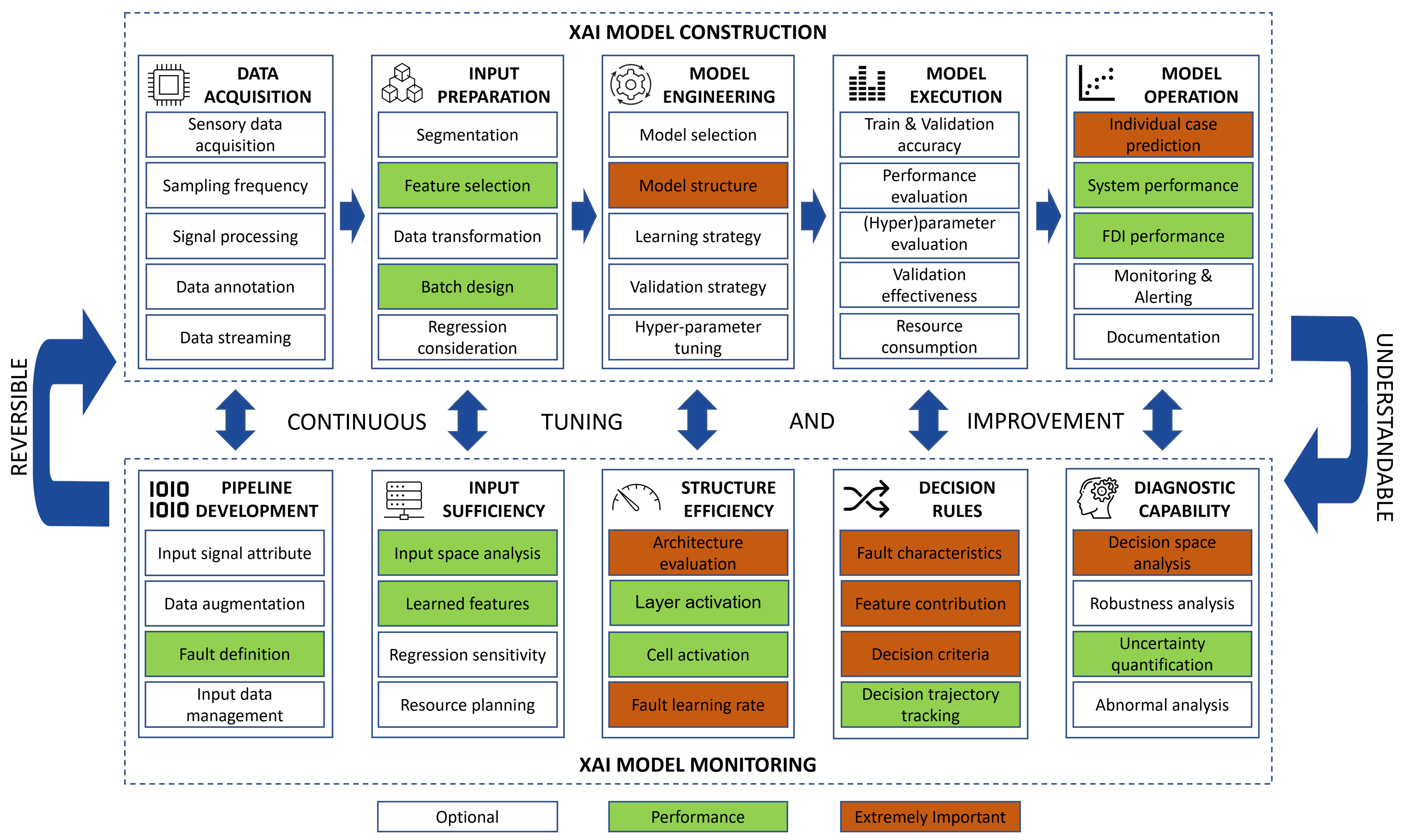
Figure 1. The proposed framework for the XAI-integrated development of ML-based FDI solutions.
Computers 13 00252 g001
Figure 2. The proposed MLOps framework for developing an XAI-integrated ML-based FDI solution. In the middle the PDCA is the plan–do–check–act cycle.
Computers 13 00252 g002
Figure 3. The hydraulic system with the main working circuit (a) and cooling and filtration circuit (b). The four targeted system elements for FDI are marked with red squares: (1) cooler, (2) valve, (3) pump, and (4) accumulators. Source: Helwig et al. [35].
Computers 13 00252 g003
Figure 4. The proportion of fault grades within four critical components (left) with optimal working states shown in green color and close-to-failure states in red. The proportion of system fault status within the stable/unstable operating mode is shown on the stacked bar chart on the (right).
Computers 13 00252 g004
Figure 5. The LSTM architecture for FDI solution. Adapted from [112].
Computers 13 00252 g005
Figure 6. Activation from a single LSTM cell during the FDI task. Adapted from [112].
Computers 13 00252 g006
Figure 7. The FDI solution with multiple fault classes and multiple fault grades.
Computers 13 00252 g007
Figure 8. Two typical operating modes when there is no fault in any critical component, which yield a stable (upper) and not-yet-stable (lower) system status, with the 17 sensor signals from different cycles within these modes. Although there was no fault, variance can be observed in the signals from PS4, PS5, PS6, and all the temperature sensors when the system was not stable (lower).
Computers 13 00252 g008
Figure 9. The moving window of “Input data management”, which represents the frequency of new appearing fault cases. Except for three cases with an unusually high frequency, the other cases appeared around ten times throughout the input data.
Computers 13 00252 g009
Figure 10. The segmentation step can be performed and visualized with different available tools: (a) Rbeast, (b) stumpy, (c) seg1d methods, and (e) rupture are chosen with (d) the raw signal example and (f) the visualization of segmentation on the other sensor signal of interest, i.e., CP sensor. Each package has a different built-in visualization. At first, a predefined number of change points (dashed lines) are detected, then the margins of these points (dotted lines) are detected backward and forward.
Computers 13 00252 g010
Figure 11. The data block design with the visualization of the fault grades of the cooler condition (upper left), pump condition (upper right), accumulator condition (lower left), and valve condition (lower right). With this visualization, the engineers or users can determine if the division of the data block and the separation are appropriate to capture the variation within each fault grade.
Computers 13 00252 g011
Figure 12. Input space analysis with PCA applied to 1020 original features (left); the 19th and 24th features have the highest loadings on the first principal component (both positive and negative, respectively), while the 874th feature highly influences the second. After choosing a set of two first principal components after PCA and 114 components of highest loadings on these two components, t-SNE is applied to distinguish system status (right).
Computers 13 00252 g012
Figure 13. System status in the input space analysis after applying t-SNE with 1500 perplexity and 0.05 divergence. The status of the first and second elements heavily influence the input space. When both these components are functioning normally (i.e., [ 10 X X ] statuses), the data points are distributed in the middle line of the ball-like space. When only the second element is in a faulty state (i.e., [ 01 X X ] statuses), the data points are shifted to the right of the “ball”. When only the first element is in a faulty state (i.e., [ 10 X X ] statuses), the data points switch to the left. When both these components have problems (i.e., [ 11 X X ] statuses), the data points will be scattered throughout the “ball”.
Computers 13 00252 g013
Figure 14. Once a good distribution of the cooler fault class is achieved with t-SNE (left), OPTICS is applied to cluster the data points of each fault grade (right), where three detected clusters are visualized with three different colors. Outliers or abnormal data appear as unclustered points or noise. The epsilon distance is visualized for better adjustment. As a disadvantage of density-based clustering, it can be observed that the points in the borders of the clusters are classified into noise or wrong clusters, while the noise points that are close to each other (at the lower part) are identified as a separate cluster.
Computers 13 00252 g014
Figure 15. The learned LSTM weight from Model_0 for each fault type (left) ((a): cooler, (b): valve, (c): pump, (d): accumulator) and the effect of LSTM length on the prediction accuracy of the third fault (e).
Computers 13 00252 g015
Figure 16. The evolution of model structure: Model_0: separated fault branch. Model_1: shared branch. Model_2: reinforced branch for the second and fourth faults simultaneously. Model_3: reinforced branch for the second and fourth faults separately. Note: All these models use a separate LSTM branch to recognize system status, which is not shown here for the sake of simplicity.
Computers 13 00252 g016
Figure 17. The different validation strategies with adjustable parameters (upper): (from left to right) k-fold, time series split, and block split. The first and second train-test data division with k-fold as the chosen validation strategy (lower).
Computers 13 00252 g017
Figure 18. LSTM layer activation with the first fault branch (top) from Model_3. (from left to right) The first LSTM layer (LSTM_0) has 12 cells, and the second LSTM layer (LSTM_11) has one cell. The last Dense_1 layer indicates the fault grades. LSTM layer activation of the fourth fault branch (bottom) from LSTM_4, LSTM_41, and Dense_4.
Computers 13 00252 g018
Figure 19. LSTM cell activation with different behaviors: (a) remain constant, (b) reverse, (c) remain neutral, and (d) change from neutral.
Computers 13 00252 g019
Figure 20. The train and validation accuracy of predicting component faults (in percentage) from models with different architectures. Noticeably, Model_1 has low and varied values of training accuracy for the second and fourth faults. Adding separate LSTM layers for the 2nd and 4th fault types helps to improve performance.
Computers 13 00252 g020
Figure 21. The confusion matrix from Model_2. It can be seen that the system operation is well recognized, while the prediction of system faults still needs improvement. The first three faults have a good classification result, while the fourth has the worst one with misclassified results between the first and second fault grades.
Computers 13 00252 g021
Figure 22. PCA result on the 1st, 4th, 8th, 10th, and 12th cells on the LSTM_0 layer in the first fault branch of Model_2. It can be seen that the PCA algorithm tried to separate three levels of this fault type into different clusters throughout the cells. The 8th cell seems to yield better clusters than the others. Moving forward with the next cells does not improve the result.
Computers 13 00252 g022
Figure 23. PCA result on the 1st, 4th, 8th, 10th, and 12th cells on the LSTM_2 and the last LSTM_21 in the second fault branch of Model_3. The LSTM_2 layer of this model is designed to learn both the characteristics of the second and fourth faults. Even at the last cell of this layer, the different levels of the second fault were not well clustered. Only on the last LSTM_21 layer did the model learn to separate four levels of this fault successfully, as the PCA result showed a decent recognizable result.
Computers 13 00252 g023
Figure 24. The PCA results on the weight of the cells in the last LSTM layer for the first fault (left) and the third fault (right) from Model_3. This model has separate branches to learn each of these fault types. It can be seen that for the first fault, the learned results from the 4th, 5th, and 8th cell of the LSTM layer contribute a similar positive effect on the fault classification on the first principal component as the 10th and 12th cell have on the second principal component. The third fault was learned by the other branch differently, with the 4th and 5th cells having effects in different directions on the first principal component.
Computers 13 00252 g024
Figure 25. The moving window for prediction (the blue box) with the next cycle indicated in yellow. From top to bottom: the predicted fault grades for the first to the fourth faults.
Computers 13 00252 g025
Figure 26. Decision space analysis of system operation with PCA results on the last LSTM layers (similar for all models).
Computers 13 00252 g026
Figure 27. Decision space analysis of four fault types with PCA results on the last LSTM layers of Model_0 (top), Model_1 (middle), and Model_3 (bottom).
Computers 13 00252 g027
Figure 28. Human-in-the-loop machine learning based on an OODA loop between the system, the human, and the machine.
Computers 13 00252 g028
Table 1. Characteristics of input signals.
SensorPhysical MeaningUnitSampling RateData PointsRange [Min; Max Value]Mean (Standard Deviation)Skewness
PS1Pressurebar100 Hz6000 [ 133.13 ;   191.92 ] 160.49 ( 16.13 ) 0.98
PS2Pressurebar100 Hz6000 [ 0.0 ;   167.77 ] 109.38 ( 48.1 ) 1.68
PS3Pressurebar100 Hz6000 [ 0.0 ;   18.828 ] 1.75 ( 0.93 ) 0.4
PS4Pressurebar100 Hz6000 [ 0.0 ;   10.266 ] 2.6 ( 4.3 ) 1.14
PS5Pressurebar100 Hz6000 [ 8.318 ;   10.041 ] 9.16 ( 0.58 ) 0.15
PS6Pressurebar100 Hz6000 [ 8.268 ;   9.91 ] 9.08 ( 0.55 ) 0.15
EPS1Motor powerW100 Hz6000 [ 2097.8 ;   2995.2 ] 2495.51 ( 218.22 ) 0.81
FS1Volume flowL/min10 Hz600 [ 0.0 ;   20.479 ] 6.2 ( 3.21 ) 0.92
FS2Volume flowL/min10 Hz600 [ 8.764 ;   10.453 ] 9.65 ( 0.45 ) 0.24
TS1Temperature°C1 Hz60 [ 34.984 ;   58.207 ] 45.42 ( 7.99 ) 0.11
TS2Temperature°C1 Hz60 [ 40.707 ;   62.176 ] 50.37 ( 7.4 ) 0.09
TS3Temperature°C1 Hz60 [ 38.145 ;   59.539 ] 47.66 ( 7.45 ) 0.12
TS4Temperature°C1 Hz60 [ 30.355 ;   53.145 ] 40.74 ( 8.11 ) 0.06
VS1Vibrationmm/s1 Hz60 [ 0.483 ;   2.546 ] 0.61 ( 0.08 ) 2.56
CECooling efficiency (virtual)%1 Hz60 [ 0.0 ;   100.6 ] 55.29 ( 25.64 ) 1.49
CPCooling power (virtual)kW1 Hz60 [ 17.042 ;   48.777 ] 31.3 ( 11.58 ) 0.46
SEEfficiency factor%1 Hz60 [ 1.016 ;   2.909 ] 1.81 ( 0.28 ) 0.3
Disclaimer/Publisher’s Note: The statements, opinions and data contained in all publications are solely those of the individual author(s) and contributor(s) and not of MDPI and/or the editor(s). MDPI and/or the editor(s) disclaim responsibility for any injury to people or property resulting from any ideas, methods, instructions or products referred to in the content.