
GFLASSO-LR: Logistic Regression with Generalized Fused LASSO for Gene Selection in High-Dimensional Cancer Classification

 , , , and
Abstract
1. Introduction
- Introduced an improved approach for dimension reduction and important gene selection in cancer research using DNA microarray technology.
- Integrated gene selection with classifier training into a single process, enhancing the efficiency of identifying cancerous tumors.
- Formulated gene selection as a logistic regression problem with a generalized Fused LASSO (GFLASSO) regularizer, incorporating dual penalties to balance gene relevance and redundancy.
- Utilized a sub-gradient algorithm for optimization, demonstrating the algorithm’s objective function is convex, Lipschitzian, and possesses a global minimum, meeting necessary convergence conditions.
- Showed that the GFLASSO-LR method significantly improves cancer classification from high-dimensional microarray data, yielding compact and highly performant gene subsets.
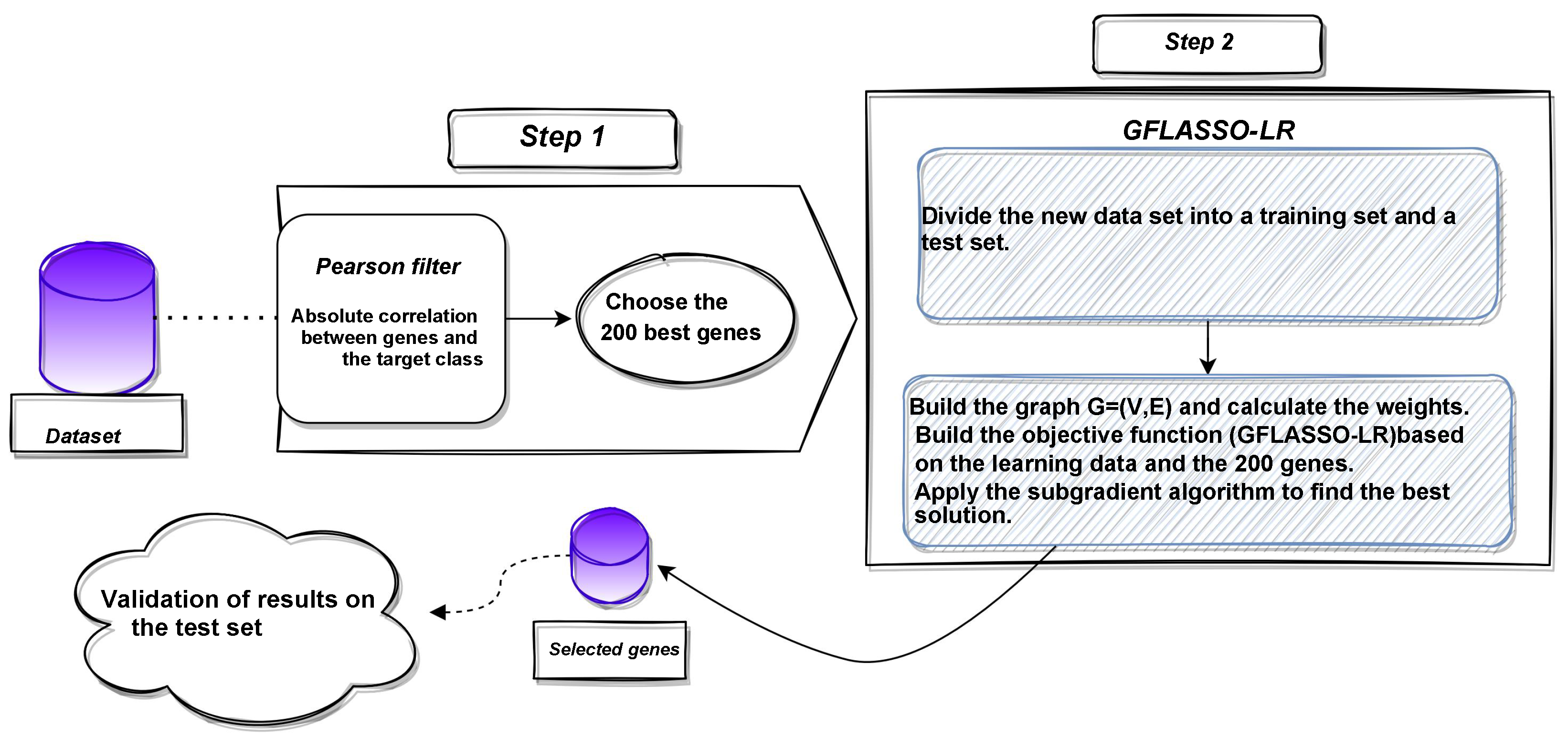
2. Methods
2.1. Preliminaries
- , or simply for any vector of , it was noted that
- is the usual scalar product.
2.2. Sub-Gradient Method
- Let , then is a non-empty, convex, bounded set.
- Assuming differentiability of f at , we have and
- Suppose is a convex set in , and let be convex functions with for . If , then the subdifferential sum rule is expressed as follows:
2.2.1. Subgradient Algorithm
- Suppose for all . Then there exists a positive constant such that
- Suppose thatThen, we have convergence as , and
- Suppose the generated sequence in (5) satisfies
2.2.2. Generalized Fused LASSO
2.2.3. Structure of the Proposed Approach
2.3. Sub-Gradient for Estimating
- It is convex.
- It admits a global minimum.
- It is Lipschitz.
2.3.1. Characteristics and Convexity Analysis of the GFLASSO Penalty Function
- 1.
- The convexity of :First, there isLet us show that g is convex on :
- The function is convex; it is a linear function on .
- The function is convex for all i in , so is convex for all i in . (It is the composition of an increasing function convex on and a convex function on ).
The function g is therefore convex on , being the sum of convex functions. On the other hand, the function is convex as the sum of convex functions.Next, we show that the function is convex.Indeed, let with . The function is convex. This is because , defined in Example (2), is composed of an affine function and another convex one, with . Then the function is convex as it is a sum of convex functions.Finally, we can deduce that the function is convex as it is a sum of convex functions. - 2.
- The existence of a global minimum of :We recall that a real-valued function is coercive if .We haveandwith for all i in .Additionally, we have. SoHence,Let us examine the expression for . Given that the function g is positive on and in (10) is strictly positive, it follows thatBased on the latest inequality, we can deduce that is a coercive function. Additionally, is continuous, so it attains a a global minimum at least once (see appendix in reference [70]).
- 3.
- The function is ℓ-Lipschitz on :We only have one condition left to establish to show that the sub-gradient algorithm converges to a global minimum of ; it is to prove that is ℓ-Lipschitzian on , i.e., find a positive ℓ such thatNote in passing that the Lipschitz constant ℓ depends on the choice of the norm on . Since all norms are equivalent on , whether a function is Lipschitz or not does not depend on the chosen norm.Let us start by showing that the function g is Lipschitz. We first haveThe function g is of class on . Find the partial derivatives of g:Let . We haveTherefore,Let . Then we haveAs we are working on the finite dimensional normed vector space , there then exists some positive such thatWe can notice that the real does not depend on ; more precisely it only depends on the training set. So we getSo g is a -Lipschitz function on by the mean value inequality.In the following, we will prove that the function is Lipschitz.Let . We haveSimilarly, since the weights ,Thereby,andBy norm equivalence, we can deduce that there are some positive and such thatFinally, it suffices to take to deduce that is ℓ-lipschitzian on .
2.3.2. Sub-Gradient Algorithm
3. Experiments and Results
3.1. Datasets
3.2. Settings
| Algorithm 1: Subgradient algorithm to minimize . |
|
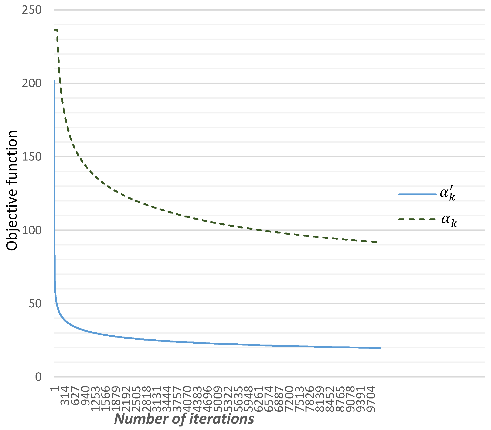
3.2.1. Choice of
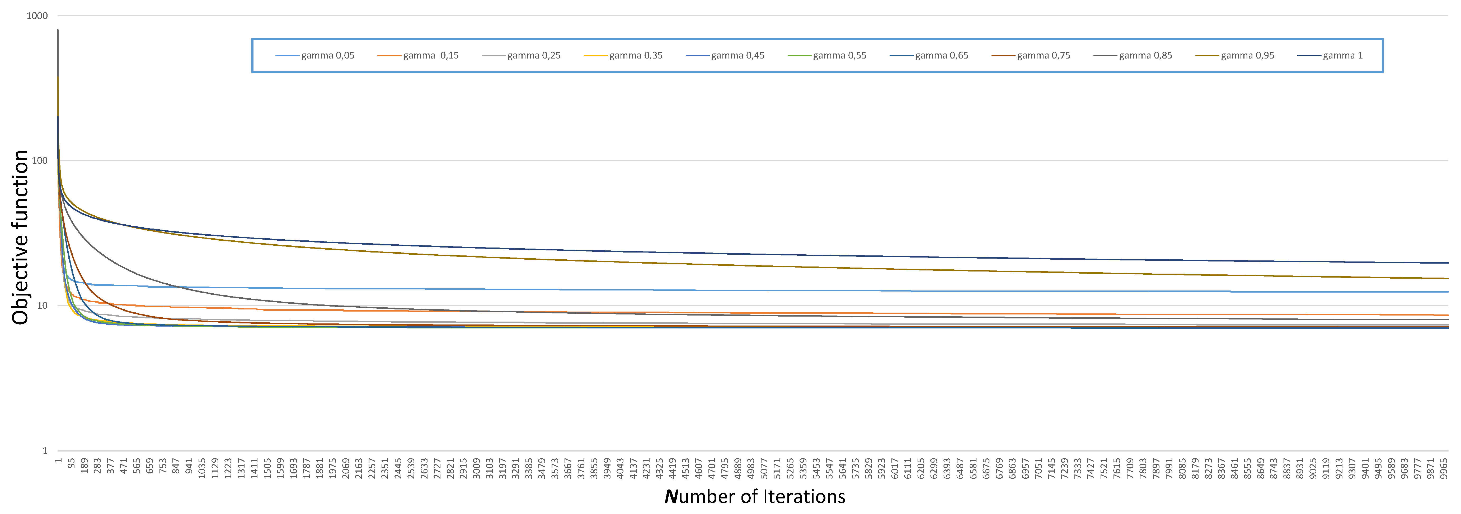
3.2.2. Choice of and
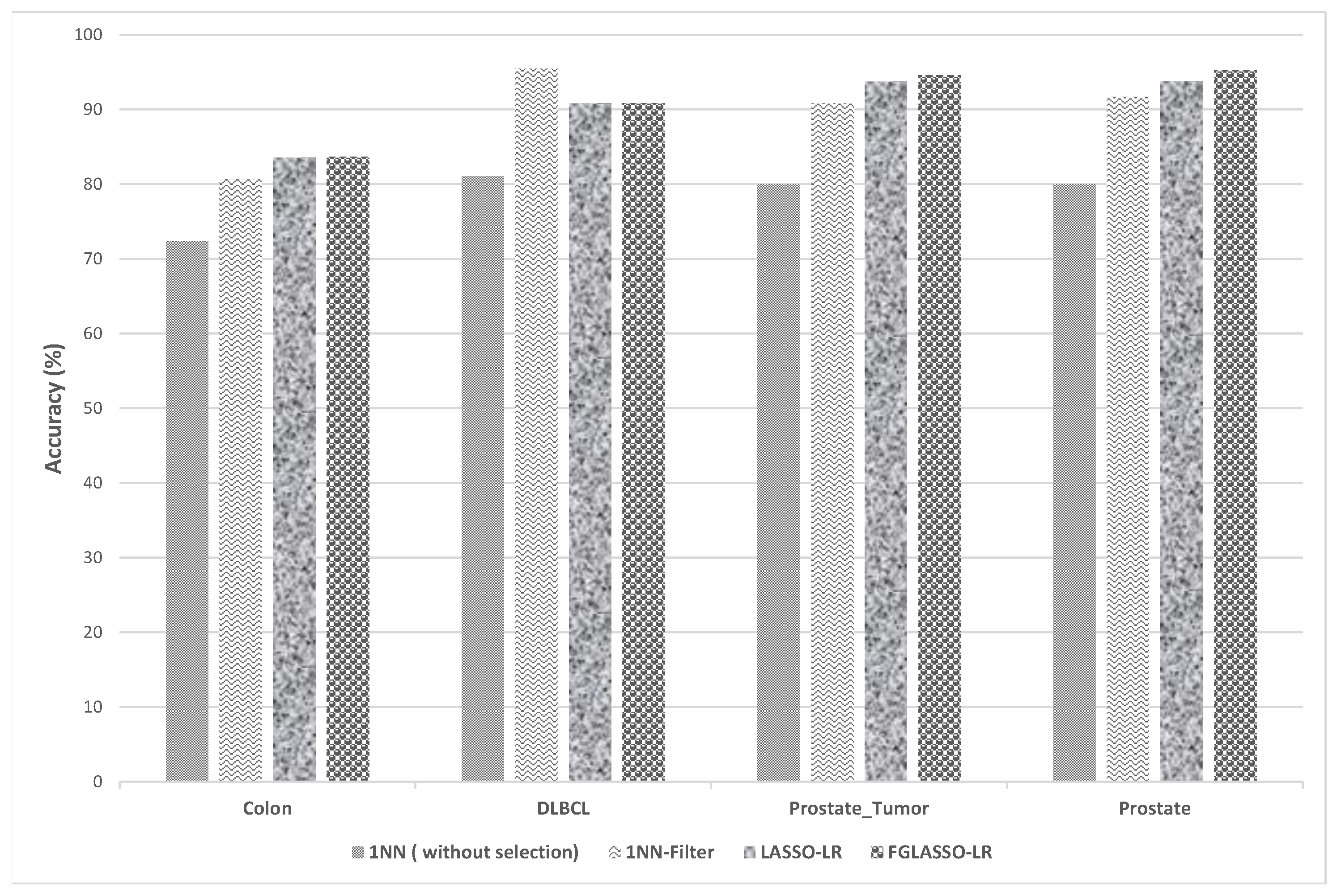
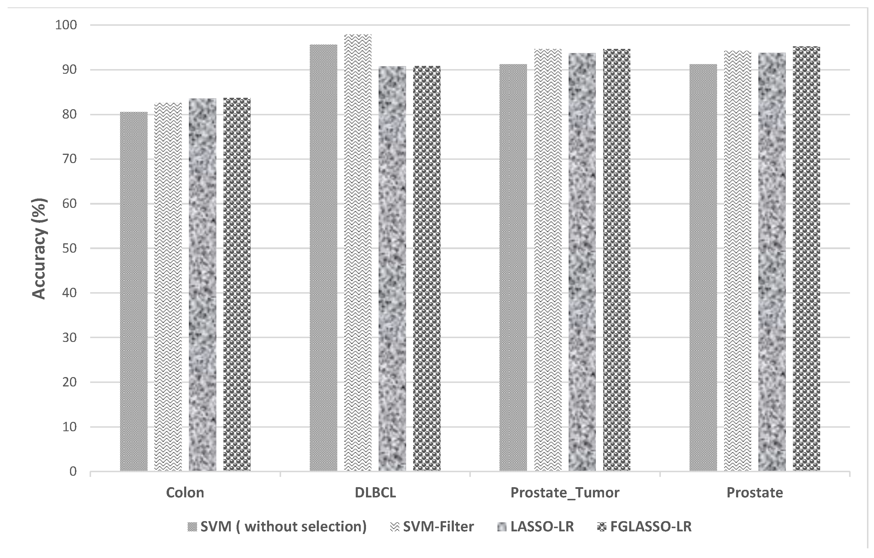
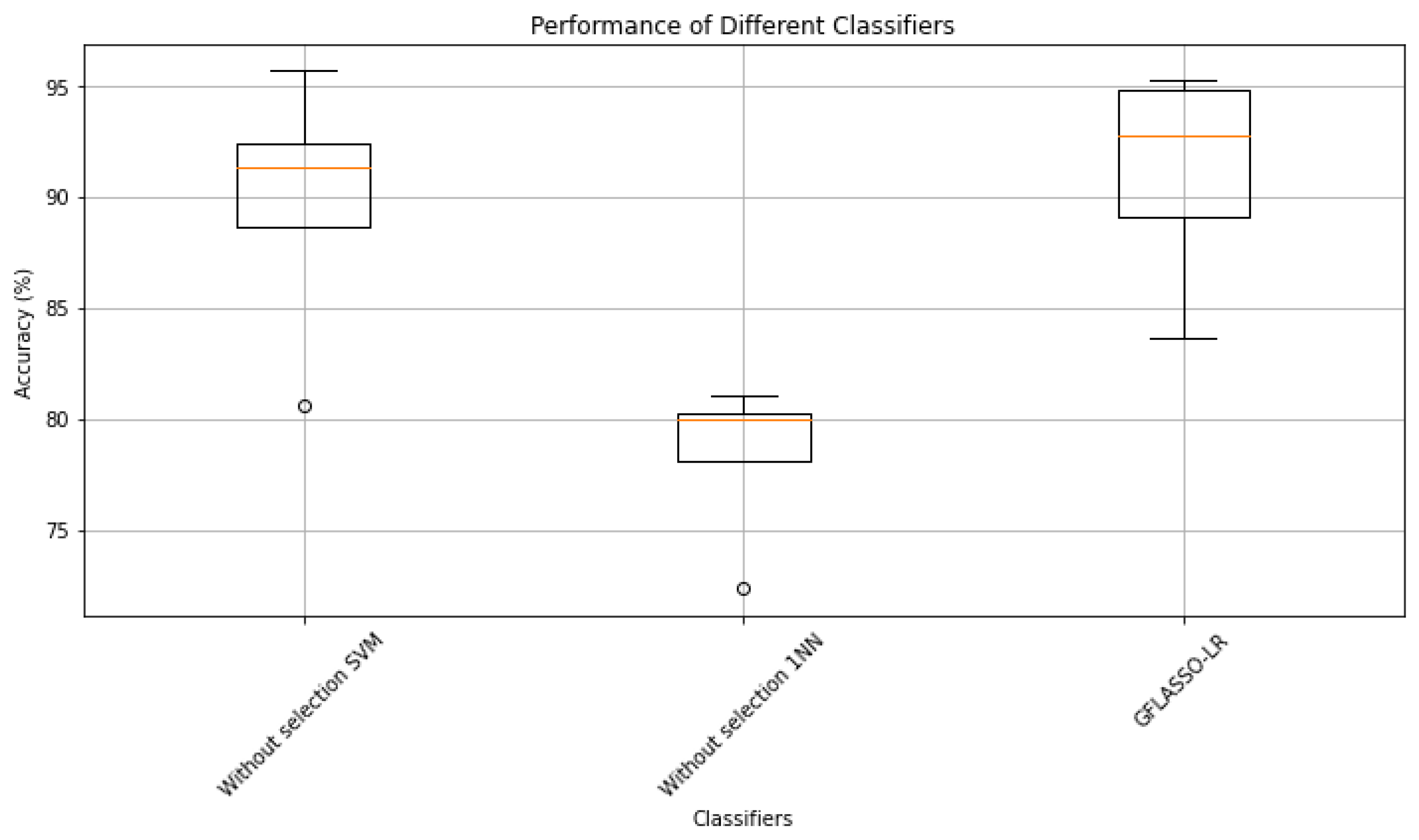
3.3. Results and Comparisons
- , which corresponds to a LASSO-LR type penalty.
- , which corresponds to a generalized Fused LASSO (GFLASSO-LR) type penalty.
Comparison with Other Approaches
3.4. Time and Memory Complexity
3.4.1. Pre-Processing Step (Selecting the Top 200 Highest-Ranked Genes)
- Time Complexity: Computing correlation coefficients for each gene across all samples and selecting the top 200 genes: (as provided in the information).
- Memory Complexity: Storing microarray data and correlation coefficients: .
3.4.2. Splitting-GFLASSO-LR Algorithm
- Time Complexity: for randomly splitting the dataset into training and test sets.
- Memory Complexity: for storing the training and test sets.
3.4.3. Building the Objective Function Based on the Training Data and the 200 Genes
3.4.4. Sub-Gradient Algorithm
- Constructing the graph and calculating weights: negligible compared to the overall complexity.
- Combining the subdifferentials: Once the subdifferentials of each component function are computed, they are combined according to the given expression. This involves a combination of nearly subdifferentials, resulting in a time complexity of .
- Iterating over the sub-gradient algorithm: iterations.
- Each iteration involves updating the coefficients using a sub-gradient: operations.
3.5. Discussion
4. Conclusions
Author Contributions
Funding
Data Availability Statement
Conflicts of Interest
References
- Li, M.; Ke, L.; Wang, L.; Deng, S.; Yu, X. A novel hybrid gene selection for tumor identification by combining multifilter integration and a recursive flower pollination search algorithm. Knowl.-Based Syst. 2023, 262, 110250. [Google Scholar] [CrossRef]
- Feng, S.; Jiang, X.; Huang, Z.; Li, F.; Wang, R.; Yuan, X.; Sun, Z.; Tan, H.; Zhong, L.; Li, S.; et al. DNA methylation remodeled amino acids biosynthesis regulates flower senescence in carnation (Dianthus caryophyllus). New Phytol. 2024, 241, 1605–1620. [Google Scholar] [CrossRef] [PubMed]
- Mehrabi, N.; Haeri Boroujeni, S.P.; Pashaei, E. An efficient high-dimensional gene selection approach based on the Binary Horse Herd Optimization Algorithm for biologicaldata classification. Iran J. Comput. Sci. 2024, 1–31. [Google Scholar] [CrossRef]
- Syu, G.D.; Dunn, J.; Zhu, H. Developments and applications of functional protein microarrays. Mol. Cell. Proteom. 2020, 19, 916–927. [Google Scholar] [CrossRef] [PubMed]
- Caraffi, S.G.; van der Laan, L.; Rooney, K.; Trajkova, S.; Zuntini, R.; Relator, R.; Haghshenas, S.; Levy, M.A.; Baldo, C.; Mandrile, G.; et al. Identification of the DNA methylation signature of Mowat-Wilson syndrome. Eur. J. Hum. Genet. 2024, 1–11. [Google Scholar] [CrossRef] [PubMed]
- Srivastava, S.; Jayaswal, N.; Kumar, S.; Sharma, P.K.; Behl, T.; Khalid, A.; Mohan, S.; Najmi, A.; Zoghebi, K.; Alhazmi, H.A. Unveiling the potential of proteomic and genetic signatures for precision therapeutics in lung cancer management. Cell. Signal. 2024, 113, 110932. [Google Scholar] [CrossRef]
- Ghavidel, A.; Pazos, P. Machine learning (ML) techniques to predict breast cancer in imbalanced datasets: A systematic review. J. Cancer Surviv. 2023, 1–25. [Google Scholar] [CrossRef]
- Bir-Jmel, A.; Douiri, S.M.; Elbernoussi, S. Gene selection via a new hybrid ant colony optimization algorithm for cancer classification in high-dimensional data. Comput. Math. Methods Med. 2019, 2019, 7828590. [Google Scholar] [CrossRef] [PubMed]
- Bir-Jmel, A.; Douiri, S.M.; Elbernoussi, S. Gene selection via BPSO and Backward generation for cancer classification. RAIRO-Oper. Res. 2019, 53, 269–288. [Google Scholar] [CrossRef]
- Sethi, B.K.; Singh, D.; Rout, S.K.; Panda, S.K. Long Short-Term Memory-Deep Belief Network based Gene Expression Data Analysis for Prostate Cancer Detection and Classification. IEEE Access 2023, 12, 1508–1524. [Google Scholar] [CrossRef]
- Maafiri, A.; Bir-Jmel, A.; Elharrouss, O.; Khelifi, F.; Chougdali, K. LWKPCA: A New Robust Method for Face Recognition Under Adverse Conditions. IEEE Access 2022, 10, 64819–64831. [Google Scholar] [CrossRef]
- Bir-Jmel, A.; Douiri, S.M.; Elbernoussi, S. Minimum redundancy maximum relevance and VNS based gene selection for cancer classification in high-dimensional data. Int. J. Comput. Sci. Eng. 2024, 27, 78–89. [Google Scholar]
- Maafiri, A.; Chougdali, K. Robust face recognition based on a new Kernel-PCA using RRQR factorization. Intell. Data Anal. 2021, 25, 1233–1245. [Google Scholar] [CrossRef]
- Amaldi, E.; Kann, V. On the approximability of minimizing nonzero variables or unsatisfied relations in linear systems. Theor. Comput. Sci. 1998, 209, 237–260. [Google Scholar] [CrossRef]
- Blum, A.L.; Rivest, R.L. Training a 3-node neural network is NP-complete. Neural Netw. 1992, 5, 117–127. [Google Scholar] [CrossRef]
- Yaqoob, A.; Verma, N.K.; Aziz, R.M. Optimizing gene selection and cancer classification with hybrid sine cosine and cuckoo search algorithm. J. Med. Syst. 2024, 48, 10. [Google Scholar] [CrossRef] [PubMed]
- Bechar, A.; Elmir, Y.; Medjoudj, R.; Himeur, Y.; Amira, A. Harnessing transformers: A leap forward in lung cancer image detection. In Proceedings of the 2023 6th International Conference on Signal Processing and Information Security (ICSPIS), Dubai, United Arab Emirates, 8–9 November 2023; pp. 218–223. [Google Scholar]
- Hamza, A.; Lekouaghet, B.; Himeur, Y. Hybrid whale-mud-ring optimization for precise color skin cancer image segmentation. In Proceedings of the 2023 6th International Conference on Signal Processing and Information Security (ICSPIS), Dubai, United Arab Emirates, 8–9 November 2023; pp. 87–92. [Google Scholar]
- Habchi, Y.; Himeur, Y.; Kheddar, H.; Boukabou, A.; Atalla, S.; Chouchane, A.; Ouamane, A.; Mansoor, W. Ai in thyroid cancer diagnosis: Techniques, trends, and future directions. Systems 2023, 11, 519. [Google Scholar] [CrossRef]
- Kohavi, R.; John, G.H. Wrappers for feature subset selection. Artif. Intell. 1997, 97, 273–324. [Google Scholar] [CrossRef]
- Gu, Q.; Li, Z.; Han, J. Generalized fisher score for feature selection. arXiv 2012, arXiv:1202.3725. [Google Scholar]
- Jafari, P.; Azuaje, F. An assessment of recently published gene expression data analyses: Reporting experimental design and statistical factors. BMC Med. Inform. Decis. Mak. 2006, 6, 27. [Google Scholar] [CrossRef]
- Mishra, D.; Sahu, B. Feature selection for cancer classification: A signal-to-noise ratio approach. Int. J. Sci. Eng. Res. 2011, 2, 1–7. [Google Scholar]
- Wang, Z. Neuro-Fuzzy Modeling for Microarray Cancer Gene Expression Data; First year transfer report; University of Oxford: Oxford, UK, 2005. [Google Scholar]
- Kononenko, I. Estimating attributes: Analysis and extensions of RELIEF. In European Conference on Machine Learning; Springer: Berlin/Heidelberg, Germany, 1994; pp. 171–182. [Google Scholar]
- Kishore, A.; Venkataramana, L.; Prasad, D.V.V.; Mohan, A.; Jha, B. Enhancing the prediction of IDC breast cancer staging from gene expression profiles using hybrid feature selection methods and deep learning architecture. Med. Biol. Eng. Comput. 2023, 61, 2895–2919. [Google Scholar] [CrossRef] [PubMed]
- Du, J.; Zhang, Z.; Sun, Z. Variable selection for partially linear varying coefficient quantile regression model. Int. J. Biomath. 2013, 6, 1350015. [Google Scholar] [CrossRef]
- Li, C.J.; Zhao, H.M.; Dong, X.G. Bayesian empirical likelihood and variable selection for censored linear model with applications to acute myelogenous leukemia data. Int. J. Biomath. 2019, 12, 1950050. [Google Scholar] [CrossRef]
- Li, L.; Liu, Z.P. Biomarker discovery from high-throughput data by connected network-constrained support vector machine. Expert Syst. Appl. 2023, 226, 120179. [Google Scholar] [CrossRef]
- Alharthi, A.M.; Lee, M.H.; Algamal, Z.Y. Gene selection and classification of microarray gene expression data based on a new adaptive L1-norm elastic net penalty. Inform. Med. Unlocked 2021, 24, 100622. [Google Scholar] [CrossRef]
- Alharthi, A.M.; Lee, M.H.; Algamal, Z.Y. Weighted L1-norm logistic regression for gene selection of microarray gene expression classification. Int. J. Adv. Sci. Eng. Inf. Technol. 2020, 4, 2088–5334. [Google Scholar] [CrossRef]
- Algamal, Z.Y.; Lee, M.H. Penalized logistic regression with the adaptive LASSO for gene selection in high-dimensional cancer classification. Expert Syst. Appl. 2015, 42, 9326–9332. [Google Scholar] [CrossRef]
- Algamal, Z.Y.; Lee, M.H. A two-stage sparse logistic regression for optimal gene selection in high-dimensional microarray data classification. Adv. Data Anal. Classif. 2019, 13, 753–771. [Google Scholar] [CrossRef]
- Li, L.; Liu, Z.P. A connected network-regularized logistic regression model for feature selection. Appl. Intell. 2022, 52, 11672–11702. [Google Scholar] [CrossRef]
- Yang, Z.Y.; Liang, Y.; Zhang, H.; Chai, H.; Zhang, B.; Peng, C. Robust Sparse Logistic Regression with the Lq(0 < q < 1) Regularization for Feature Selection Using Gene Expression Data. IEEE Access 2018, 6, 68586–68595. [Google Scholar]
- Ijaz, M.; Asghar, Z.; Gul, A. Ensemble of penalized logistic models for classification of high-dimensional data. Commun.-Stat.-Simul. Comput. 2019, 50, 2072–2088. [Google Scholar] [CrossRef]
- Kastrin, A.; Peterlin, B. Rasch-based high-dimensionality data reduction and class prediction with applications to microarray gene expression data. Expert Syst. Appl. 2010, 37, 5178–5185. [Google Scholar] [CrossRef]
- Wang, Y.; Zhang, W.; Fan, M.; Ge, Q.; Qiao, B.; Zuo, X.; Jiang, B. Regression with Adaptive Lasso and Correlation based Penalty. Appl. Math. Model. 2021, 105, 179–196. [Google Scholar] [CrossRef]
- Zou, H.; Hastie, T. Regularization and variable selection via the elastic net. J. R. Stat. Soc. Ser. B Stat. Methodol. 2005, 67, 301–320. [Google Scholar] [CrossRef]
- Zou, H. The adaptive lasso and its oracle properties. J. Am. Stat. Assoc. 2006, 101, 1418–1429. [Google Scholar] [CrossRef]
- Bach, F.; Jenatton, R.; Mairal, J.; Obozinski, G. Structured sparsity through convex optimization. Stat. Sci. 2012, 27, 450–468. [Google Scholar] [CrossRef]
- Tibshirani, R.; Saunders, M.; Rosset, S.; Zhu, J.; Knight, K. Sparsity and smoothness via the fused lasso. J. R. Stat. Soc. Ser. B Stat. Methodol. 2005, 67, 91–108. [Google Scholar] [CrossRef]
- Jang, W.; Lim, J.; Lazar, N.A.; Loh, J.M.; Yu, D. Some properties of generalized fused lasso and its applications to high dimensional data. J. Korean Stat. Soc. 2015, 44, 352–365. [Google Scholar] [CrossRef]
- Rinaldo, A. Properties and refinements of the fused lasso. Ann. Stat. 2009, 37, 2922–2952. [Google Scholar] [CrossRef]
- Qian, J.; Jia, J. On stepwise pattern recovery of the fused lasso. Comput. Stat. Data Anal. 2016, 94, 221–237. [Google Scholar] [CrossRef]
- Höfling, H.; Binder, H.; Schumacher, M. A coordinate-wise optimization algorithm for the Fused Lasso. arXiv 2010, arXiv:1011.6409. [Google Scholar]
- Viallon, V.; Lambert-Lacroix, S.; Hoefling, H.; Picard, F. On the robustness of the generalized fused lasso to prior specifications. Stat. Comput. 2016, 26, 285–301. [Google Scholar] [CrossRef]
- Hoefling, H. A path algorithm for the fused lasso signal approximator. J. Comput. Graph. Stat. 2010, 19, 984–1006. [Google Scholar] [CrossRef]
- Liu, J.; Yuan, L.; Ye, J. An efficient algorithm for a class of fused lasso problems. In Proceedings of the 16th ACM SIGKDD International Conference on Knowledge Discovery and Data Mining, Washington, DC, USA, 25–28 July 2010; pp. 323–332. [Google Scholar]
- Tibshirani, R.J.; Taylor, J. The solution path of the generalized lasso. Ann. Stat. 2011, 39, 1335–1371. [Google Scholar] [CrossRef]
- Johnson, N.A. A dynamic programming algorithm for the fused lasso and l 0-segmentation. J. Comput. Graph. Stat. 2013, 22, 246–260. [Google Scholar] [CrossRef]
- Fisher, R.A.; Yates, F. Statistical Tables for Biological, Agricultural and Medical Research; Oliver and Boyd: Edinburgh, UK, 1938. [Google Scholar]
- Albert, A.; Anderson, J.A. On the existence of maximum likelihood estimates in logistic regression models. Biometrika 1984, 71, 1–10. [Google Scholar] [CrossRef]
- Liang, Y.; Liu, C.; Luan, X.Z.; Leung, K.S.; Chan, T.M.; Xu, Z.B.; Zhang, H. Sparse logistic regression with a L1/2 penalty for gene selection in cancer classification. BMC Bioinform. 2013, 14, 198. [Google Scholar] [CrossRef] [PubMed]
- Hoerl, A.E.; Kennard, R.W. Ridge regression: Biased estimation for nonorthogonal problems. Technometrics 1970, 12, 55–67. [Google Scholar] [CrossRef]
- Tibshirani, R. Regression shrinkage and selection via the lasso. J. R. Stat. Soc. Ser. B Methodol. 1996, 58, 267–288. [Google Scholar] [CrossRef]
- Meinshausen, N. Relaxed lasso. Comput. Stat. Data Anal. 2007, 52, 374–393. [Google Scholar] [CrossRef]
- Meier, L.; Van De Geer, S.; Bühlmann, P. The group lasso for logistic regression. J. R. Stat. Soc. Ser. B Stat. Methodol. 2008, 70, 53–71. [Google Scholar] [CrossRef]
- Wang, S.; Nan, B.; Rosset, S.; Zhu, J. Random lasso. Ann. Appl. Stat. 2011, 5, 468. [Google Scholar] [CrossRef]
- Shor, N.Z. Application of the gradient-descent method to solution of the network transport problem. Cybern. Syst. Anal. 1967, 3, 43–45. [Google Scholar] [CrossRef]
- Polyak, B.T. Minimization of unsmooth functionals. USSR Comput. Math. Math. Phys. 1969, 9, 14–29. [Google Scholar] [CrossRef]
- Nemirovski, A.S.; Yudin, D.B. Cesari convergence of the gradient method of approximating saddle points of convex-concave functions. Dokl. Akad. Nauk. SSSR 1978, 239, 1056–1059. [Google Scholar]
- Rockafellar, R.T. Convex Analysis; Princeton University Press: Princeton, NJ, USA, 1970. [Google Scholar]
- Anstreicher, K.M.; Wolsey, L.A. Two “well-known” properties of subgradient optimization. Math. Program. 2009, 120, 213–220. [Google Scholar] [CrossRef]
- Polyak, B.T. A general method for solving extremal problems. Dokl. Akad. Nauk. SSSR 1967, . 174, 33–36. [Google Scholar]
- Shor, N.Z. Minimization Methods for Non-Differentiable Functions; Springer Science & Business Media: Berlin, Germany, 2012; Volume 3. [Google Scholar]
- Mordukhovich, B.S.; Nam, N.M. An Easy Path to Convex Analysis and Applications; Synthesis Lectures on Mathematics and Statistics; Springer: Cham, Switzerland, 2013; Volume 6. [Google Scholar]
- Huang, J.; Ma, S.; Zhang, C.H. The Iterated Lasso for High-Dimensional Logistic Regression; Technical report; The University of Iowa, Department of Statistics and Actuarial Sciences: Iowa City, IA, USA, 2008. [Google Scholar]
- Cui, L.; Bai, L.; Wang, Y.; Philip, S.Y.; Hancock, E.R. Fused lasso for feature selection using structural information. Pattern Recognit. 2021, 119, 108058. [Google Scholar] [CrossRef]
- Bertsekas, D.P. Nonlinear programming. J. Oper. Res. Soc. 1997, 48, 334. [Google Scholar] [CrossRef]
- Alon, U.; Barkai, N.; Notterman, D.A.; Gish, K.; Ybarra, S.; Mack, D.; Levine, A.J. Broad patterns of gene expression revealed by clustering analysis of tumor and normal colon tissues probed by oligonucleotide arrays. Proc. Natl. Acad. Sci. USA 1999, 96, 6745–6750. [Google Scholar] [CrossRef] [PubMed]
- Statnikov, A.; Aliferis, C.F.; Tsamardinos, I.; Hardin, D.; Levy, S. A comprehensive evaluation of multicategory classification methods for microarray gene expression cancer diagnosis. Bioinformatics 2005, 21, 631–643. [Google Scholar] [CrossRef] [PubMed]
- Singh, D.; Febbo, P.G.; Ross, K.; Jackson, D.G.; Manola, J.; Ladd, C.; Tamayo, P.; Renshaw, A.A.; D’Amico, A.V.; Richie, J.P.; et al. Gene expression correlates of clinical prostate cancer behavior. Cancer Cell 2002, 1, 203–209. [Google Scholar] [CrossRef] [PubMed]
- Alber, Y.I.; Iusem, A.N.; Solodov, M.V. On the projected subgradient method for nonsmooth convex optimization in a Hilbert space. Math. Program. 1998, 81, 23–35. [Google Scholar] [CrossRef]
- Algamal, Z.Y.; Alhamzawi, R.; Ali, H.T.M. Gene selection for microarray gene expression classification using Bayesian Lasso quantile regression. Comput. Biol. Med. 2018, 97, 145–152. [Google Scholar] [CrossRef]
- Fan, J.; Li, R. Variable selection via nonconcave penalized likelihood and its oracle properties. J. Am. Stat. Assoc. 2001, 96, 1348–1360. [Google Scholar] [CrossRef]


| Reference | Methodological Approach | Application Area | Challenges Addressed | Notable Contributions |
|---|---|---|---|---|
| Li et al. [1] | High-dimensional data analysis | DNA microarray data | Statistical analysis difficulty in classification tasks | Developed approaches for gene subset identification |
| Feng et al. [2] | High-dimensional data analysis | DNA microarray data | High-dimensional data challenges in gene selection | Improved understanding of gene–disease relationships |
| Mehrabi et al. [3] | Efficient gene selection methods | DNA microarray data | Curse of dimensionality in microarray data analysis | Enhanced classification accuracy for diseases like cancer |
| Syu et al. [4] | Microarray technology analysis | Medicine and Biology | Clinical diagnosis and gene co-regulation | Identified critical genes for tumor growth and diagnostic systems development |
| Caraffi et al. [5] | Microarray data analysis | Cancer research | Computational and biological challenges | Developed diagnostic systems to aid in cancer treatment |
| Ghavidel et al. [7] | Machine learning approaches | Microarray data analysis | Computational instability and sample size limitation | Addressed the curse of dimensionality with computational methods |
| Birjmel et al. [12] | Optimization methods for gene selection | DNA microarray data | Gene-sample number disparity | Advanced optimization methods to improve classifier quality |
| Yaqoob et al. [16] | Gene selection for personalized medicine | Cancer research | Need for high classification accuracy | Optimized gene selection methods for better physician decision-making |
| Alharthi et al. [30] | Regularized methods, PLR with LASSO | Cancer classification | Limitations of LASSO | Introduced Elastic-Net (EN) and adaptive LASSO (ALASSO) for cancer classification |
| Zou et al. [40] | Adaptive LASSO | Statistical analysis | Oracle property deficiencies in LASSO | Introduced weights for penalization within the norm |
| Hofling et al. [46] | Generalized Fused LASSO (GFLASSO) | Linear regression | Challenges in norm penalties minimization | Penalized coefficient differences based on a gene graph for sparse solutions |
| Dataset | # Genes | # Samples | # Classes | Source |
|---|---|---|---|---|
| Colon | 2000 | 62 | 2 | [71] |
| DLBCL | 5469 | 77 | 2 | [72] |
| Prostate_Tumor | 10,509 | 102 | 2 | [72] |
| Prostate | 12,600 | 102 | 2 | [73] |
| 0.05 | 0.15 | 0.25 | 0.35 | 0.45 | 0.55 | 0.65 | 0.75 | 0.85 | 0.95 | 1 | |
| The optimal value | 12.49 | 8.61 | 7.38 | 7.13 | 7.04 | 7.01 | 7.01 | 7.15 | 8.02 | 15.42 | 19.72 |
| Accuracy (Test) | Number of Genes | |
|---|---|---|
| 0.2 | 96.14 | 55.6 |
| 0.4 | 96.1 | 36.8 |
| 0.6 | 96.14 | 32.6 |
| 0.8 | 96.14 | 29 |
| 1 | 96.14 | 24 |
| 1.2 | 97.1 | 28 |
| 1.4 | 96.14 | 26.2 |
| 1.6 | 97.1 | 25.4 |
| 1.8 | 96.14 | 25.6 |
| 2 | 96.14 | 22.6 |
| 2.2 | 96.14 | 24.6 |
| 2.4 | 96.14 | 23.8 |
| 2.6 | 95.14 | 22.2 |
| 2.8 | 96.14 | 20.4 |
| 3 | 95.14 | 20.8 |
| 3.2 | 94.19 | 20.4 |
| 3.4 | 94.19 | 20.4 |
| 3.6 | 94.19 | 20.4 |
| 3.8 | 95.14 | 19.6 |
| 4 | 94.19 | 19.2 |
| Accuracy (Test) | Number of Genes | |
|---|---|---|
| 0 | 94.19 | 21.6 |
| 0.025 | 96.14 | 20 |
| 0.05 | 96.14 | 21.2 |
| 0.075 | 96.14 | 22.4 |
| 0.1 | 97.1 | 22 |
| 0.125 | 97.1 | 23.8 |
| 0.15 | 97.1 | 24 |
| 0.175 | 96.14 | 25 |
| 0.2 | 97.1 | 25.4 |
| 0.225 | 95.14 | 25.6 |
| 0.25 | 97.1 | 26.6 |
| 0.275 | 95.14 | 28.2 |
| 0.3 | 95.19 | 27.4 |
| 0.325 | 95.14 | 28.4 |
| 0.35 | 95.14 | 28.6 |
| 0.375 | 95.19 | 27.2 |
| 0.4 | 96.14 | 27.2 |
| 0.425 | 96.14 | 28.4 |
| 0.45 | 96.14 | 25.8 |
| 0.475 | 96.14 | 28.6 |
| 0.5 | 95.19 | 28.2 |
| 0.525 | 95.1 | 29.6 |
| 0.55 | 97.1 | 27 |
| 0.575 | 95.14 | 30.8 |
| 0.6 | 96.19 | 29.6 |
| 0.625 | 95.19 | 28.2 |
| 0.65 | 95.19 | 32.2 |
| 0.675 | 96.1 | 31.2 |
| 0.7 | 94.14 | 26.8 |
| 0.725 | 96.14 | 29.8 |
| 0.75 | 95.19 | 29.2 |
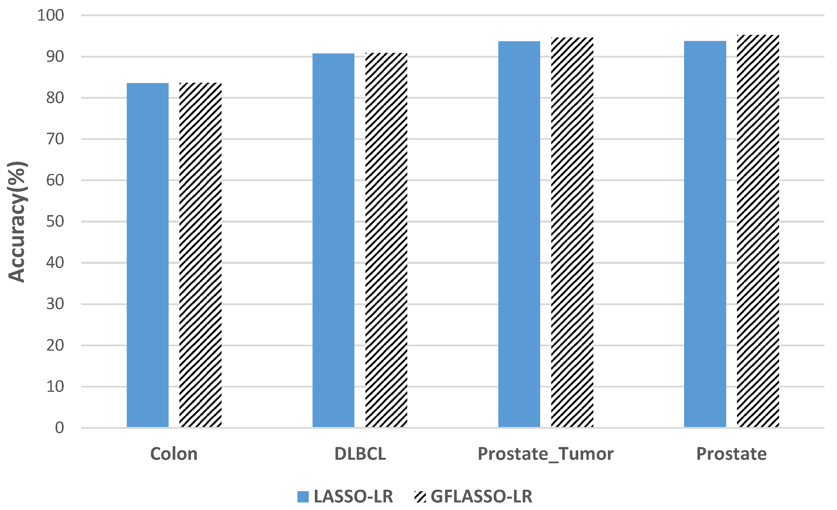
| Dataset | Performance | Without Selection | Pearson Filter | LASSO-LR | GFLASSO-LR | ||
|---|---|---|---|---|---|---|---|
| 1NN | SVM | 1NN | SVM | ||||
| Colon | Accuracy (%) | 72.33 | 80.56 | 80.66 | 82.55 | 83.56 | 83.67 |
| Number of genes | 2000 | 200 | 15.4 | 19.9 | |||
| DLBCL | Accuracy (%) | 81.04 | 95.65 | 95.47 | 97.91 | 90.78 | 90.87 |
| Number of genes | 5469 | 200 | 21.24 | 20.4 | |||
| Prostate_Tumor | Accuracy (%) | 80 | 91.27 | 90.86 | 94.6 | 93.73 | 94.6 |
| Number of genes | 10,509 | 200 | 20.66 | 21.34 | |||
| Prostate | Accuracy (%) | 80 | 91.27 | 91.73 | 94.26 | 93.8 | 95.27 |
| Number of genes | 12,600 | 200 | 20.64 | 20.94 | |||
| Dataset | Performences | GFLASSO-LR (Our Method) | BLASSO [75] | LASSO [56] | SCAD [76] | ALASSO [40] | Nouvel ALASSO [31] |
CBPLR [32] |
|---|---|---|---|---|---|---|---|---|
| Colon | Acccuracy (%) | 83.67 < 2 > | 93 | 79.53 | 79.51 | 78.4 | 82.91 | 89.5 |
| Number of genes | 19.9 | 11 | 14 | 14 | 14 | 12 | 10 | |
| DLBCL | Acccuracy (%) | 90.87 < 3 > | 84 | 88.33 | 74.02 | 84.41 | 91.32 | 91.7 |
| Number of genes | 20.4 | 17 | 24 | 24 | 24 | 22 | 17 | |
| Prostate | Acccuracy (%) | 95.27 < 1 > | - | 91.14 | 60.13 | 82.11 | 93.53 | 93.6 |
| Number of genes | 20.94 | - | 29 | 28 | 28 | 24 | 16 |
Disclaimer/Publisher’s Note: The statements, opinions and data contained in all publications are solely those of the individual author(s) and contributor(s) and not of MDPI and/or the editor(s). MDPI and/or the editor(s) disclaim responsibility for any injury to people or property resulting from any ideas, methods, instructions or products referred to in the content. |
© 2024 by the authors. Licensee MDPI, Basel, Switzerland. This article is an open access article distributed under the terms and conditions of the Creative Commons Attribution (CC BY) license (https://creativecommons.org/licenses/by/4.0/).
Share and Cite
Bir-Jmel, A.; Douiri, S.M.; Bernoussi, S.E.; Maafiri, A.; Himeur, Y.; Atalla, S.; Mansoor, W.; Al-Ahmad, H. GFLASSO-LR: Logistic Regression with Generalized Fused LASSO for Gene Selection in High-Dimensional Cancer Classification. Computers 2024, 13, 93. https://doi.org/10.3390/computers13040093
Bir-Jmel A, Douiri SM, Bernoussi SE, Maafiri A, Himeur Y, Atalla S, Mansoor W, Al-Ahmad H. GFLASSO-LR: Logistic Regression with Generalized Fused LASSO for Gene Selection in High-Dimensional Cancer Classification. Computers. 2024; 13(4):93. https://doi.org/10.3390/computers13040093
Chicago/Turabian StyleBir-Jmel, Ahmed, Sidi Mohamed Douiri, Souad El Bernoussi, Ayyad Maafiri, Yassine Himeur, Shadi Atalla, Wathiq Mansoor, and Hussain Al-Ahmad. 2024. "GFLASSO-LR: Logistic Regression with Generalized Fused LASSO for Gene Selection in High-Dimensional Cancer Classification" Computers 13, no. 4: 93. https://doi.org/10.3390/computers13040093
APA StyleBir-Jmel, A., Douiri, S. M., Bernoussi, S. E., Maafiri, A., Himeur, Y., Atalla, S., Mansoor, W., & Al-Ahmad, H. (2024). GFLASSO-LR: Logistic Regression with Generalized Fused LASSO for Gene Selection in High-Dimensional Cancer Classification. Computers, 13(4), 93. https://doi.org/10.3390/computers13040093