Abstract
Crabs and lobsters are valuable crustaceans that contribute enormously to the seafood needs of the growing human population. This paper presents a comprehensive analysis of single- and multi-stage object detectors for the detection of crabs and lobsters using images captured onboard fishing boats. We investigate the speed and accuracy of multiple object detection techniques using a novel dataset, multiple backbone networks, various input sizes, and fine-tuned parameters. We extend our work to train lightweight models to accommodate the fishing boats equipped with low-power hardware systems. Firstly, we train Faster R-CNN, SSD, and YOLO with different backbones and tuning parameters. The models trained with higher input sizes resulted in lower frames per second (FPS) and vice versa. The base models were highly accurate but were compromised in computational and run-time costs. The lightweight models were adaptable to low-power hardware compared to the base models. Secondly, we improved the performance of YOLO (v3, v4, and tiny versions) using custom anchors generated by the k-means clustering approach using our novel dataset. The YOLO (v4 and it’s tiny version) achieved mean average precision (mAP) of 99.2% and 95.2%, respectively. The YOLOv4-tiny trained on the custom anchor-based dataset is capable of precisely detecting crabs and lobsters onboard fishing boats at 64 frames per second (FPS) on an NVidia GeForce RTX 3070 GPU. The Results obtained identified the strengths and weaknesses of each method towards a trade-off between speed and accuracy for detecting objects in input images.
1. Introduction
1.1. Background and Motivation
Fisheries-related data are of great importance to fishery organisations worldwide. The consequences of data not being captured and stored appropriately result in incorrect stock reporting that leads to overfishing, which is contrary to the ecological integrity of the ocean. One of the initial steps in this procedure is data collection and analysis, which is crucial for making well-informed decisions [1]. A lack of accurate data causes uncertainties, and improving data quality is beneficial for marine scientists and for fish stock management. Technologies and modern scientific procedures have already improved the level of data collection for most fisheries. We investigate deep learning methods for collecting data on crabs and lobsters onboard fishing boats. These two valuable crustaceans have gained less attention from computer scientists in the past.
The purpose of collecting fisheries data is to monitor commercial fishing, and in this work, we focus on smaller independent fishers, which are more difficult to monitor and require that any automated solution be low-cost and unobtrusive on smaller fishing vessels. The data can include information on catch, bycatch, landings, discard, location, and the biological or demographic composition of a catch, like sexing and DNA sampling, fishing efforts, fishing gears, protected species interactions, coverage, counting, size estimation, weight, date, time, etc.
One of the conventional methods for collecting fisheries data involves onboard observers, who are placed onboard for monitoring, compliance, and scientific assessments of fish stocks [2]. Each country has its own fisheries observer programme, and hence the roles of observers vary worldwide. They can play the dual roles of collecting data and reporting on compliance under the fisheries regulations in the country. Other methods include vessel monitoring systems, electronic monitoring (EM), electronic reporting, logbooks, mobile computing, fishing surveys, questionnaires, etc. Each method has its strengths and limitations that impact the quality of data obtained. Combining tools for building integrated systems can optimise the accuracy of the fisheries estimates in a real-time manner [3].
Artificial intelligence (AI) has demonstrated remarkable results in solving complex computational problems with computer-based learning approaches such as machine learning (ML) algorithms, in particular deep neural networks. These networks are trained using given datasets and, once trained, can efficiently produce outputs for unseen data and events. Some countries, including the UK, are collecting on-site visual data of catch events through EM and mobile computing [4,5]. These data can be used to train networks to automate the catch recognition and measurement of species. Automated image analysis techniques can address these problems and find appropriate solutions through easier access to data and monitoring of the catch events onboard vessels. Unlike other fields, AI is not yet extensively integrated into fisheries applications [6]. However, marine biologists and management recommend that new automated real-time data collection programmes will help improve the current standards of data collection practices [4].
The ease of access to computer resources, cost reduction, availability of datasets, and improved algorithms have increased the use of computer-based solutions in the recent decade. This is a motivation for computer science researchers to develop computer vision systems for the fishing sector around the globe. Developed countries are incorporating modern machine learning and computer vision-based applications into their fisheries setups, while others rely on alternate options to improve the current standards of fishing data. The ultimate goal is to respond to the seafood needs of the people and to maintain the integrity of aquatic life.
Collaboration between fishers, marine scientists, and computer scientists is required to make effective use of the new technological opportunities. Integration of AI, data science, and information technology will support building state-of-the-art applications for both aquaculture and capture fisheries [7]. The United Nation’s “Decade of the Ocean” theme [8] aims to achieve a healthy, safe, and resilient ocean by 2030, where AI can play a pivotal role in making this theme practical. This will initiate new opportunities for interdisciplinary collaborations to promote AI-based marine research and development.
Hold et al. [4] evaluated the use of onboard camera systems for collecting crab and lobster data. GoPro cameras mounted on fishing boats recorded images of crabs and lobsters. Multiple fishers and onboard observers passed the animals on the designated area for comparison between the in situ and predicted values of the measurements of the animals. This was a step towards finding the size and sex of crabs and lobsters through analysis of the recordings of onboard camera systems. Collecting data without onboard observers reduces the cost, and computer automation of image extraction and measurements will further enhance the utility of video systems for data collection. This motivated us to proceed with our research on computer vision-based automated detection and measurement of crabs and lobsters onboard fishing boats. We worked in collaboration with marine scientists and fishermen from Bangor University, UK. They provided us with onboard fishing videos, which our research utilises for the training and testing of networks [9,10]. We created a large dataset of 15,100 images of crabs and lobsters, which was used to train and test our models for detection of crabs and lobsters on fishing boats. The dataset is unique and contains both the animals in equal proportions of 50% each. Detail about the dataset creation is given in Section 3.
The selected two crustaceans have received less attention in scientific research; thus, this paper contributes towards filling this gap and promoting computer vision-based solutions for investigating different aspects of fisheries data. Our contributions in this paper include the following: (1) the detailed evaluation of one- and two-stage object detectors; (2) the creation of large datasets used for the application of crab and lobster detection onboard fishing boats; (3) the presentation of both low-power and high-power hardware solutions for the detection problem; and (4) improvements in the results of the YOLOv4 base and tiny models using custom anchors and a novel dataset.
1.2. Related Work
1.2.1. Object Detection
This paper focuses on the detection of crabs and lobsters using images captured onboard fishing boats. The lack of published research on collecting data on crabs and lobsters prompted us to investigate deep learning as a potential solution. Biologists, marine scientists, and fishery organisations advise computer automation of data gathering and monitoring to enhance the effectiveness of current systems deployed on fishing boats. The video recordings of the fishing activities provided by our collaborators are used to create datasets for training and testing neural networks. We evaluated the performance of single- and multistage object detectors for identifying crabs and lobsters.
Object detection is an essential and challenging task of computer vision, with widespread applications in many disciplines. It is primarily a supervised learning problem that aims to localise all the instances of the pre-defined classes of the objects and display their outcome by drawing bounding boxes around the detections. Object detection serves other computer vision tasks like instance segmentation, image tracking, captioning, etc. The advent of sophisticated deep learning networks has improved the performance of object detectors for locating object classes in images and real-time videos [11]. Research to improve object detection tasks is growing in academia and industrial applications due to the development of Convolutional Neural Networks (CNNs), access to datasets, and the availability of faster GPUs (Graphics Processing Units). The fields of multi-class detection, edge detection, pose detection, face detection, crowd estimation, etc., are receiving more attention from researchers. Domain-specific object detectors are classified as one-stage, two-stage, few-shot, and transformer-based detectors. Most two-stage detectors achieve high localisation and object recognition accuracy, whereas one-stage detectors are highly responsive to real-time actions with increased inference speed. YOLO [12,13,14,15] and Faster R-CNN [16] are examples of one- and two-stage detectors, respectively. The transformers [17,18,19,20] were initially introduced for Natural Language Processing and have performed well in many vision tasks of classification and object detection, with the need for more training data. Few-Shot Object Detectors divide objects into base classes with too many training examples and novel classes with few examples, which suits the problem of having less training data.
1.2.2. Fish Detection
Electronic monitoring is widely used to monitor fisheries involving human analysts, with added cost and expense. Biologists are keen to implement ML systems as an alternative step towards automation and improvement. The first step in an automated pipeline of data capture is the detection of the catch, which executes the steps of classifying and localising the objects simultaneously.
Allken et al. [21] presented an image-based detection of pelagic (open sea) and mesopelagic (living at depths of 200–1000 m) fish types. The dataset images were captured with the DeepVision trawl camera system between 2017 and 2018 in the Norwegian Sea [22]. They used RetinaNet for the detection of the specified fish types. Using synthetic images to train the models achieved mAP of 84.5%. The RetinaNet-based object detector successfully automates locating and classifying fish species. This application contributed to collecting data on trawl fishing to quantify fish. Unlike tracking, the researchers used Deep Vision and a simple linear regression model to estimate fish counting of different classes. This strategy involves using the individual image frames classified by RetinaNet in the earlier step.
One-stage detectors are ideal for detecting objects in real-time applications. For example, Cai et al. [23] combined YOLOv3 and MobileNetV1 aiming to construct a detector with a lighter backbone for fish detection. The imageNet-based dataset was used with 16 different classes of fish species to pre-train the network. A dataset of 2000 images was split into 1700 and 300 images for training and testing, respectively. Their method achieved an AP (average precision) of 78.67%, which was better than that of the YOLOv3 base model for this specific problem of fish detection. Figure 1b shows detection images from [23].

Figure 1.
(a) automated catch event detection for longline fishing [24]; (b) fish detection results for YOLOv3 and MobileNetv1 [23].
An automatic fish detection system was proposed by Salman et al. [25] to detect moving fish objects in an unconstrained underwater environment using R-CNN. Their approach utilises fish motions in videos through background subtraction and optical flow. The outcomes combine with a raw image to obtain fish-dependent candidate regions. The experiments used FCS (Fish4Knowledge with Complex Scenes) and LCF-15 (LifeCLEF 2015) datasets with several underwater videos of different fish species. The base R-CNN produced an accuracy of 64.99% and 77.30% for the FCS and LCF-15 datasets, respectively. The proposed system attained a detection accuracy of 87.44% and 80.02% for the FCS and LCF-15 datasets, respectively, which were higher by 22.45% and 6.72%, respectively, than that for the base R-CNN.
EM involves recording catch events subsequently reviewed by analysts. The process consumes high storage space for recording and additional expense for the analysts. Qiao et al. [24] proposed an automated DL-based detector that allows recording catch events to overcome the limitations of EM. The authors examined multiple CNNs to extract features such as ResNet, DenseNet, and GoogLeNet. The fish and fisher detector adopted two frameworks of TensorBox progressive for human detection and YOLO for real-time processing. The datasets included 140 video recordings of pixels and a speed of 10 FPS. The proposed approach is completed in two steps. The first step detects fish and fishers in a frame-by-frame manner. The second step smooths occasional false and missing detections, identifying catch events and filtering unwanted or “empty” video frames. The trained system produced almost 100% accurate results when tested on footage from three longline fishing trips. The research aims to facilitate EM analysts in producing catch reports that are fast and accurate. Figure 1a shows detection images from [24].
Tseng and Kuo [26] presented a DL-based system for counting, measuring, and identifying fish types. The system detects harvested fish in EM video frames and segments them from the background using mask R-CNN. The counting involved time and distance threshold methods. The next step determines the fish measurement and classification using the masks predicted by mask R-CNN and confidence scores, respectively. The trained model achieved mAP of 93.51% and 77.31% for fish detection and counting, respectively. The accuracy of fish classification was above 98%. The proposed approach can automate pre-screening of EM videos to facilitate the process of video analysis by the analysts.
Acoustic signalling (a technique of sending and receiving messages for underwater communication) allows fisheries stock management and monitoring of marine life. It is a challenging task to assign it to the species. Trawl camera systems can implement the interpretation of acoustics data. The underwater images can help identify the presence of species at specific locations. Allken et al. proposed a DL neural network aiming to automate the classification of fish in images captured by the Deep Vision trawl camera system [22]. The dataset included images of multiple surveys conducted at 20 trawl stations using the Deep Vision system. Also, the authors developed a method for creating synthetic datasets. The proposed classifier used Tensorflow and Keras libraries and a fully convolutional Inception 3 network. The CNN-based system achieved 94% accuracy for identifying fish species of different types.
1.2.3. Crab and Lobster Detection
We include computer vision and image processing techniques for crab and lobster detection. The literature shows that these two crustaceans received less attention from scientists than fish and other species. Enough scope of research can explore new systems for automated data collection and monitoring of the two valuable species.
Crab aquaculture still relies on traditional methods to collect species data. Cao et al. [27] proposed a real-time robust underwater crab detector named Faster MSSDLite. The experiments involved 5125 images for training and testing the MSSDLite model. A combined lightweight SSD object detector and MobileNetV2 backbone were selected. A Feature Pyramid Network (FPN) was adopted to the SSD to boost the process of detection. The unified Quantized-CNN framework helped quantify the error and accelerate the speed. The proposed approach reported an AP of 98.94% and a detection speed of 74 FPS, 8× faster than SSD.
Accurate detection of crabs can promote the growth of the aquaculture industry at a rapid speed. Chin et al. [28] proposed a lightweight crab detection and sex classification method based on YOLOv4 named GMNet-YOLOv4. GhostNet was selected as a backbone to extract features from the crab images. The standard convolutions of the neck and head were replaced by depth-wise separable convolutions, reducing the network parameters. The modified trained model achieved mAP of 97.23%, which was 2.82% higher than the base model with lower memory consumption and reduced parameters.
Recently, Ji et al. [29] proposed a method to detect underwater river crabs. It was based on multi-scale pyramid fusion image enhancement using MobileCenterNet. The role of multi-scale pyramid fusion based on CLAHE (Contrast Limited Adaptive Histogram Equalization) and UDCP (Underwater Dark Channel Prior) is to enhance the image quality affected by poor light and low contrast in underwater setups. MobileNetV2 with added modules was applied to create feature maps. The MobileCenterNet achieved an AP of 97.86% and frame rate of 48 per second. The storage memory required for training the model was reduced by 81%, and the AP was increased by 3.2% compared to the baseline model ResNet18-CenterNet for a crab dataset of 3732 images.
Instead of considering the whole body of the crab, Wu et al. [30] proposed a DL approach based on abdomen parts for identification of swimming and mud crabs using two different datasets (Crab-201 and Crab-146). The proposed network, named PDN (Part-based Deep Learning Network) included three overlapping and non-overlapping partition strategies. Also, the edge texture of the abdomen is richer in features than the sulciform texture in the lower part of the abdomen. The technique of overlapping partitions and edge textures resulted in an improved mAP of 94.5% than the counterpart detectors for detecting specified crab species.
The detection of crabs in images has multiple applications in wider domains. Wang et al. [31] built an application to automate the meat picking process using CNN. The crab knuckle is a featured body part that addresses the size and position of the meat compartments of the crab, and it is important to have precise detection of the knuckle. The proposed work approaches the exact position of the knuckle in images. Initially, the background was removed from the images using the Otsu algorithm [32]. A CNN-based binary classification achieved an accuracy of 98.7% for the validation set. Other modifications for k-means clustering improved the ability to identify the exact knuckle position based on colour features of the back-fin area, and the use of template matching generated the cutline in the XY plane. The authors updated their work in a report published later [33]. They integrated the model into the crab processing machine. It detects crab legs, crab cores, and knuckles with an average pixel accuracy of up to 0.9843. Also, the updated model reduced the computation time by 50 folds compared to the earlier method. The research can extend to accomplish further tasks in other meat-picking domains.
Chelouati et al. [34] presented their methods to estimate the orientation of lobsters in images. They used YOLOv3, v4, and v7. The performance of YOLOv7 dropped to just 8 FPS on NVIDIA Jetson Xavier NX, which is not suitable for capturing activities in real-time applications. This indicates that the architecture of recent YOLO object detectors requires powerful hardware to process and detect objects. The application aimed to guide a robot arm for lobster part detection in the food processing industry.
The detection of objects often occurs in low and poor lighting conditions that substantially reduce the quality of the images needed to train and test the detectors. To overcome a similar situation, Cao et al. [35] proposed an image enhancer that can improve images in low-light setups often due to the phototaxis (behaviour of crabs to move towards or away from a light source) of underwater crabs. Cao proposed an image enhancer called LigED to improve the lighting condition in images. The combination of LigED and EfficientNet-Det0 detected crabs in a real-time manner. LigED adjusts the images with sufficient light for extracting rich feature information. The other contribution is the development of a lightweight EfficientNet-Det0 live crab detector. The AP of the crab detector increased by 13.84% to 95.40% with a detection speed of 28.41–91.74 FPS.
We found limited research on the detection of lobsters using ML and other computer-vision techniques. Mahmood et al. [36] published their work on the detection of Western rock lobster and the creation of synthetic datasets. Deep learning networks are data-driven and demand big datasets for training purposes. Most synthetic data creation techniques involve segmentation, which is challenging for objects with complex body structures like lobsters. The authors proposed a novel Synthetic Parts Data (SPD) approach for creating synthetic data using body parts of lobsters for training the object detector. They used the SPD and real datasets to train the YOLOv3 object detector to detect Western rock lobsters. The use of synthetic data brought significant improvements in the detection results. The combined (real + SPD) data achieved mAP of 46.0%, which was 25.9% higher than the original dataset for detecting Western rock lobsters in underwater images.
Chelouati et al. [37] investigated two approaches to direct the FANUC robot arm to detect the main body parts of lobsters. The first approach aimed to evaluate the ability of the iRvison system integrated into the FANUC robot to detect lobster body parts. GPM (Geometric Pattern Matching) and CSM (Curved Surface Matching) locators were employed to detect the lobster parts. The iRvision uses built-in vision processing functions to conclude the results, but it did not work well, as it was difficult for the robot to learn and detect new images of lobsters using the camera. The trial of the embedded vision system based on YOLOv4 achieved mAP of 99.29% and a detection speed of 0.1806. Thus, the research suggests that the embedded vision system should be integrated into the robot arm.
Hasan and Siregar [38] discussed multiple solutions for the identification, sexing, and age estimation of lobsters in Indonesia. The type recognition of the lobsters was determined using a shell colour and edge detection technique. The edge detection combined with pattern recognition of the bottom side of the images obtained the sex, and age was obtained by knowing the length of the carapace. The paper demonstrates qualitative results but lacks proper evaluation and assessment of the mentioned techniques and procedures. Table 1 presents the list of articles published for crab and lobster detection.

Table 1.
Summary of the methods from the literature for the detection of crabs and lobsters.
For the detection and classification of aquatic species, biologists recommend the use of DL-based applications, which can perform well subject to the correct problem identification and the availability of large datasets for training and evaluation purposes. The rapid development of technology has increased the need for automated systems. Le et al. [39] presented a review on DL recognition and detection of marine species. The authors included the opportunities, implementation, challenges, and availability for inducting automated systems for detection and other associated aspects of live aquatic animals. In this paper, we investigate different techniques and deep learning networks for detecting crabs and lobsters on fishing boats and also propose a technique based on custom anchors and a novel dataset that has improved the results of single-stage detection for identifying crabs and lobsters in real-time images.
We build on our recent work in developing a pipeline for crab and lobster frame selection, detection, and measurement optimised for the current Raspberry Pi-based hardware [10]. The lack of a GPU and very limited memory necessitated the use of offline processing after capture, at sub-real-time frame rates. Here, we investigate alternatives for future iterations of the system, for which we expect to include GPU-enabled hardware.
In this paper, we provided a solution to the problem of detection of crabs and lobsters onboard fishing boats using YOLO object detectors (v3, v4, v3tiny, and v4tiny). Furthermore, we evaluated the performance of other object detectors, such as Faster R-CNN, SSD, etc.
The YOLO object detector continues to evolve and has undergone various developments since its inception. We can predict further developments as there is much scope for improvement in the existing frameworks. Each YOLO framework focuses on balancing speed and accuracy for real-time applications and aims to address this trade-off in different ways. In addition, fine-tuning the parameters and data pre-processing can impact the suitability factor of the selected framework for a specific problem domain and hardware requirements.
We achieved promising results with YOLOv4-tiny and recommend it initially for implementation and testing. YOLO is being improved over time with new versions. We will consider other versions of YOLO for future research in this specific domain area, as we would expect even better results with the more recent versions of YOLO. The authors in [34] found that the recent YOLO object detectors require powerful hardware to process and detect objects. A comprehensive review of the various YOLO architectures and their applications is given in [40].
2. Background of Deep Learning Networks
This section describes the networks we evaluated for the object detection part of the pipeline.
2.1. Faster R-CNN
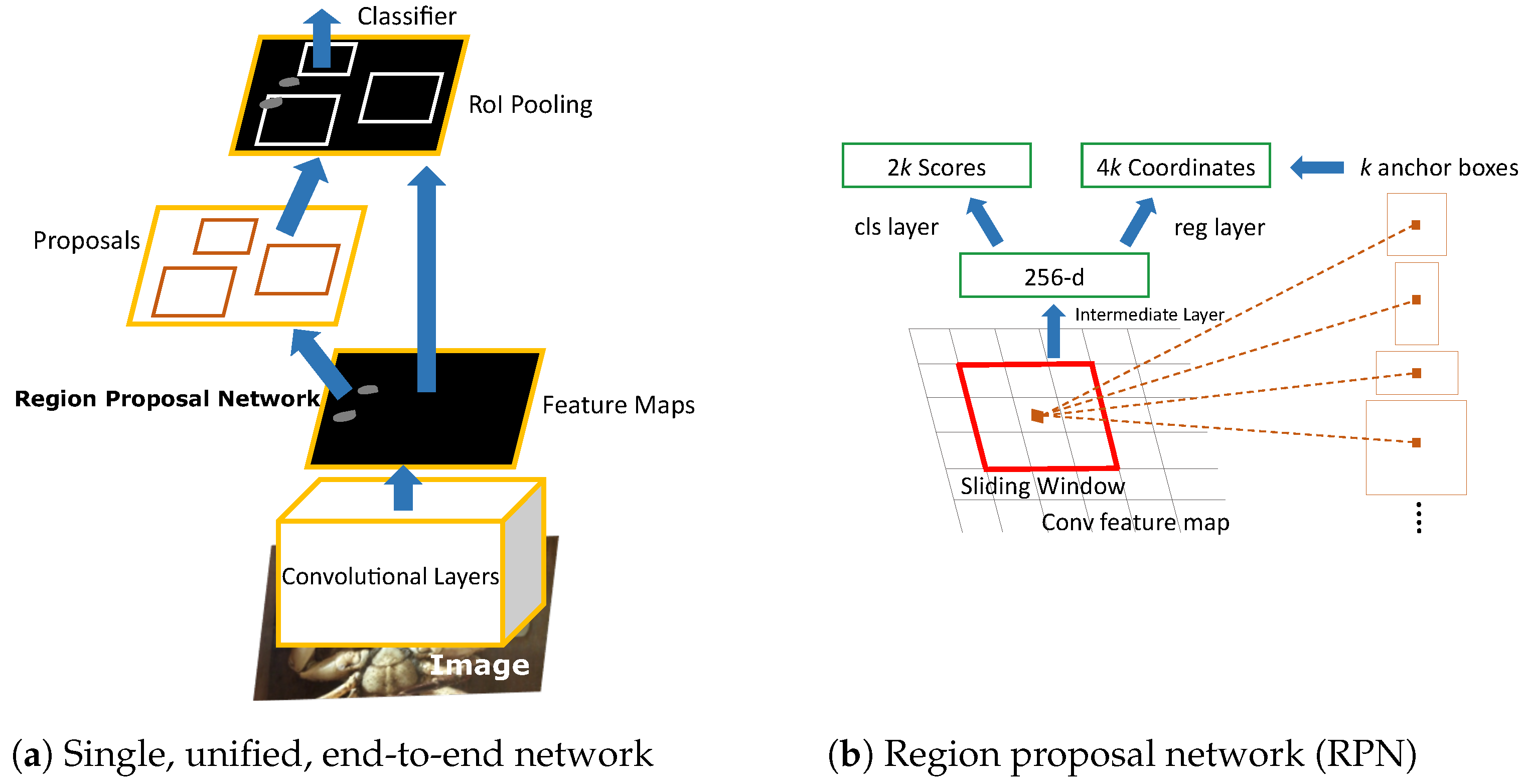
Ren et al. [16] proposed Faster R-CNN with further improvements towards the region-based CNN paradigm. The selective search approach of Fast R-CNN to propose a RoI (Region of Interest) slows down the process, requiring the same time as the detection network. Thus, the region proposal computation is a trade-off between speed and accuracy. Faster R-CNN resolved this by introducing a dedicated fully convolutional region proposal network (RPN) that allows the prediction of region proposals of variant scales and aspect ratios. In addition, the inclusion of RPN boosts the ability to generate region proposals with higher speeds as it shares full-image convolutional features with the detection network and is a step towards near real-time object detection. The RPN runs on a particular conv layer while sharing the previous layers with the object detection network. In order to fully connect to an n × n spatial window, the network slides over the conv feature map depicted in Figure 2b. Each sliding window yields a low-dimensional vector (256, 512), which is fed into the sibling box-classification (cls) and box-regression (reg) layers [41]. The architecture includes n × n and two sibling conv layers with ReLU (Rectified Linear Unit) applied to the n × n conv output layer [41]. In addition to the RPN, anchors are used to detect different-sized objects. Without the requirement for numerous scales of input images or features, the anchors can substantially simplify the process of generating proposals for regions of different sizes. Each region proposal is parametrised relative to a reference anchor box. The distance between the predicted and ground-truth box is estimated to optimise the location of the predicted box. The process of object detection starts with the input image passing through CNN to obtain a set of feature maps. In the next step, the RPN produces bounding boxes and their classification. The selected proposals mapped back to the feature maps obtained from the previous CNN layer in the RoI pooling layer and ultimately fed to the fully connected layer. The result is passed to the classifier and bounding box regressor. The entire process integrates feature extraction, proposal detection, and bounding box regression into a unified, end-to-end learning framework, as depicted in Figure 2a.
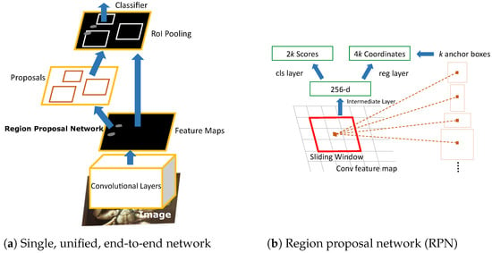
Figure 2.
Faster R-CNN with RPN [16].
For training the RPN, Faster R-CNN keeps the multi-task loss function given in Equation (1).
The loss function calculates probability () and 4k coordinates () for each i-anchor in mini batch, whereas and are the ground-truth label and ground-truth box, respectively. The two terms normalise with , , and the balancing weight . is the Classifier Loss (binary log loss over two classes). is the Regression Loss where , and R is the smooth loss [16].
The bounding box regression parameterises the four coordinates as given in the equation below.
where x, y, w, and h denote the box’s center coordinates and its width and height. Variables x, , and are for the predicted box, anchor box, and ground-truth box, respectively (similarly for y, w, and h) [16].
2.2. You Only Look Once
YOLO [12] was proposed by Joseph Redmon for detecting objects in real-time images and videos. It predicts bounding boxes and class probabilities from input images in a single evaluation. YOLOv3 [14] is an improved version that uses binary cross-entropy loss for the class predictions. It performs the predictions at three different scales. Features are extracted from these scales using a similar concept of FPN to predict the bounding boxes [42]. Several convolutional layers are added to the base feature extractor, and the last layer predicts a 3D tensor encoding bounding box, objectness, and class predictions. YOLOv3 proposed a new network for feature extraction called Darknet-53 that is more efficient than Darknet-19 and the well-known ResNets.
Bochkovskiy et al. [15] proposed YOLOv4 with a higher accuracy and faster operating speed than YOLOv3. The architecture splits into backbone, neck, and head components. The CSPDarknet53 backbone extracts features from the input images. YOLOv4 uses SPP (Spatial Pyramid Pooling) [43] and PAN (Path Aggregation Network) [44] to construct the neck and retains YOLOv3 in the head for predicting the bounding boxes and class probabilities of the input images. Figure 3 depicts the structure of YOLOv4. The mAP increased by 10% compared to that for YOLOv3 (for the MS-COCO dataset) at a real-time speed of 65 FPS on a Tesla V100 GPU. YOLOv4-tiny is a lightweight version of YOLOv4 with fewer convolutional layers, CSPDarknet-tiny backbone, three YOLO layers, and smaller anchor boxes for prediction. It can make faster object detections for running applications on low-power hardware.

Figure 3.
YOLOv4 built with CSPDarknet53, SPP and PAN neck, and YOLOv3 head [15].
2.3. Single-Shot Detector
Liu et al. [45] proposed SSD with the main contribution of introducing multi-reference and multi-resolution detection techniques that have improved the accuracy of one-stage object detectors, mainly on small objects. Having a maximum detection speed of 59 FPS, SSD differs from the other single-stage detectors as it detects different scale objects on multiple network layers, whilst others use the top layer to run detection. It is easy to train SSD and integrate it into other systems as a detection unit. It is claimed that SSD is a high-speed detector due to removing bounding box proposals and the successive feature resampling stage. Also, it uses convolutional filters to recognise object classes and offsets in the bounding box locations. Dedicated predictors are used to perform detection with various aspect ratios and multiple feature maps from the onward stages to detect multiple-scale objects [45]. Figure 4 depicts the SSD framework.

Figure 4.
SSD framework [45].
3. Methods
3.1. Pipeline
We conduct ongoing work on fisheries data collection that covers identification of crabs and lobsters within captured images onboard fishing boats. Our proposed pipeline is made up of multiple steps including (1) finding a video segment with the presence of a crab/lobster; (2) frame selection of individual animals; (3) detecting an animal and drawing a bounding box around it; (4) keypoint detection; and (5) sex identification. This is a novel idea for deployment that can integrate multiple components of data collection like detection, measurement, sexing, counting, etc. It is important to detect the animals in the initial stage followed by extraction of other information on size, sex, and counting of species. The process of detection comes across expected challenges of rotation, occlusion, intra-class variation, illumination, deformation, etc. It is therefore important to explore the strengths and limitations of various detection techniques to conclude the best selection for the problem domain. Multiple object detectors have variant performance in different domains. This paper investigates the performance of distinct object detectors, backbones, and fine-tuned parameters to identify the most optimal solution for detecting crabs and lobsters using our novel dataset.
3.2. Video Capture
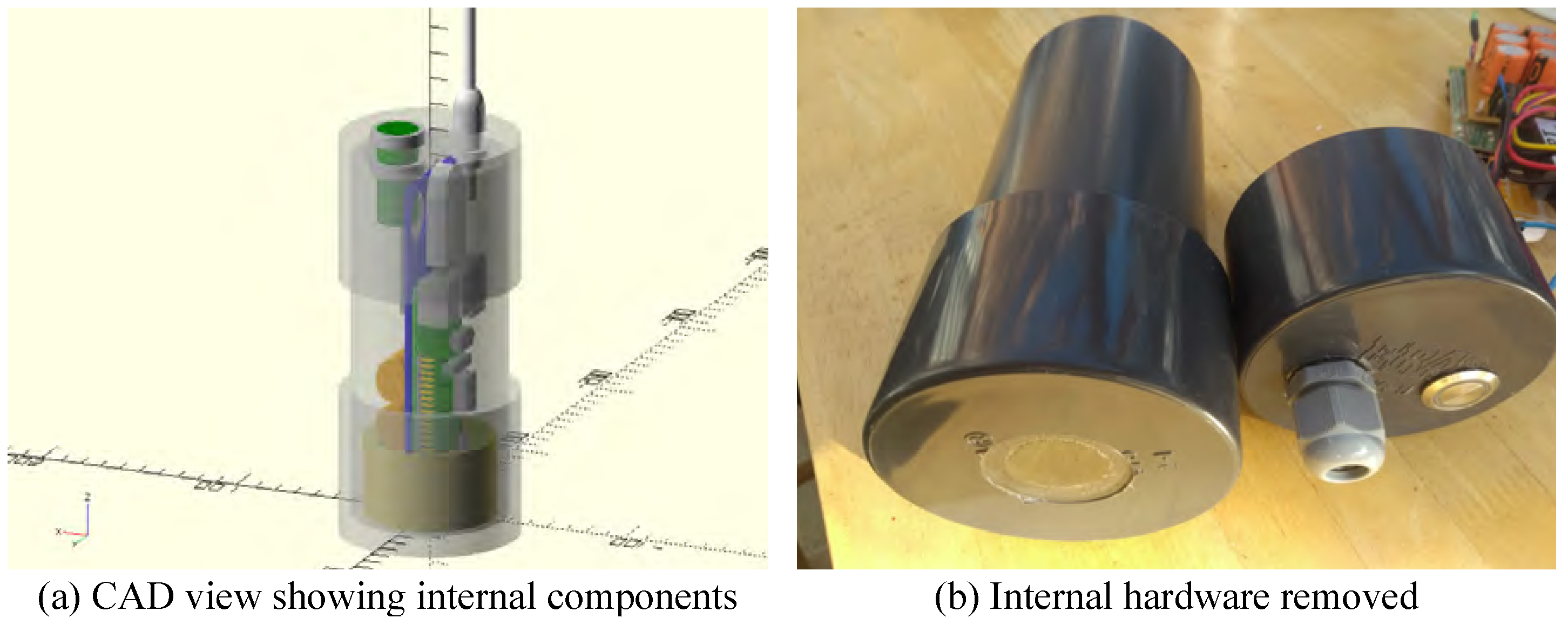
The fishing boats are equipped with camera units aligned on the top of the catch table to record video clips when triggered by motion in the field of view, indicating that something has passed over the catch table. The camera unit (depicted in Figure 5) is a sealed, tough, and waterproof plastic unit, with a 12V DC power supply and a 6 mm clear acrylic window on the bottom surface that captures the video. The high-resolution videos are stored on the camera unit and later downloaded onto WiFi-enabled storage devices.
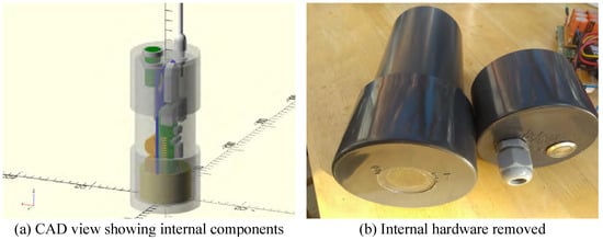
Figure 5.
Sealed waterproof housing with camera. (a) The internal components of the camera have a memory and processing unit. (b) The outer cover shields the camera against water and shocks [10].
3.3. Video Processing and Image Annotation
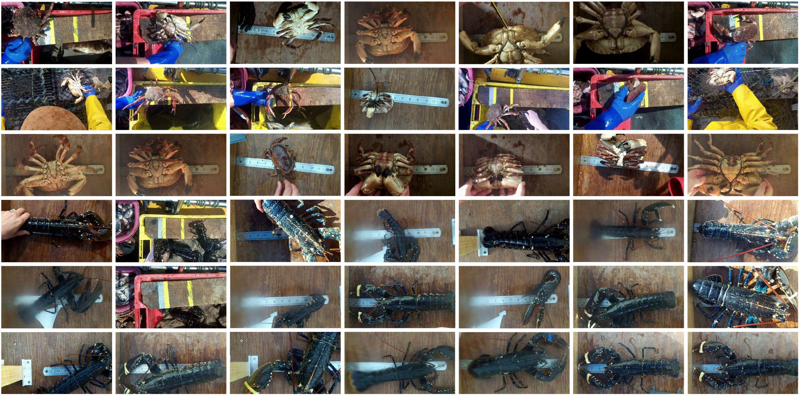
We processed the individual videos for image extraction of crabs or lobsters to train the networks. This is performed by taking the first frame of the video as a reference frame and comparing each image to this. If it is different enough, then the image is stored for processing in the next stage. The difference between images is calculated using a pixel subtraction algorithm, where individual pixels are compared, and if the difference is greater than a set threshold, the image is written to a file and stored in a directory. A new directory of images is created for each set of concurrent frames with a similar threshold. We used 44 videos of different lengths between 5 to 35 min to create our datasets. The main challenges in data collection include dissimilar setups (such as the appearance of the catch tables), highly varied poses of animals, and the presence of unwanted objects in the scene like bycatch, ropes, pots, mud, and gloves. Another problem is the variation in lighting due to moving vessels, outdoor weather conditions, and different times of day during the fishing trips. The selected videos contain crabs and lobsters with different orientations, poses, and sizes. We annotated the images using the LabelImg [46] tool for bounding box positions around the animals and created a dataset of 15,100 images. The dataset was split into 12,080 and 3020 images for the training and test sets, respectively. Figure 6 shows samples from the detection dataset. This novel dataset will allow scientists to extend research on the selected crustaceans.

Figure 6.
Sample images from the crab and lobster detection dataset.
3.4. System Configuration and Evaluation
We performed the training and evaluation of the networks using a Geforce RTX 3070 (16 GB) GPU, 32 GB memory, Core i7 CPU, CUDA toolkit 11.4.0, cuDNN 8.5.2, tensorflow-gpu 2.5.0, tensorboard 2.10.0, OpenCV 4.5.4.60, Python 3.9.0, and other libraries. We will use the results achieved on this hardware to inform the design and specification of future deployment hardware.
We assessed the performance of the trained models using mAP, IoU, F1 score, and recall, calculated by Equations (3)–(7) below.
The evaluation relies on TP (true-positive), TN (true-negative), FP (false-positive), and FN (false-negative) predictions. IoU is the intersection of the predicted and the actual bounding boxes divided by their union. A prediction is a true positive if IoU > the set threshold and a false positive if IoU < the threshold. The mean average precision is an evaluation metric for object detection. Each bounding box will have a score associated with it. Based on the predictions, a precision-recall curve (PR curve) is computed for each class by varying the score threshold. The average precision (AP) is the area under the PR curve. The AP for each class is computed and then averaged over the total number of classes.
4. Experiments and Results
4.1. Faster R-CNN, SSD, and Lightweight MobileNets
We trained Faster R-CNN and SSD on three different backbones i-e Inception v2, ResNet-50 (v1), and ResNet-101 (v1). The inclusion of SSD lightweight networks aims to provide a solution for low-power hardware. The lightweight networks were built of SSD with MobileNetV1, MobileNetV2, MobileNetV3, SSDLite MobileNetV1, and SSDLite MobileNetV2. SSD and MobileNets train faster models for detecting objects in images. The fine-tuned parameters were configured at learning rate (0.0002), momentum optimiser (0.9), grid anchor values (0.25, 0.5, 1.0, and 2.0), aspect ratios (0.5, 1.0, and 2.0), batch size (1), and 50k training steps. We used tensorboard to visualise the training and evaluation graphs. We automated checkpoints at 5k steps to generate the inference graphs and saved the models. The experiments are performed on a dataset of 15,100 images, with training and testing splits of 12,080 and 3020 images, respectively. We conducted trainings with three different input sizes of , , and .
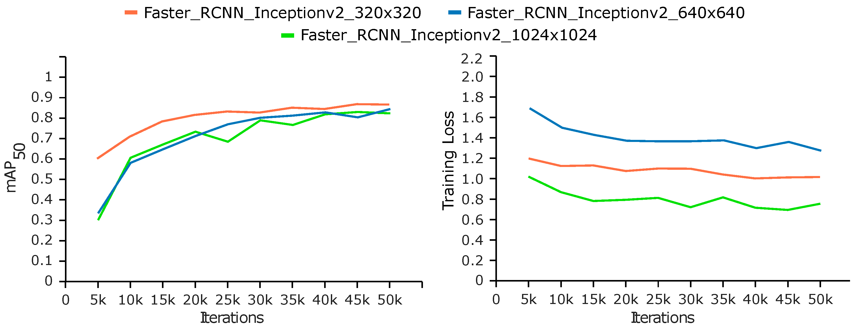
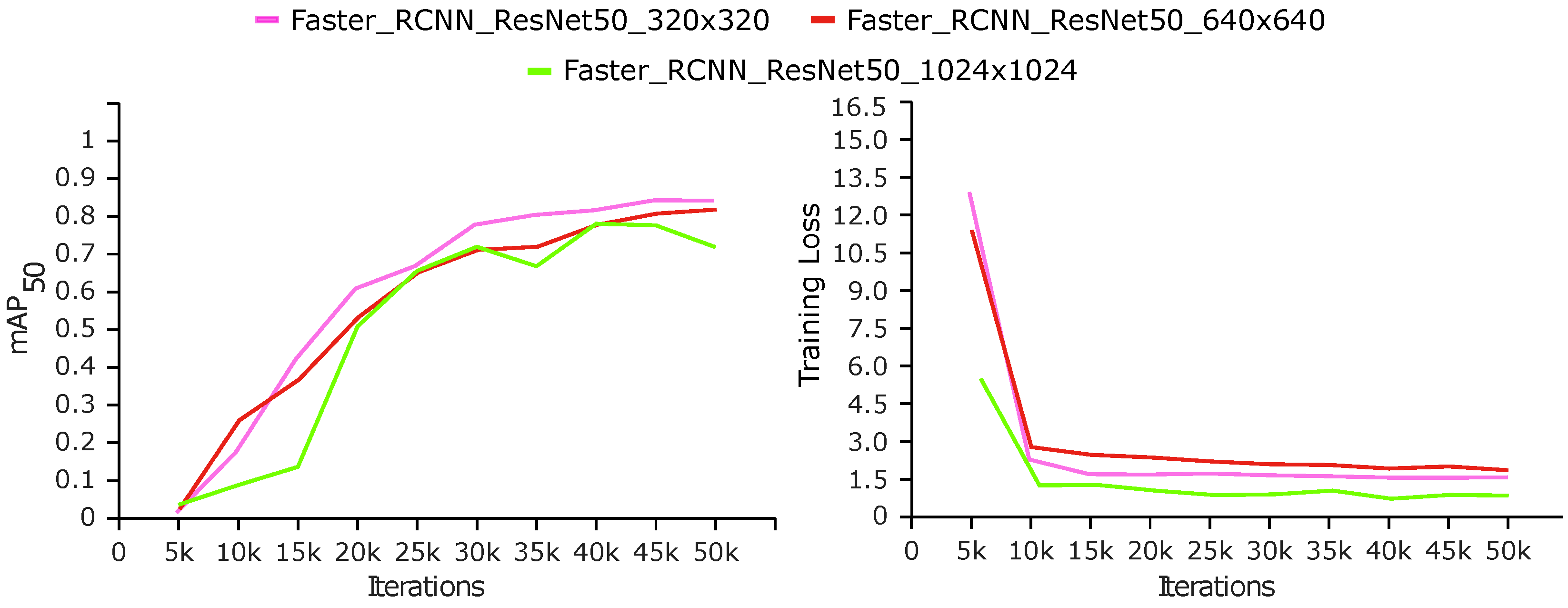
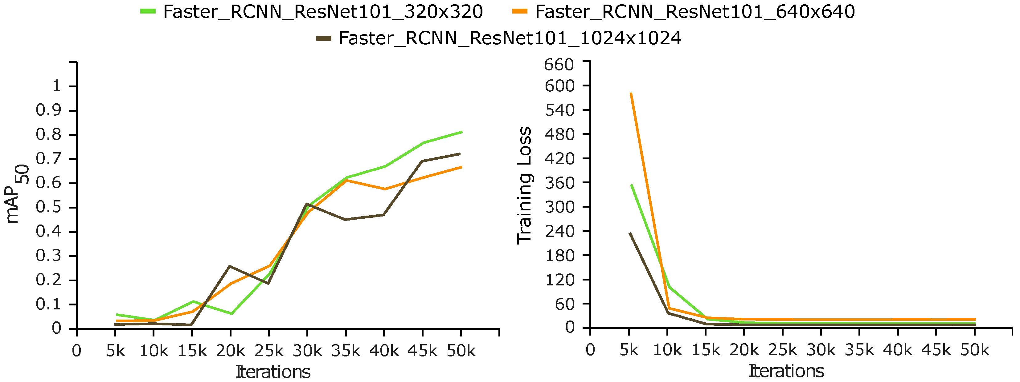
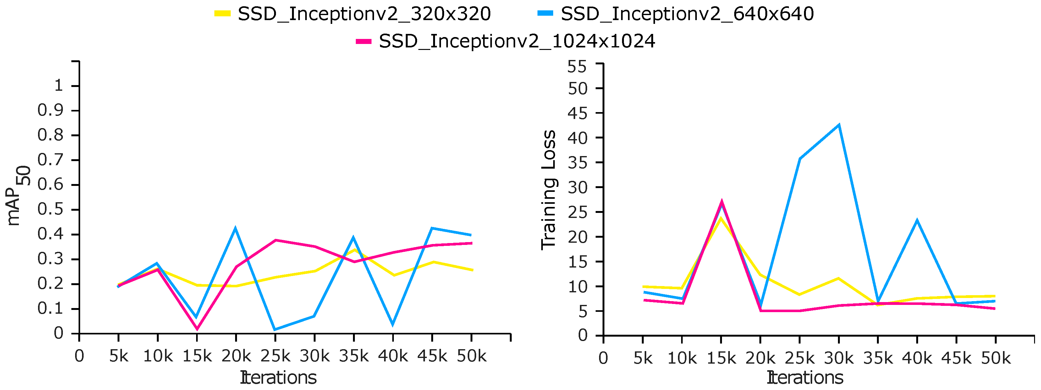
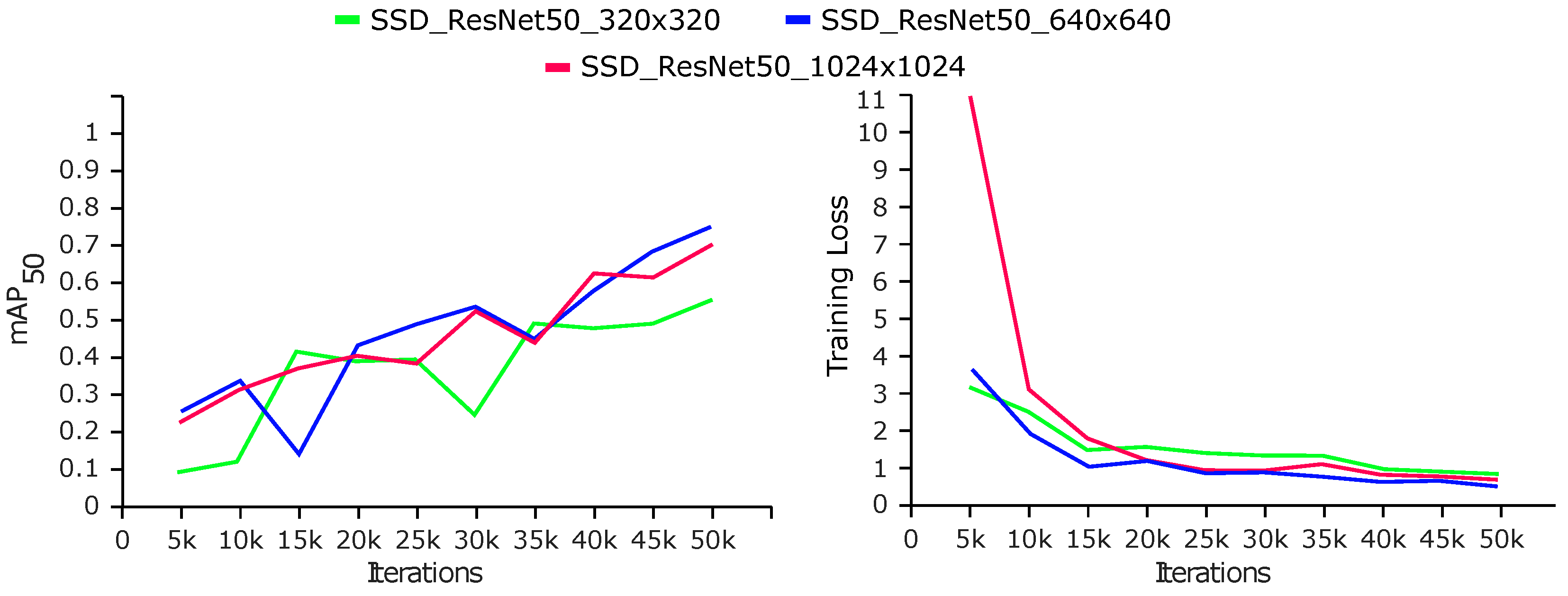
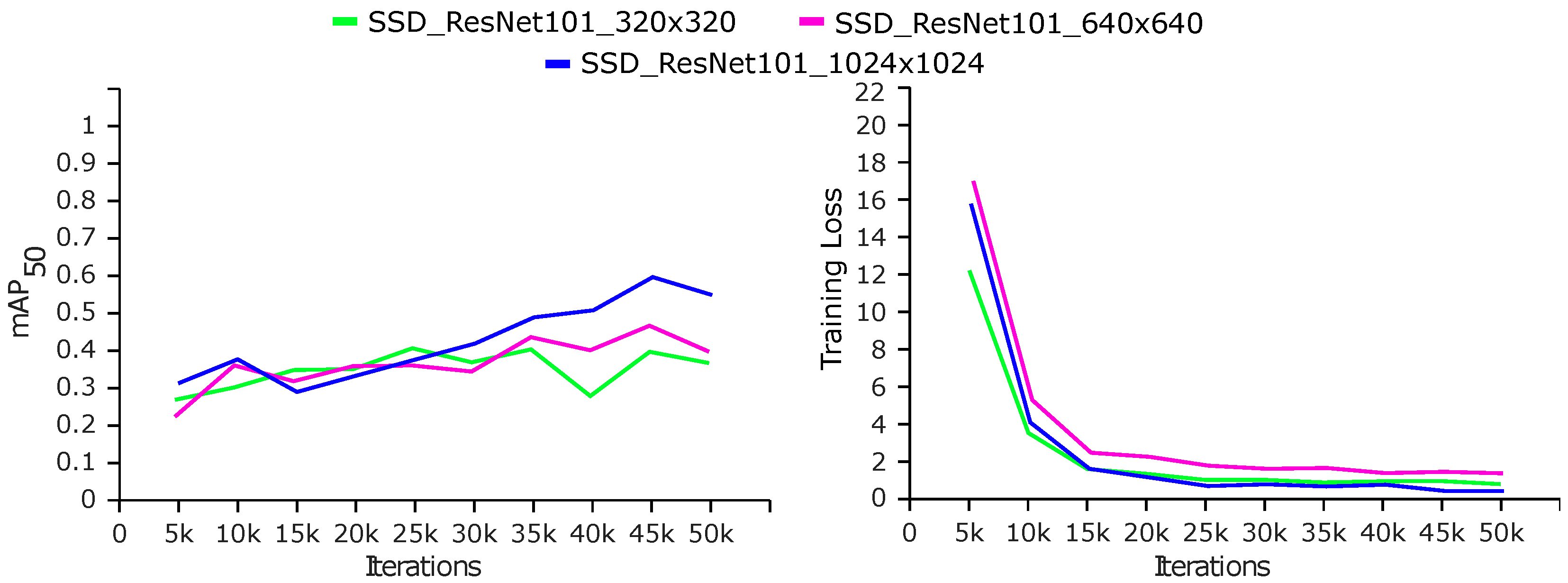
We evaluated the results using mAP, recall, and F1 score. The FPS estimates the response time of the trained model. Faster R-CNN achieved a maximum mAP of 88.8%, 87.1%, and 80.4% with Inception v2, ResNet-50, and ResNet-101, respectively. The FPS for a lower input size remained high and vice versa. The FPS values varied between 3 and 12 for different trials. The selection of a low input size reduced the training time and vice versa. SSD achieved maximum mAP values of 56.8%, 75.7%, and 64.3% for the three backbones, respectively, which were lower by 32%, 11.4%, and 16.1% than Faster R-CNN. SSD ResNet-50 achieved the highest recall of 75.7%, the lowest training loss of 0.6, and a higher FPS than Faster R-CNN. Inception v2 trained faster than ResNet-50 followed by ResNet-101. Table 2 and Table 3 present the results of Faster R-CNN and SSD, respectively. Figure 7, Figure 8 and Figure 9 and Figure 10, Figure 11 and Figure 12 show the comparison of Faster R-CNN with SSD, respectively.

Table 2.
Results of Faster R-CNN evaluated on a test set of 3020 images. The best results in the column are formatted as red bold.

Table 3.
Results of SSD evaluated on a test set of 3020 images. The best results in the column are formatted as red bold.
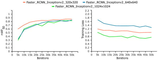
Figure 7.
Performance analysis of Faster R-CNN Inception v2 on a test set of 3020 images and input sizes of , , and .

Figure 8.
Performance analysis of Faster R-CNN ResNet-50 on a test set of 3020 images and input sizes of , , and .
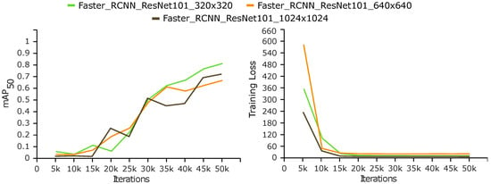
Figure 9.
Performance analysis of Faster R-CNN ResNet-101 on a test set of 3020 images and input sizes of , , and .
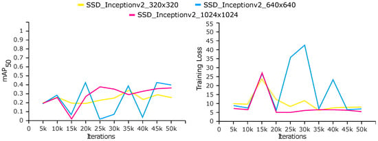
Figure 10.
Performance analysis of SSD Inception v2 on test set of 3020 images and input sizes of , , and .
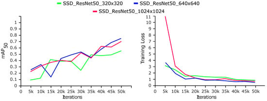
Figure 11.
Performance analysis of SSD ResNet-50 on a test set of 3020 images and input sizes of , , and .
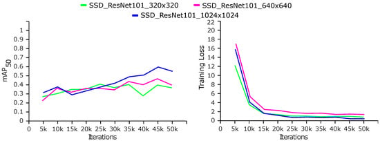
Figure 12.
Performance analysis of SSD ResNet-101 on a test set of 3020 images and input sizes of , , and .
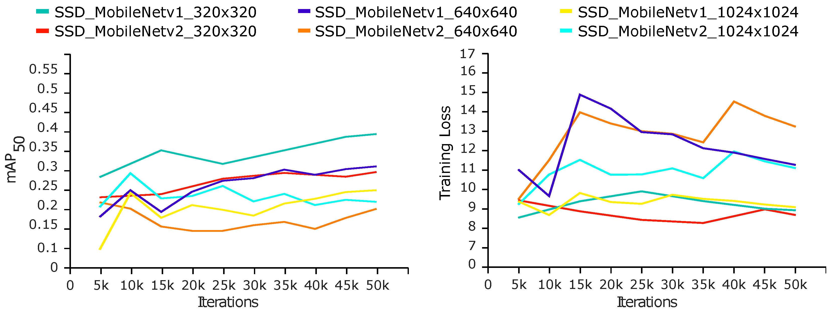
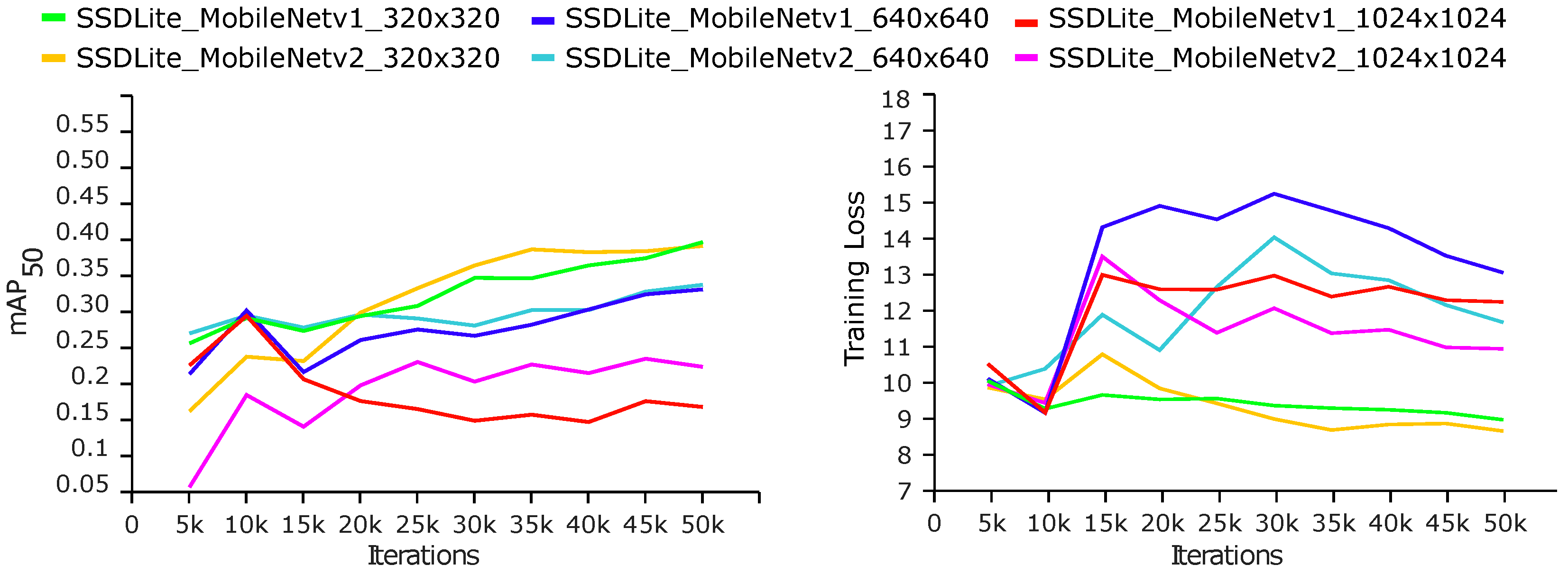
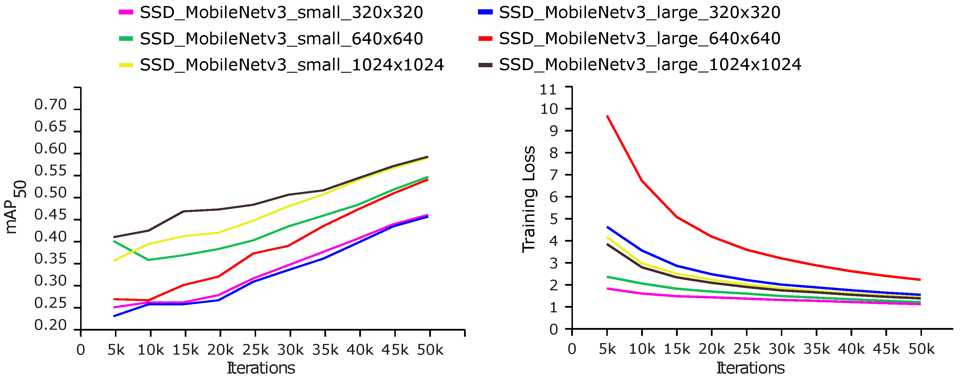
We trained SSD with three different versions of lightweight MobileNet for 50k steps. The results show that SSD trained on lightweight MobileNets produces a higher FPS than ResNets and Inception v2. The input size of did not effectively improve the mAP and decreased in some cases (S.No. 2, 3, 8, 9, and 12 of Table 4). The mAP, recall, and F1 scores decreased compared to base models but achieved higher FPS rates up to 47 with SSD MobileNet V3-Small calculated on an Nvidia GTX 1650 GPU. SSDs are faster but less accurate than Faster R-CNN. The precision of the models in S.No. 1–12 of Table 4 is around 50%, whereas the results of SSD MobileNetV3 (both the Small and Large versions) had improved mAP and FPS to 84.8% and 47, respectively. Figure 13, Figure 14 and Figure 15 depict the results of SSD MobileNets. Figure 16 depicts the qualitative analysis of the models discussed above.

Table 4.
Results of SSD and SSDLite with MobileNets on a test set of 3020 images and input sizes of , , and . The best results in the column are formatted as red bold.
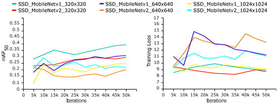
Figure 13.
Performance analysis of SSD MobileNet V1, V2 on test set of 3020 images and input sizes of , , and .

Figure 14.
Performance analysis of SSDLite MobileNet V1 and V2 on a test set of 3020 images and input sizes of , , and .
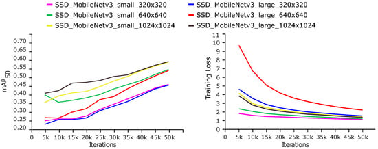
Figure 15.
Performance analysis of SSD MobileNetV3 (small and large) on a test set of 3020 images and input sizes of , , and .
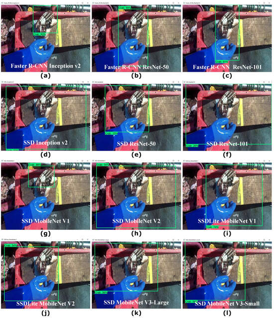
Figure 16.
Qualitative analysis of Faster R-CNN, SSD, and lightweight models on a sample image trained for crab and lobster object detection. Left to right: (a–l) Faster R-CNN Inception v2, Faster R-CNN ResNet-50, Faster R-CNN ResNet-101, SSD Inception v2, SSD ResNet-50, SSD ResNet-101, SSD MobileNetV1, SSD MobileNetV2, SSDLite MobileNetV1, SSDLite MobileNetV2, SSD MobileNetV3-Large, and SSD MobileNetV3-Small.
4.2. Object Detection with YOLO (v3, v4)
We trained YOLOv3 and YOLOv4 using the Darknet53 backbone and the 15.1k dataset with 12,080 and 3020 images in the training and test sets, respectively. We trained YOLO (v3, v4) with input sizes of , , and , a momentum value of 0.9, a decay of 0.0005, and a learning rate of 0.001 for a maximum of 6000 training iterations.
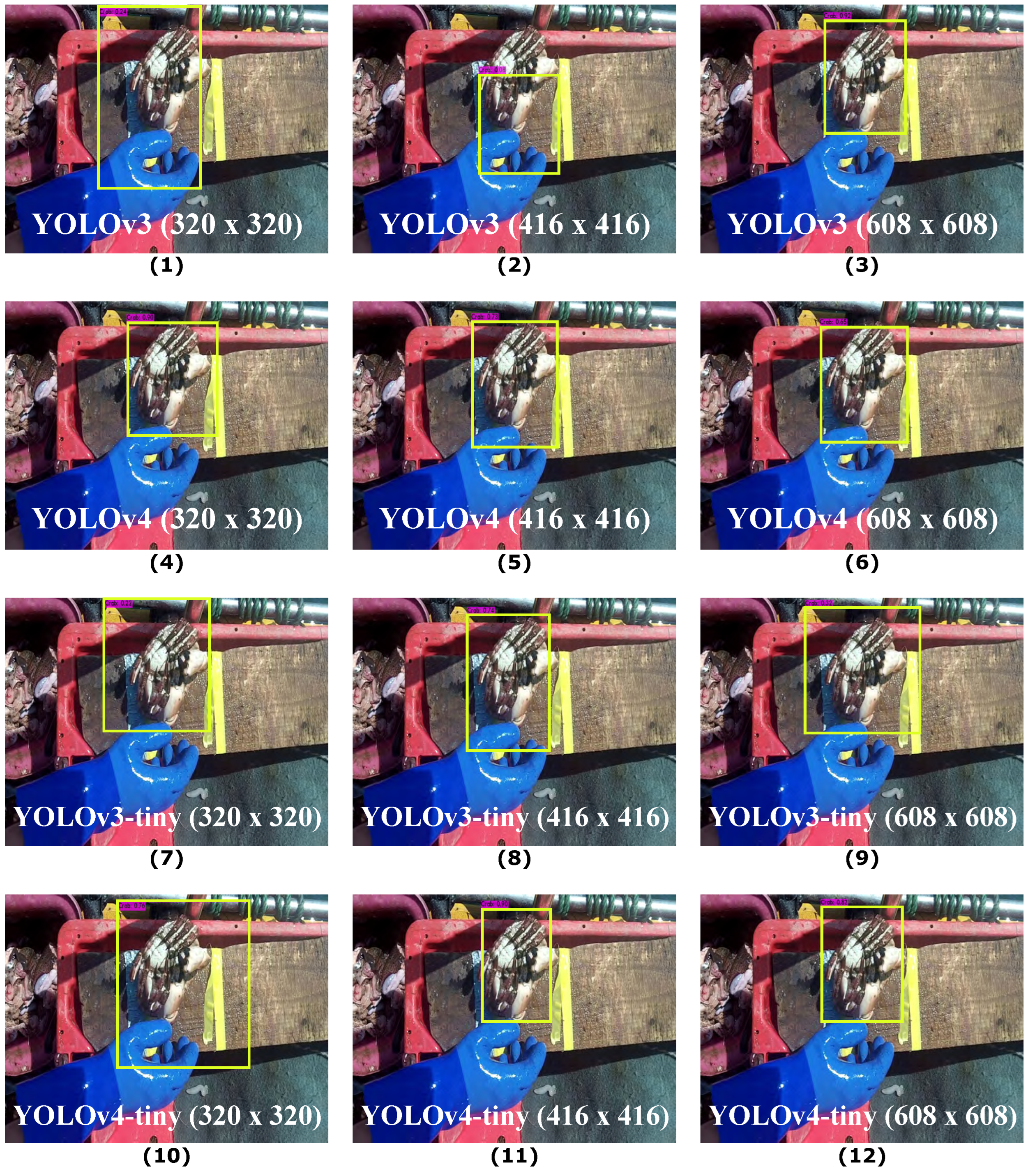
The results obtained are given in Table 5. The results improved with increasing input size. YOLOv4 achieved improved results with a maximum mAP of 97.5%, which is 10.2% higher than YOLOv3. The FPS remained the same for both the YOLO base models. The average loss was less than 1 in all experiments. We also trained the tiny lightweight versions of YOLO (v3, v4) which are faster with a lower mAP. The YOLOv4-tiny achieved a maximum mAP of 85.4%, which is 12.1% less than the base model. However, the tiny versions support low-power hardware with a faster speed of 64 FPS. Figure 17 depicts the qualitative analysis of YOLO with default anchors.

Table 5.
Results of YOLO and YOLO-tiny on a test set of 3020 images and input sizes of , , and . The best results in the column are formatted as red bold.
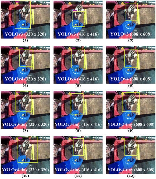
Figure 17.
Qualitative analysis of YOLO with default anchors (1–12 of Table 5) on a sample image.
4.3. Comparison of YOLO (v3, v4) and Tiny Models
A trade-off exists between speed and accuracy among different variants of YOLO. The networks differ in the number of layers and trainable parameters, which is reflected in the training and inference times of the models. The FPS, BFLOPS, and weight size are other indicators for measuring the speed of the networks. Larger networks are mostly expensive and require high memory and processing power to train and operate.
YOLOv3 is based on Darknet-53 and is built of 106 layers including 53 convolutional and 3 YOLO layers (positioned at 82, 94, and 106) for detection. The network has 62 M trainable parameters, an inference speed of 50 ms, and a weight size of 235 MB. YOLOv3-tiny has a lighter structure of 24 layers in total having 13 convolutional and 2 YOLO layers. The number of trainable parameters is reduced to 8.7 M, the inference time is 8.3 ms, and the weight size is 33 MB, which accelerates the speed of the network compared to YOLOv3.
YOLOv4 is structured with 162 layers having 53 convolution layers and each convolution layer connects with a batch normalisation and Mish activation layer. It includes 3 YOLO layers (positioned at 139,150,161) for detection. The total number of trainable parameters is 64.4 M, the weight size is 244 MB, and the inference time is 45.8 ms. The YOLOv4-tiny architecture consists of 38 layers including 21 convolutional layers and 2 YOLO layers. It is faster than YOLOv4 having 6.8 M trainable parameters, a weight size of 22 MB, and an inference time of 8.3 ms.
The tiny variants make the training process faster with fewer computations with some trade-off in detection performance. Table 6 shows the comparison of the size and speed of the YOLO networks.

Table 6.
Structure and speed comparison of the YOLO (v3 & v4) and tiny models.
5. Optimised Benchmark YOLOv3, YOLOv4, and Tiny Versions
YOLO predicts bounding boxes and class probabilities from input images in a single evaluation. YOLOv3 uses binary cross-entropy loss for class predictions and performs the predictions at three different scales. Features are extracted from these scales using a similar concept of FPN to predict the bounding boxes. Several convolutional layers are added to the base feature extractor, and the last layer predicts a 3D tensor encoding bounding box, objectness, and class predictions. YOLOv3 uses Darknet-53 for feature extraction with 53 convolutional layers and is better than Darknet-19. YOLOv4 improved YOLOv3 with a CSPDarknet53 backbone for feature extraction.
YOLO divides each input image into multiple grids that help in identifying objects. Each grid cell predicts multiple bounding boxes along with their corresponding class probabilities. YOLO utilises multiple anchors for each grid cell to support object classes of different shapes and sizes. YOLOv3 uses the pre-defined anchor boxes proposed in [14] with three scales associated with a specific feature map to detect objects at various scales. The scale 1 anchors are associated with a feature map representing the largest respective field. The scale ratios for this anchor set are (116, 90), (156, 198), and (373, 326). The scale 2 anchors are associated with a feature map with scale ratios of (30, 61), (62, 45), and (59, 119), and the scale ratios for the third scale of anchors associated with a feature map are (10, 13), (16, 30), and (33, 23). Thus, each scale has three anchor boxes associated with it. The number of anchor boxes is fixed and independent of the number of classes detected, and YOLOv3 predicts three bounding boxes per grid cell. The entire set of anchors of the three scales is {10,13, 16,30, 33,23, 30,61, 62,45, 59,119, 116,90, 156,198, 373,326}. Similarly, the set of default anchors for YOLOv4 is {12,16, 19,36, 40,28, 36,75, 76,55, 72,146, 142,110, 192,243, 459,401}.
The tiny versions of YOLOv3 and YOLOv4 use anchors to predict object locations and sizes in images. However, the configurations of the anchors differ for the tiny variants of YOLO. They are simpler in design than the baseline YOLO models aiming to achieve a balanced speed and accuracy for real-time resource-constrained applications. The default anchor set for YOLO-tiny (v3 and v4) is represented as {10,14, 23,27, 37,58, 81,82, 135,169, 344,319}.
K-Means Clustering
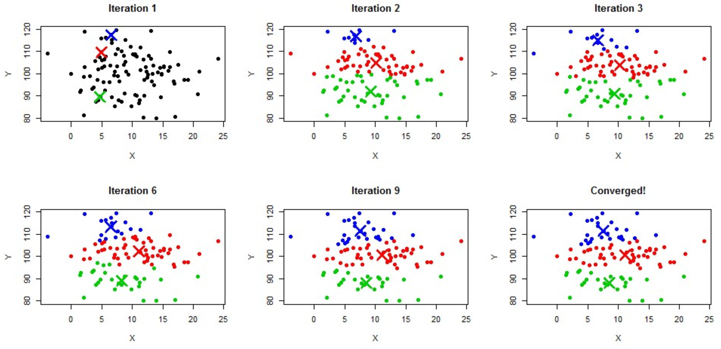
The k-means clustering algorithm [47] is an unsupervised learning algorithm used to solve the clustering problems in ML. It can predict similar data points together, using a fixed number k of clusters in the dataset. The k-means algorithm finds k centroids, keeps the centroids as small as feasible, and then assigns each data point to the closest cluster. The k defines the number of pre-defined clusters that need to be created in the process; thus, if k = n, then there will be n clusters. It first determines the best value for k centre points or centroids by an iterative process and then assigns each data point to its closest k-centre. Finally, the data points closer to the particular k-centre create a cluster. Figure 18 depicts the steps of cluster convergence by the k-means algorithm.
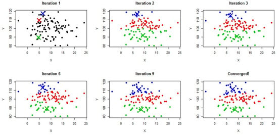
Figure 18.
k-means clustering of data points with three randomly initiated centroids represented by blue, red and green colours [48].
Custom Anchor-Based YOLO Experiments and Results
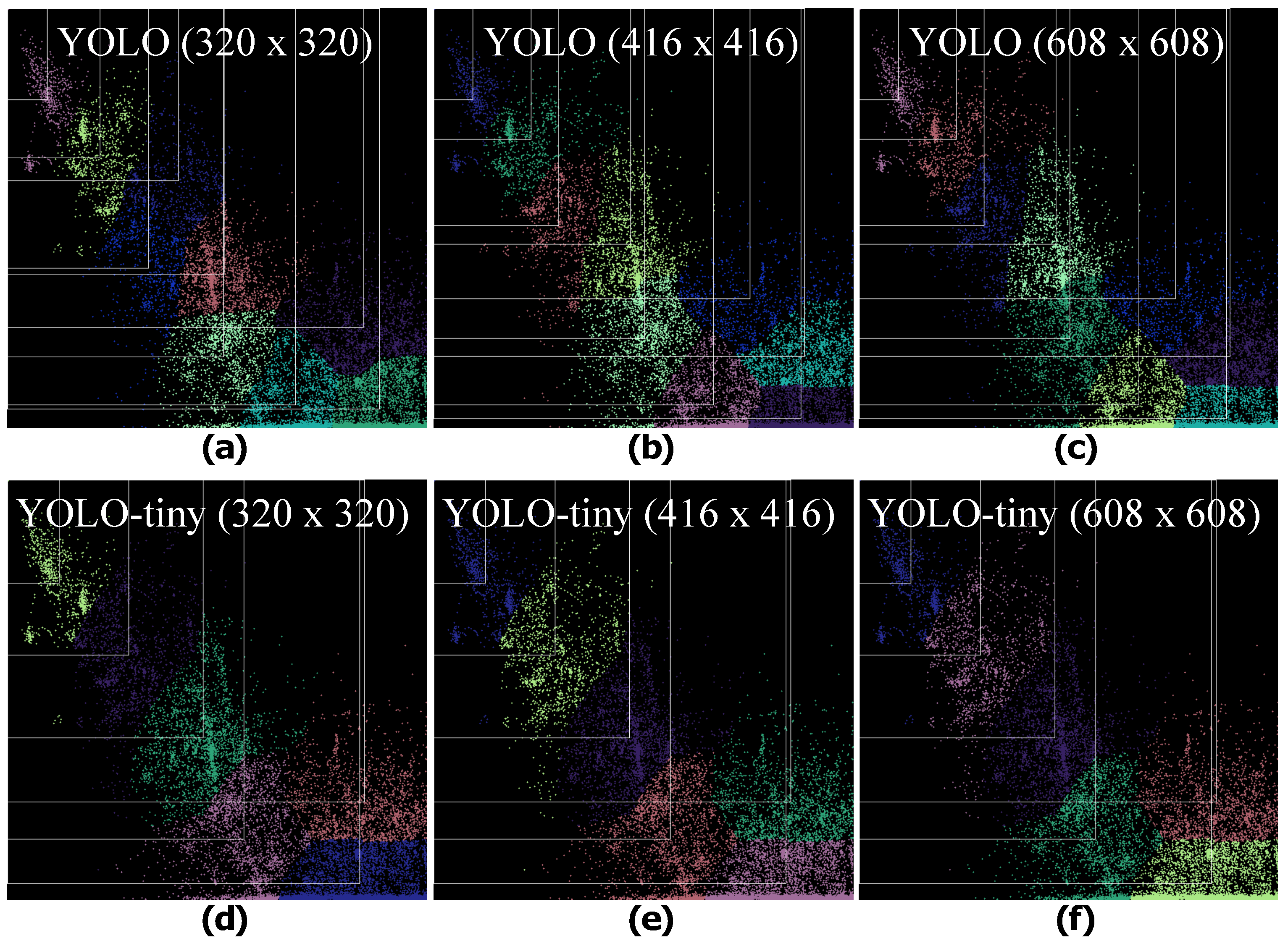
YOLO depends on set of anchors to predict bounding boxes in images. The precise configuration of anchors improves the training of object detectors to achieve better results. We applied k-means clustering algorithm to generates anchors for YOLO using 12,080 images of the train set of our dataset for input sizes of , , and . The base and tiny models of YOLO use 9 and 6 pairs of anchors, respectively using the same number of clusters to generate them. Table 7 shows the detail of anchors generated for YOLO (v3, v4) and their tiny variants. Figure 19 depicts the converged clusters and anchor boxes for the input sizes of , , and . We trained the YOLO (v3 and v4) configured for new anchor sets to detect crabs and lobsters. Table 8 shows the results.

Table 7.
Anchor calculation using k-means clustering on a training set of 12,080 images. The YOLO base and tiny models are trained on a set of 9 and 6 pairs of anchors, respectively, for three input sizes.
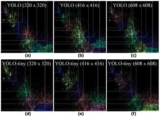
Figure 19.
Visualisation of the clusters based on three different input sizes for YOLO base models (a–c) and tiny models (d–f).

Table 8.
Results of the improved YOLOv3, YOLOv4, YOLOv3-tiny, and YOLOv4-tiny models with custom anchors on a test set of 3020 images [ca=custom anchors]. The best results in the column are formatted as red bold.
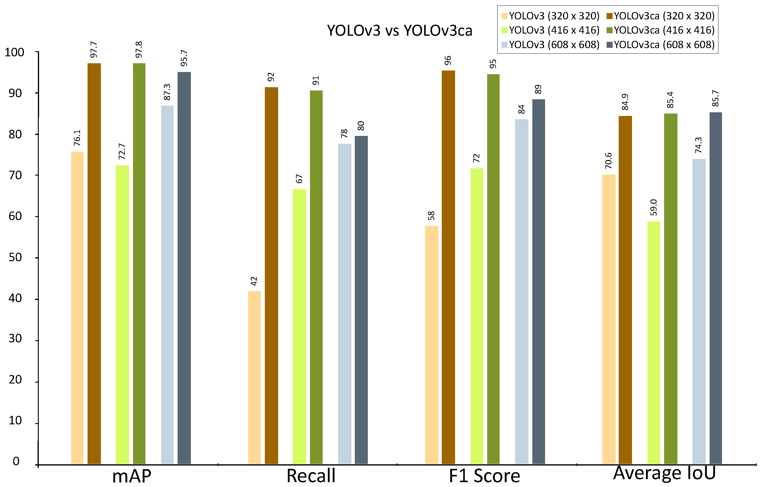
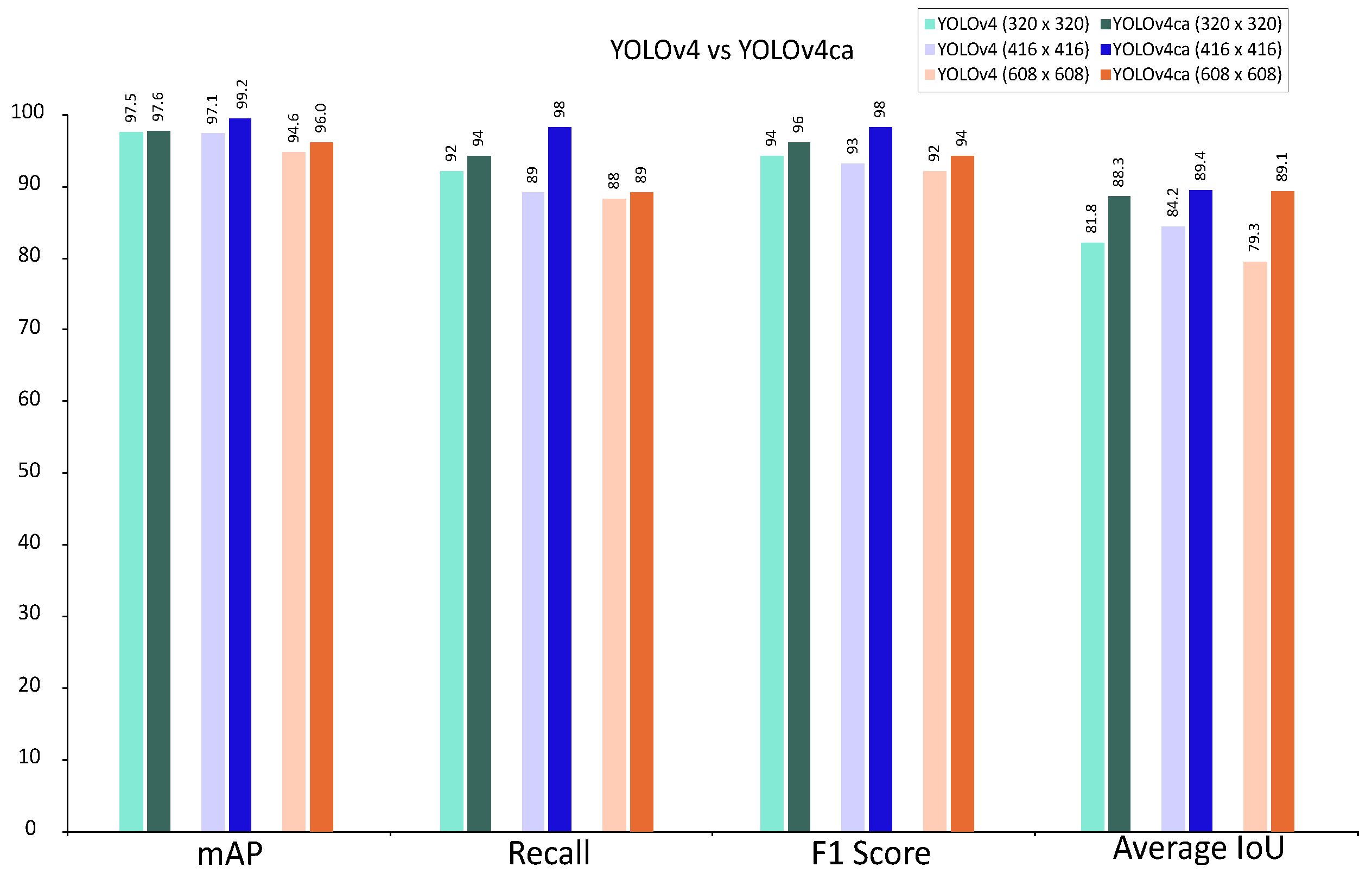
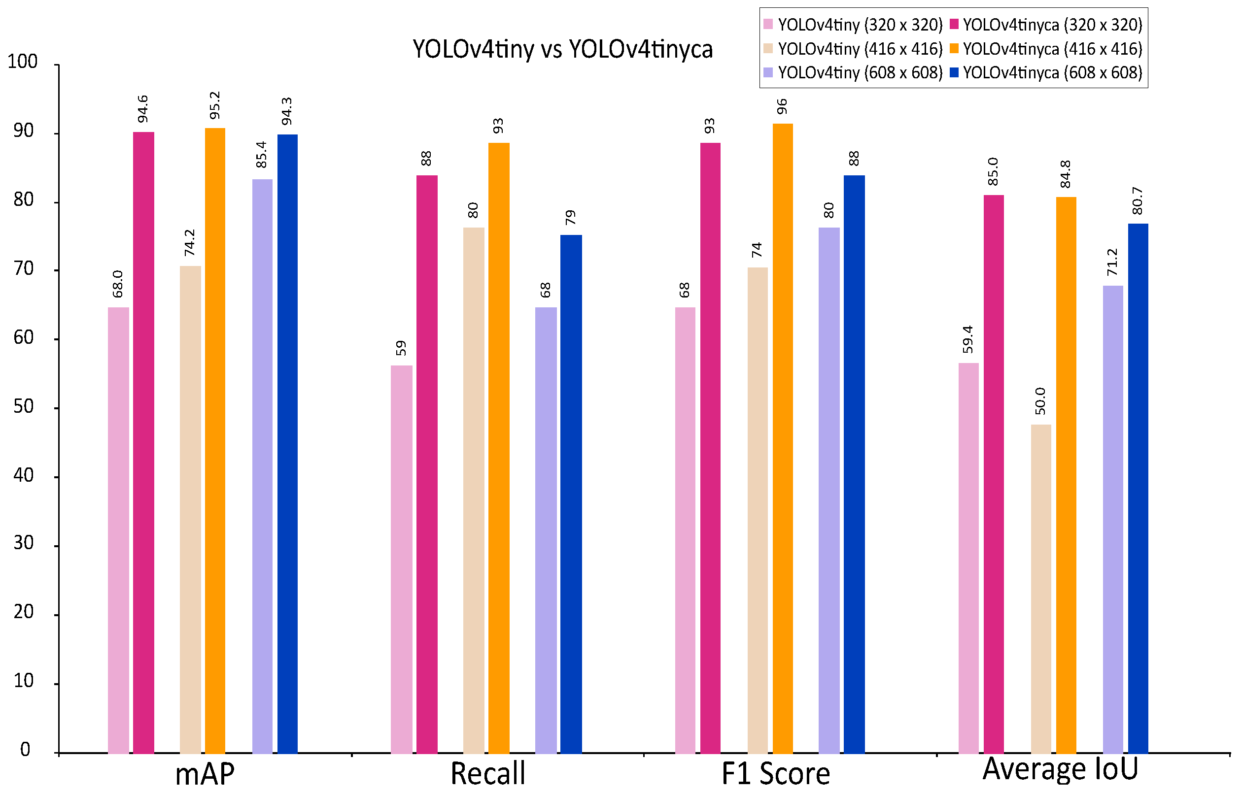
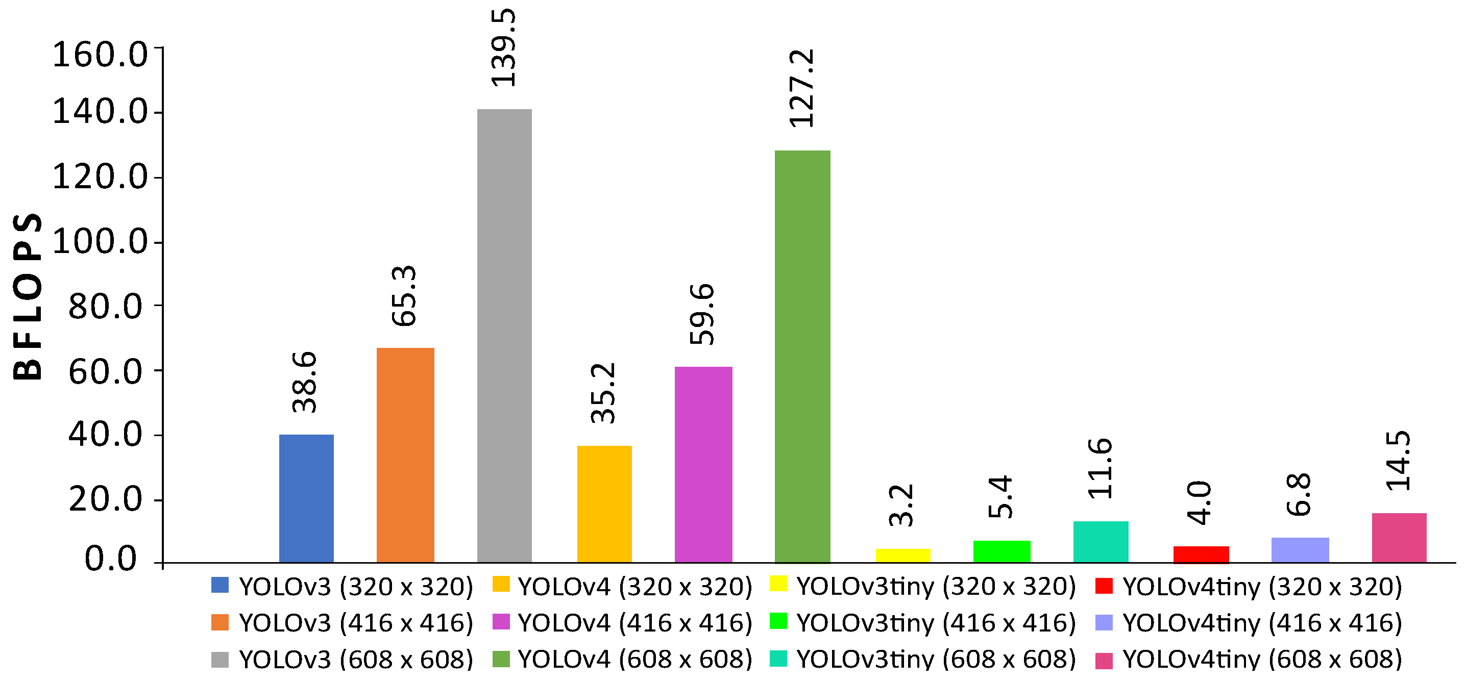
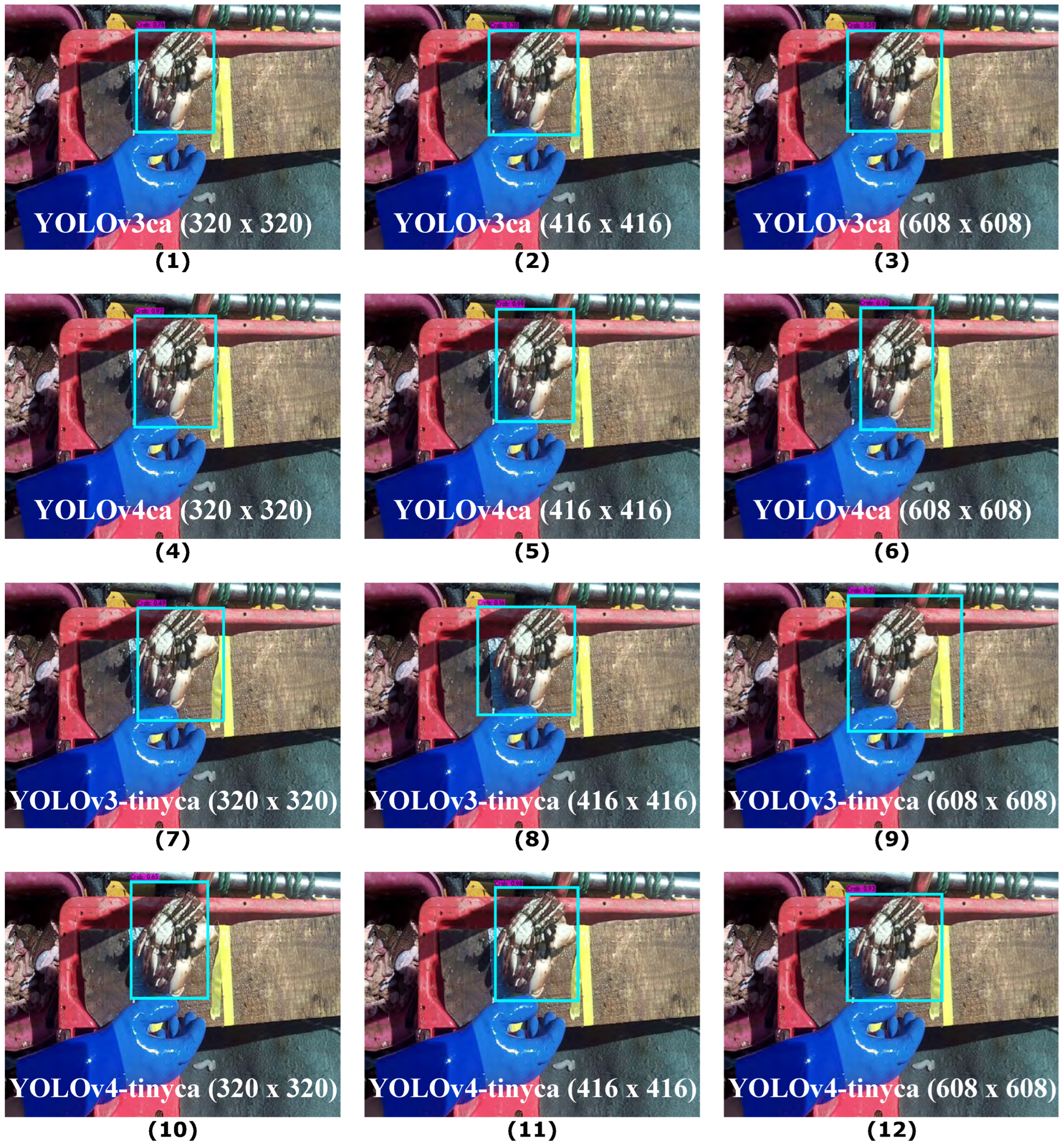
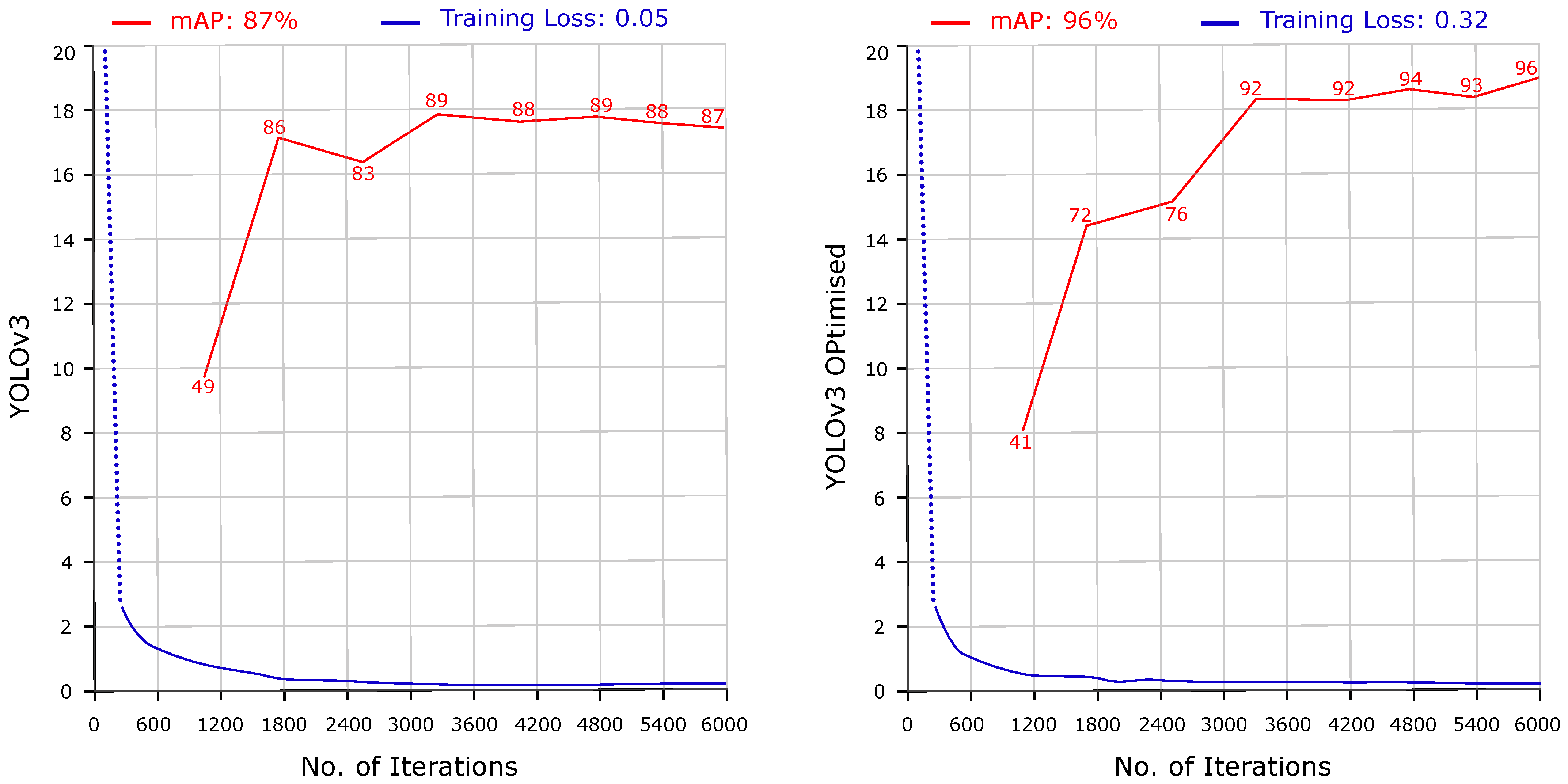
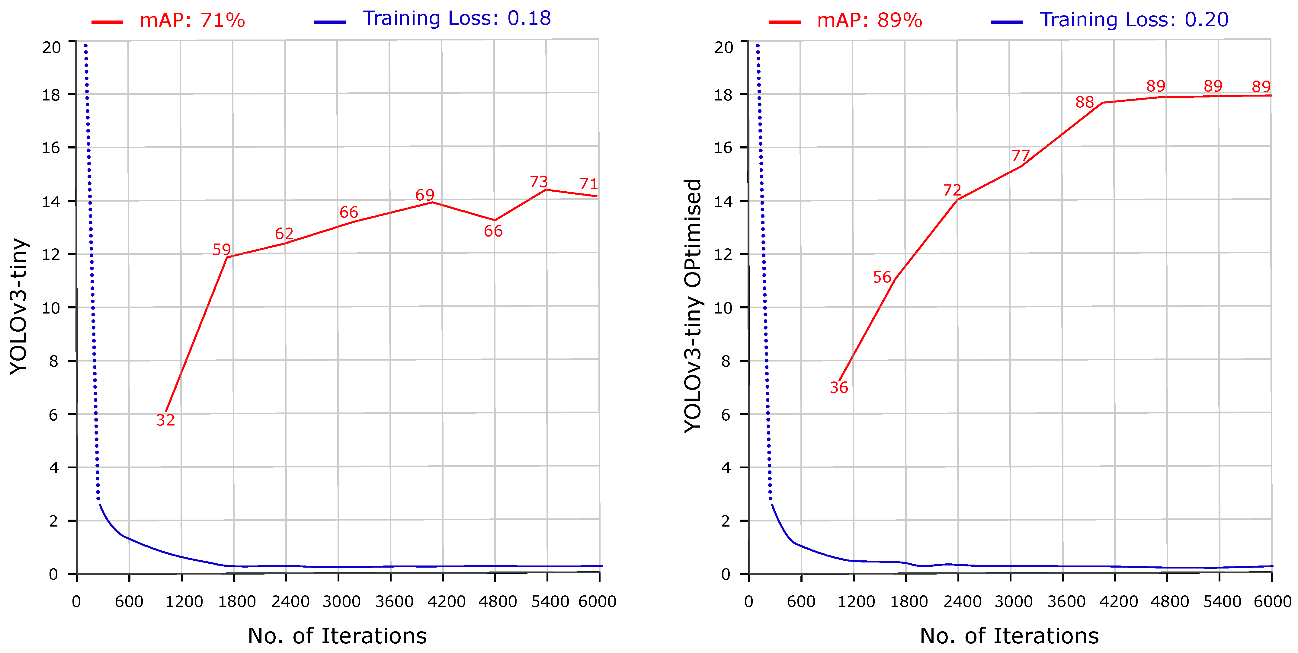
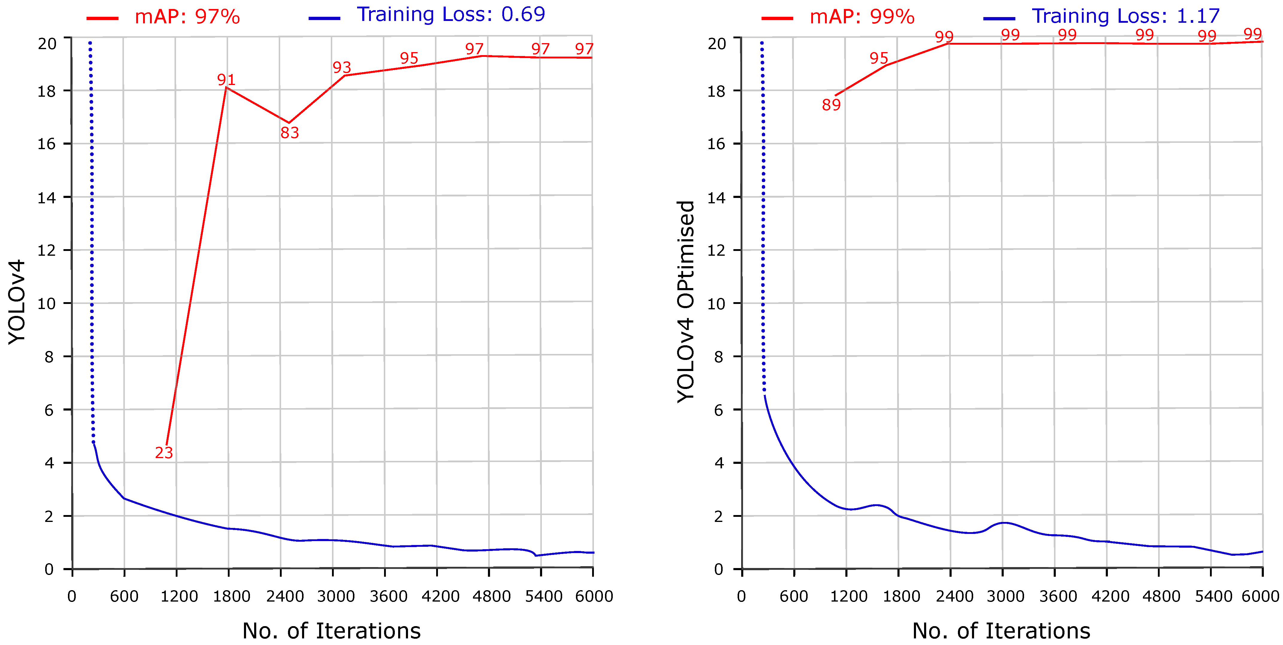
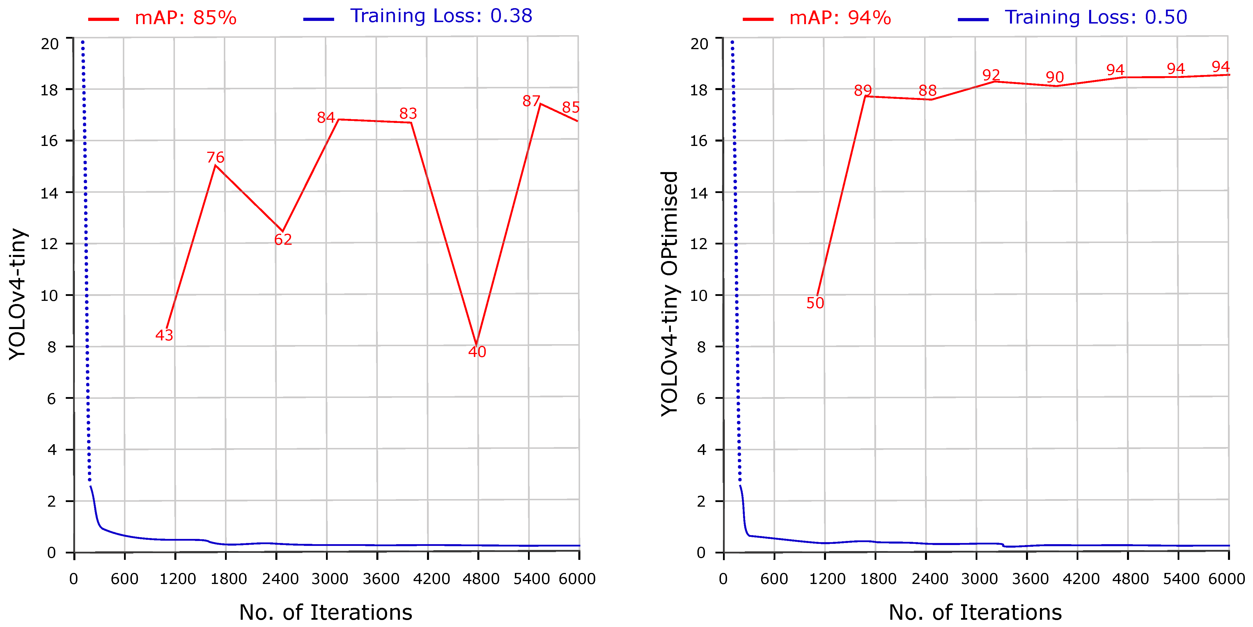
The anchors generated for our dataset images improved the results of the YOLO detectors. We trained the object detectors on 12,080 images and evaluated the results on 3020 images. We selected three input sizes of , , and . The mAP of YOLOv3 improved by 21.6%, 25.1%, and 8.4% for , , and , respectively, compared to using the default anchors. The mAP of YOLOv4 improved by 0.1%, 2.1%, and 1.4% for the three input sizes, respectively. The results of the tiny versions show significant improvement with the custom anchor-based training on the custom dataset. The mAP of YOLOv3-tiny improved by 18.2%, 14.2%, and 8.3% for the three input sizes, respectively. The mAP of YOLOv4-tiny increased by 26.6%, 21%, and 8.9% for the input sizes of , , and , respectively. The results improved compared to Table 5 above. We trained models with a highest mAP of 99.2% and 95.2% for YOLOv4 and it’s tiny version, respectively. Figure 20, Figure 21, Figure 22 and Figure 23 depict the results (mAP, recall, F1 score, and average IoU) of the trained object detectors. The training loss remained less than 1 for the total 6000 training iterations. The tiny models are faster than the base models with an FPS of 64 and BFLOPS between 3.2 to 14.5. The maximum FPS for the base models was 32. Figure 24 depicts a comparison of BFLOPS. Table 8 shows the list of results obtained. Figure 25 presents the qualitative analysis of the results for a sample image. Figure 26, Figure 27, Figure 28 and Figure 29 visualises the training loss and mAP of the trained models.
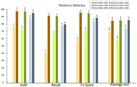
Figure 20.
Comparison of mAP, recall, F1 score, and average IoU of the YOLOv3 and YOLOv3ca models. Dark coloured bars represent the optimised results.
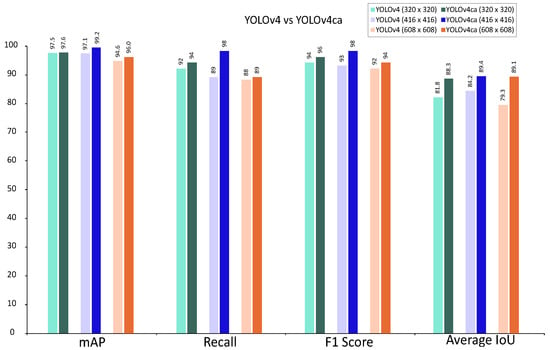
Figure 21.
Comparison of mAP, recall, F1 score, and average IoU of the YOLOv4 and YOLOv4ca models. Dark coloured bars represent the optimised results.
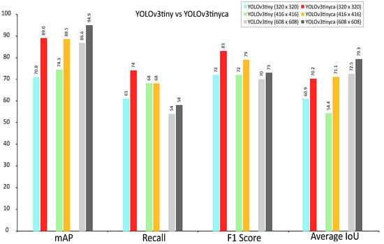
Figure 22.
Comparison of mAP, recall, F1 score, and average IoU of the YOLOv3-tiny and YOLOv3-tinyca models. Dark coloured bars represent the optimised results.
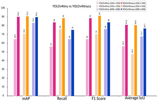
Figure 23.
Comparison of mAP, recall, F1 score, and average IoU of the YOLOv4-tiny and YOLOv4-tinyca models. Dark coloured bars represent the optimised results.
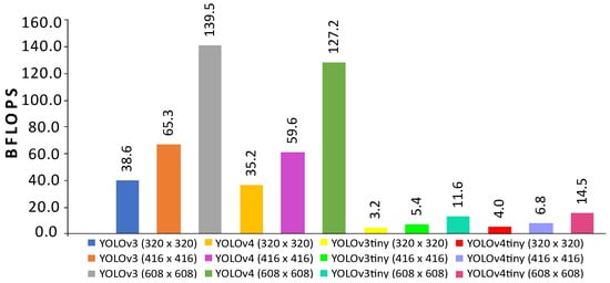
Figure 24.
BFLOPS values for the YOLO v3, v4, and tiny versions.
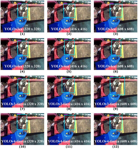
Figure 25.
Qualitative analysis of YOLO with custom anchors (1–12 of Table 8) on a sample image.
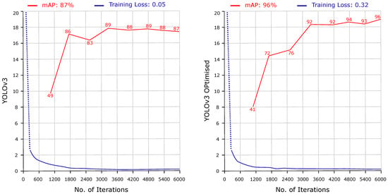
Figure 26.
mAP (red) and training loss (blue) of YOLOv3 and corresponding optimised model.
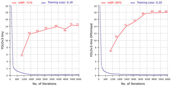
Figure 27.
mAP (red) and training loss (blue) of YOLOv3-tiny and corresponding optimised model.
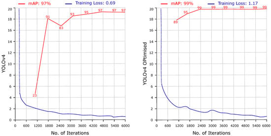
Figure 28.
mAP (red) and training loss (blue) of YOLOv4 and corresponding optimised model.
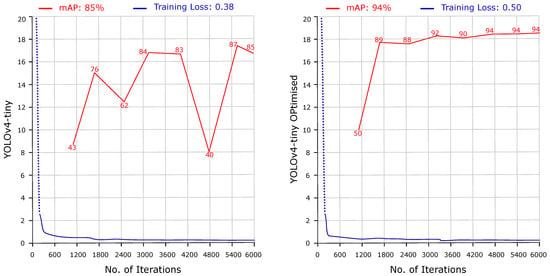
Figure 29.
mAP (red) and training loss (blue) of YOLOv4-tiny and corresponding optimised model.
6. Discussion
We presented our work in Section 3 and compared the performance of single- and multi-stage object detectors for their speed and accuracy. The results are evaluated on a test set of 3020 images and presented in tables, figures, and charts. The first part of the experiments includes Faster R-CNN, SSD, and lightweight MobileNets. The results indicate that Faster R-CNN achieved a higher mAP of 88.8% trained with the three different backbones, i.e., Inception v2, ResNet-50, and ResNet-101. The FPS value declined with the selection of a larger input size. The SSD was three times faster, with a reduction of 13.1% in precision, than Faster R-CNN. We observed increased training and run-time costs for large backbone networks like ResNet-101. The training loss remained lower in most trials. The results show a trade-off between speed and accuracy for the single- and multi-stage object detectors. The combination of SSD and MobileNets achieved balanced speed and accuracy; however, they need further modifications to perform real-time object detection. MobilelNets V3 improved over its predecessor versions in terms of its overall performance. YOLO (v3, v4) is an alternative for object detection, which can produce improved detection results. Identifying crabs and lobsters onboard fishing boats is challenging due to different lighting conditions, camera setups, backgrounds, etc., and thus requires an efficient object detection mechanism. We applied the k-means clustering algorithm to generate custom anchors and trained YOLO on our large dataset. The comparison of the results shows that the performance of the single-stage YOLO object detector is improved. The optimised YOLOv4 and it’s tiny variant achieved mAP of 99.2% and 95.2%, respectively. They are well-suited for detecting crabs and lobsters on fishing boats. We will extend the work on the proposed fisheries data collection pipeline to include automated measurement, counting, and gender classification of the valuable crustaceans.
7. Conclusions
This paper presents a comprehensive practical analysis of the performance of single- and multi-stage object detectors. We presented an optimised method for detecting crabs and lobsters onboard fishing boats. We provided a novel dataset of 15100 images for training and evaluation purposes. The results indicate a trade-off between speed and accuracy among different types of object detectors. Our solution includes YOLO trained on a custom anchor-based dataset, as described in Section 4. The optimised detector achieved 21% higher results for detecting crabs and lobsters on fishing boats equipped with low-powered hardware. The custom anchor-based YOLO object detector trained on a large dataset can provide an improved solution to detect objects in images. Precise detection of crabs and lobsters will proceed toward the steps of measurement and gender classification in our proposed pipeline for fisheries data collection. Future work will explore image-based counting, mass calculation, and disease detection for the species. The multi-disciplinary research areas include plants, livestock, sea-bed imaging analysis, etc.
Author Contributions
Conceptualisation, M.I., M.N., N.H. and B.T.; methodology, M.I.; software, M.I.; validation, M.I. and B.T.; formal analysis, M.I.; investigation, M.I.; resources, M.I., N.H. and B.T.; data curation, M.I., M.N., N.H. and B.T.; writing—original draft preparation, M.I.; writing—review and editing, M.I., N.H., S.G.D.T. and B.T.; visualisation, M.I.; supervision, B.T. and N.H.; project administration, B.T. and N.H.; funding acquisition, B.T., M.N. and N.H. All authors have read and agreed to the published version of the manuscript.
Funding
This work relates to the UK Department for Environment, Food and Rural Affairs (DeFRA) Fisheries Industry Science Partnership (FISP) funded project ECM_63777 Lot 1—Fisheries Data Collection (UK Seafood Fund Science and Innovation Pillar)—Improving UK shellfish catch composition data and the European Marine and Fisheries Fund and Welsh Government project 81917—Innovation in video and electronic fisheries data capture.
Institutional Review Board Statement
The work reported here was given Aberystwyth University Ethics Approval, Ethics ID #13109.
Informed Consent Statement
Not applicable.
Data Availability Statement
The dataset images are available at https://github.com/ifiaber/Crustaceans (accessed on 9 April 2024).
Acknowledgments
We would like to thank Aberystwyth University, Wales, United Kingdom for the award of Computer Science Department Overseas PhD Scholarship (CSDOPS) to Muhammad Iftikhar for a period of three years to conduct this research. The project is led by Seafish [49] and we would like to thank the staff at Seafish, particularly Lewis Tattersall, for their support. We are thankful to the Australian Fisheries Management Authority (AFMA) for using an image of paper [24]. We are thankful to the reviewers for providing valuable feedback, comments, and suggestions for improving this paper.
Conflicts of Interest
Marie Neal was employed by the company Ystumtec Ltd., Pant-Y-Chwarel, Ystumtuen, Aberystwyth SY23 3AF UK. The remaining authors declare that the research was conducted in the absence of any commercial or financial relationships that could be construed as a potential conflict of interest.
Abbreviations
The following abbreviations are used in this manuscript:
| EM | Electronic Monitoring |
| VMS | Vessel Monitoring System |
| GPU | Graphics Processing Unit |
| FPS | Frames Per Second |
| CNN | Convolutional Neural Network |
| mAP | Mean Average Precision |
| IOU | Intersection Over Union |
| SSD | Singe Shot MultiBox Detector |
| YOLO | You Only Look Once |
| RPN | Region Proposal Network |
| GPM | Geometric Pattern Matching |
| COCO | Common Objects in Context |
| FPN | Feature Pyramid Network |
| CUDA | Compute Unified Device Architecture |
| ReLU | Rectified Linear Unit |
| NLP | Natural Language Processing |
References
- FAO/DANIDA. Fishery and Aquaculture Economics and Policy Division. In Guidelines for the Routine Collection of Capture Fishery Data; FAO Fisheries Technical Paper; FAO: Rome, Italy, 1999; pp. 1–113. [Google Scholar]
- Gilman, E.; Legorburu, G.; Fedoruk, A.; Heberer, C.; Zimring, M.; Barkai, A. Increasing the functionalities and accuracy of fisheries electronic monitoring systems. Aquat. Conserv. Mar. Freshw. Ecosyst. 2019, 29, 901–926. [Google Scholar] [CrossRef]
- Stanley, R.D.; Karim, T.; Koolman, J.; McElderry, H. Design and implementation of electronic monitoring in the British Columbia groundfish hook and line fishery: A retrospective view of the ingredients of success. ICES J. Mar. Sci. 2015, 72, 1230–1236. [Google Scholar] [CrossRef]
- Hold, N.; Murray, L.G.; Pantin, J.R.; Haig, J.A.; Hinz, H.; Kaiser, M.J. Video Capture of Crustacean Fisheries Data as an Alternative to On-board Observers. ICES J. Mar. Sci. 2015, 72, 1811–1821. [Google Scholar] [CrossRef]
- Calderwood, J. Smartphone application use in commercial wild capture fisheries. Rev. Fish Biol. Fish. 2022, 32, 1063–1083. [Google Scholar] [CrossRef] [PubMed]
- Barbedo, J.G.A. A Review on the Use of Computer Vision and Artificial Intelligence for Fish Recognition, Monitoring, and Management. Fishes 2022, 7, 335. [Google Scholar] [CrossRef]
- Gladju, J.; Kamalam, B.S.; Kanagaraj, A. Applications of data mining and machine learning framework in aquaculture and fisheries: A review. Smart Agric. Technol. 2022, 2, 100061. [Google Scholar] [CrossRef]
- The United Nations Decade of Ocean Science for Sustainable Development (2021–2030) Implementation Plan. Intergovernmental Oceanographic Commission of the United Nations Educational, Scientific and Cultural Organization: Paris, France, 2021; pp. 1–54.
- Iftikhar, M.; Tiddeman, B.; Neal, M.; Hold, N.; Neal, M. Investigating deep learning methods for identifying crabs and lobsters on fishing boats. In Proceedings of the 41st Computer Graphics and Visual Computing Conference (CGVC), Aberystwyth, UK, 14–15 September 2023. [Google Scholar]
- Toé, S.G.D.; Neal, M.; Hold, N.; Heney, C.; Turner, R.; Mccoy, E.; Iftikhar, M.; Tiddeman, B. Automated video-based capture of crustacean fisheries data using low-power hardware. Sensors 2023, 23, 7897. [Google Scholar] [CrossRef]
- Zou, Z.; Chen, K.; Shi, Z.; Guo, Y.; Ye, J. Object detection in 20 years: A survey. Proc. IEEE 2023, 11, 257–276. [Google Scholar] [CrossRef]
- Redmon, J.; Divvala, S.; Girshick, R.; Farhadi, A. You Only Look Once: Unified, Real-Time Object Detection. In Proceedings of the IEEE Conference on Computer Vision and Pattern Recognition, Las Vegas, NV, USA, 26 June–1 July 2016; pp. 779–788. [Google Scholar]
- Redmon, J.; Farhadi, A. You Only Look Once: YOLO9000: Better, Faster, Stronger. In Proceedings of the IEEE conference on Computer Vision and Pattern Recognition, Honolulu, HI, USA, 21–26 July 2017; pp. 7263–7271. [Google Scholar]
- Redmon, J.; Farhadi, A. Yolov3: An incremental improvement. arXiv 2018, arXiv:1804.02767. [Google Scholar]
- Bochkovskiy, A.; Wang, C.Y.; Liao, H.Y.M. Yolov4: Optimal speed and accuracy of object detection. arXiv 2020, arXiv:2004.10934. [Google Scholar]
- Ren, S.; He, K.; Girshick, R.; Sun, J. Faster r-cnn: Towards real-time object detection with region proposal networks. IEEE Trans. Pattern Anal. Mach. Intell. 2016, 39, 1137–1149. [Google Scholar] [CrossRef] [PubMed]
- Chen, J.; Dai, X.; Chen, D.; Liu, M.; Dong, X.; Yuan, L.; Liu, Z. Mobile-former: Bridging mobilenet and transformer. In Proceedings of the IEEE/CVF Conference on Computer Vision and Pattern Recognition, New Orleans, LA, USA, 19–20 June 2022; pp. 5270–5279. [Google Scholar]
- Nouby, A.E.; Touvron, H.; Caron, M.; Bojanowski, P.; Douze, M.; Joulin, A.; Laptev, I.; Neverova, N.; Synnaeve, G.; Verbeek, J.; et al. Xcit: Cross-covariance image transformers. Adv. Neural Inf. Process. Syst. 2021, 34, 20014–20027. [Google Scholar]
- Liu, Z.; Lin, Y.; Cao, Y.; Hu, H.; Wei, Y.; Zhang, Z.; Lin, S.; Guo, B. Swin transformer: Hierarchical vision transformer using shifted windows. In Proceedings of the IEEE/CVF International Conference on Computer Vision, Montreal, BC, Canada, 11–17 October 2021; pp. 10012–10022. [Google Scholar]
- Wang, W.; Xie, E.; Li, X.; Fan, D.P.; Song, K.; Liang, D.; Lu, T.; Luo, P.; Shao, L. Pyramid vision transformer: A versatile backbone for dense prediction without convolutions. In Proceedings of the IEEE/CVF International Conference on Computer Vision, Montreal, BC, Canada, 11–17 October 2021; pp. 568–578. [Google Scholar]
- Allken, V.; Rosen, S.; Handegard, N.O.; Malde, K. A deep learning-based method to identify and count pelagic and mesopelagic fishes from trawl camera images. ICES J. Mar. Sci. 2021, 78, 3780–3792. [Google Scholar] [CrossRef]
- Allken, V.; Rosen, S.; Handegard, N.O.; Malde, K. A real-world dataset and data simulation algorithm for automated fish species identification. Geosci. Data J. 2021, 8, 199–209. [Google Scholar] [CrossRef]
- Cai, K.; Miao, X.; Wang, W.; Pang, H.; Liu, Y.; Song, J. A modified YOLOv3 model for fish detection based on MobileNetv1 as backbone. Aquac. Eng. 2020, 91, 102117. [Google Scholar] [CrossRef]
- Qiao, M.; Wang, D.; Tuck, G.N.; Little, L.R.; Punt, A.E.; Gerner, M. Deep learning methods applied to electronic monitoring data: Automated catch event detection for longline fishing. ICES J. Mar. Sci. 2021, 78, 25–35. [Google Scholar] [CrossRef]
- Salman, A.; Siddiqui, S.A.; Shafait, F.; Mian, A.; Shortis, M.R.; Khurshid, K.; Ulges, A.; Schwanecke, U. Automatic fish detection in underwater videos by a deep neural network-based hybrid motion learning system. ICES J. Mar. Sci. 2020, 77, 1295–1307. [Google Scholar] [CrossRef]
- Tseng, C.H.; Kuo, Y.F. Detecting and counting harvested fish and identifying fish types in electronic monitoring system videos using deep convolutional neural networks. ICES J. Mar. Sci. 2020, 77, 1367–1378. [Google Scholar] [CrossRef]
- Cao, S.; Zhao, D.; Liu, X.; Sun, Y. Real-time robust detector for underwater live crabs based on deep learning. Comput. Electron. Agric. 2020, 172, 105339. [Google Scholar] [CrossRef]
- Chen, X.; Zhang, Y.; Li, D.; Duan, Q. Chinese Mitten Crab Detection and Gender Classification Method Based on Gmnet-Yolov4. Comput. Electron. Agric. 2023, 214, 108318. [Google Scholar] [CrossRef]
- Ji, W.; Peng, J.; Xu, B.; Zhang, T. Real-time detection of underwater river crab based on multi-scale pyramid fusion image enhancement and MobileCenterNet model. Comput. Electron. Agric. 2023, 204, 107522. [Google Scholar] [CrossRef]
- Wu, C.; Xie, Z.; Chen, K.; Shi, C.; Ye, Y.; Xin, Y.; Zarei, R.; Huang, G. A Part-based Deep Learning Network for identifying individual crabs using abdomen images. Front. Mar. Sci. 2023, 10, 1093542. [Google Scholar] [CrossRef]
- Wang, D.; Vinson, R.; Holmes, M.; Seibel, G.; Tao, Y. Convolutional neural network guided blue crab knuckle detection for autonomous crab meat picking machine. Opt. Eng. 2018, 57, 043103. [Google Scholar] [CrossRef]
- Otsu, N. A threshold selection method from gray-level histograms. IEEE Trans. Syst. Man Cybern. 1979, 9, 62–66. [Google Scholar] [CrossRef]
- Wang, D.; Holmes, M.; Vinson, R.; Seibel, G.; Tao, Y. Machine Vision Guided Robotics for Blue Crab Disassembly—Deep Learning Based Crab Morphology Segmentation. In Proceedings of the ASABE Annual International Meeting, American Society of Agricultural and Biological Engineers, Detroit, MI, USA, 29 July–1 August 2018; p. 1. [Google Scholar]
- Chelouati, N.; Bouslimani, Y.; Ghribi, M. Lobster Position Estimation Using YOLOv7 for Potential Guidance of FANUC Robotic Arm in American Lobster Processing. Designs 2023, 7, 70. [Google Scholar] [CrossRef]
- Cao, S.; Zhao, D.; Sun, Y.; Ruan, C. Learning-based low-illumination image enhancer for underwater live crab detection. ICES J. Mar. Sci. 2021, 78, 979–993. [Google Scholar] [CrossRef]
- Mahmood, A.; Bennamoun, M.; An, S.; Sohel, F.; Boussaid, F.; Hovey, R.; Kendrick, G. Automatic detection of Western rock lobster using synthetic data. ICES J. Mar. Sci. 2020, 77, 1308–1317. [Google Scholar] [CrossRef]
- Chelouati, N.; Fares, F.; Bouslimani, Y.; Ghribi, M. Lobster detection using an Embedded 2D Vision System with a FANUC industrual robot. In Proceedings of the 2021 IEEE International Symposium on Robotic and Sensors Environments (ROSE), Virtual Conference, 28–29 October 2021; pp. 1–6. [Google Scholar]
- Hasan, Y.; Siregar, K. Computer vision identification of species, sex, and age of indonesian marine lobsters. INFOKUM 2021, 9, 478–489. [Google Scholar]
- Li, J.; Xu, W.; Deng, L.; Xiao, Y.; Han, Z.; Zheng, H. Deep learning for visual recognition and detection of aquatic animals: A review. Rev. Aquac. 2023, 15, 409–433. [Google Scholar] [CrossRef]
- Juan, T.; Diana, M.C.E.; Julio, A.R.G. A comprehensive review of yolo architectures in computer vision: From yolov1 to yolov8 and yolo-nas. Mach. Learn. Knowl. Extr. 2023, 5, 1680–1716. [Google Scholar] [CrossRef]
- Jiao, L.; Zhang, F.; Liu, F.; Yang, S.; Li, L.; Feng, Z.; Qu, R. A survey of deep learning-based object detection. IEEE Access 2019, 7, 128837–128868. [Google Scholar] [CrossRef]
- Lin, T.Y.; Dollár, P.; Girshick, R.; He, K.; Hariharan, B.; Belongie, S. Feature pyramid networks for object detection. In Proceedings of the IEEE conference on computer vision and pattern recognition, Honolulu, HI, USA, 21–26 July 2017; pp. 2117–2125. [Google Scholar]
- He, K.; Zhang, X.; Ren, S.; Sun, J. Spatial pyramid pooling in deep convolutional networks for visual recognition. IEEE Trans. Pattern Anal. Mach. Intell. 2015, 37, 1904–1916. [Google Scholar] [CrossRef] [PubMed]
- Liu, S.; Qi, L.; Qin, H.; Shi, J.; Jia, J. Path aggregation network for instance segmentation. In Proceedings of the IEEE Conference on Computer Vision and Pattern Recognition, Salt Lake City, UT, USA, 19–21 June 2018; pp. 8759–8768. [Google Scholar]
- Liu, W.; Anguelov, D.; Erhan, D.; Szegedy, C.; Reed, S.; Fu, C.Y.; Berg, A.C. Ssd: Single shot multibox detector. In Proceedings of the Computer Vision–ECCV 2016: 14th European Conference, Amsterdam, The Netherlands, 11–14 October 2016; pp. 21–37. [Google Scholar]
- Available online: https://pypi.org/project/labelImg/ (accessed on 12 January 2024).
- Na, S.; Xumin, L.; Yong, G. Research on k-means clustering algorithm: An improved k-means clustering algorithm. In Proceedings of the 2010 Third International Symposium on Intelligent Information Technology and Security Informatics, Jian, China, 2–4 April 2010; pp. 63–67. [Google Scholar]
- Available online: https://www.learnbymarketing.com/methods/k-means-clustering/ (accessed on 12 January 2024).
- seafish.co.uk. Available online: https://seafish.org (accessed on 9 April 2024).
Disclaimer/Publisher’s Note: The statements, opinions and data contained in all publications are solely those of the individual author(s) and contributor(s) and not of MDPI and/or the editor(s). MDPI and/or the editor(s) disclaim responsibility for any injury to people or property resulting from any ideas, methods, instructions or products referred to in the content. |
© 2024 by the authors. Licensee MDPI, Basel, Switzerland. This article is an open access article distributed under the terms and conditions of the Creative Commons Attribution (CC BY) license (https://creativecommons.org/licenses/by/4.0/).


