Article

An Improved Ensemble-Based Cardiovascular Disease Detection System with Chi-Square Feature Selection

1
Computer Engineering Department, University of Technology-Iraq, Baghdad 10001, Iraq
2
Control and Systems Engineering Department, University of Technology-Iraq, Baghdad 10001, Iraq
*
Author to whom correspondence should be addressed.
Computers 2024, 13(6), 126; https://doi.org/10.3390/computers13060126
Submission received: 12 April 2024 / Revised: 14 May 2024 / Accepted: 20 May 2024 / Published: 22 May 2024
(This article belongs to the Special Issue Machine and Deep Learning in the Health Domain 2024)

Abstract

:
Cardiovascular disease (CVD) is a leading cause of death globally; therefore, early detection of CVD is crucial. Many intelligent technologies, including deep learning and machine learning (ML), are being integrated into healthcare systems for disease prediction. This paper uses a voting ensemble ML with chi-square feature selection to detect CVD early. Our approach involved applying multiple ML classifiers, including naïve Bayes, random forest, logistic regression (LR), and k-nearest neighbor. These classifiers were evaluated through metrics including accuracy, specificity, sensitivity, F1-score, confusion matrix, and area under the curve (AUC). We created an ensemble model by combining predictions from the different ML classifiers through a voting mechanism, whose performance was then measured against individual classifiers. Furthermore, we applied chi-square feature selection method to the 303 records across 13 clinical features in the Cleveland cardiac disease dataset to identify the 5 most important features. This approach improved the overall accuracy of our ensemble model and reduced the computational load considerably by more than 50%. Demonstrating superior effectiveness, our voting ensemble model achieved a remarkable accuracy of 92.11%, representing an average improvement of 2.95% over the single highest classifier (LR). These results indicate the ensemble method as a viable and practical approach to improve the accuracy of CVD prediction.

1. Introduction

The heart, an essential organ, supplies oxygen and nutrients to the body. “Cardiovascular disease (CVD)” or “heart disease (HD)” refers to a wide range of conditions that affect the heart and blood arteries, including high blood pressure, valvular heart disease, arrhythmia, and coronary artery disease [1,2,3]. According to World Health Organization (WHO) statistics, CVD contributes significantly to global mortality rates [4], emphasizing the importance of early detection in reducing mortality. However, detecting CVD early poses challenges because many heart conditions do not develop symptoms until they are significantly advanced [5]. Traditional diagnostic methods for CVD, such as vital sign analysis, physical examinations, and electrocardiograms, can be time-consuming, error-prone, and require human manual intervention [6]. Therefore, these methods might overlook early signs of CVD, which means patients end up in a worse condition due to treatment delays. As a result, advanced computer-aided techniques for automatic diagnosis using cardiac data have been developed [7].
The fast evolution of artificial intelligence (AI) methods in healthcare has resulted in more precise diagnosis of CVD. The goal of AI research and development is to develop intelligent machines that can carry out human-like tasks. AI-driven diagnosis systems can analyze vast amounts of data more accurately than traditional methods. Also, these systems can automate the diagnosis of routine tasks and detect health risks before they become apparent [8,9].
One of the most popular AI approaches is machine learning (ML), which trains computers to make decisions like those made by humans [10]. Several ML approaches have been studied by researchers to predict HD early on [11]. The most used ML techniques for HD prediction include fuzzy logic, decision trees, logistic regression (LR), k-nearest neighbor (K-NN), naïve bayes (NB), support vector machines (SVM), and others [12]. Currently, researchers are suggesting ML techniques such as ensemble models as more efficient methods for identifying CVD. Ensemble models incorporate predictions from numerous distinct base models (M1, M2, M3, … Mn) to enhance the overall accuracy of predictions [13,14]. There have been attempts to compare ensemble versions of ML models with single-base ML models to find the most accurate diagnosis tool [15]. Ensemble ML models have demonstrated good classification accuracy, proving their value in predicting CVD [16]. However, only a limited amount of research has explored ensemble models for predicting HD [15].
A significant challenge in high-accuracy prediction is managing numerous attributes, which can lead to overfitting—model performance decreases due to learning too much from the training data [17]. Optimal feature selection methods have been identified as an essential strategy to enhance the capabilities of ML algorithms to predict CVD [18] by prioritizing the most relevant features to increase accuracy [19].
Unlike many other research studies that only focus on prediction model accuracy, our study focuses on both computational efficiency and high predictive accuracy. Our work is one of the few that presents an approach to combine feature selection with ensemble learning to enhance CVD diagnosis. To achieve this approach, we utilize a voting ensemble of multiple ML classifiers and the chi-square feature selection method. This combination allows for a significant reduction in feature space without compromising the prediction accuracy. This approach improves the scalability and efficiency of the model, which is important for practical use. As such, the main objective of our study is to build and evaluate an advanced AI-based system for early detection of CVD. The main contributions of this study can be summarized in the following points:
  • To develop a CVD detection system with a voting ensemble model that combines various ML model predictions to reduce the overall error and increase accuracy.
  • To implement a chi-square feature selection algorithm to extract the features that are most useful, aiming to decrease the computation time and enhance prediction accuracy.
  • To evaluate the performance of the proposed CVD detection system by comparing it with existing systems using various performance metrics.
  • The paper is organized as follows: Section 2 reviews previous research on the use of ensemble ML models for HD detection and prediction; Section 3 outlines our methodology, which includes detailed explanations of data collection, pre-processing, the chi-square feature selection algorithm, and the ML models used; Section 4 presents the experimental results and compares them with existing methodologies; Section 5 concludes the paper by summarizing our findings and their implications.

2. Related Work

The usage of machine learning (ML) to enhance cardiovascular disease (CVD) diagnosis has led to significant advances in medicine and healthcare. Ensemble learning techniques have become more widespread recently to develop more accurate predictive models for diagnosing CVD based on clinical data. However, many features may affect the final diagnosis when analyzing medical data. Therefore, to improve the accuracy of predictive models, many researchers are employing feature selection techniques that identify the most important features [20]. Many studies have proposed enhanced ensemble learning techniques with optimum feature selection methods for the detection of cardiac diseases.
Study [21] used ML classifiers combined with deep-learning (DL) classifiers in a voting ensemble model to accurately predict heart diseases. Researchers made use of six different classifiers—RF, KNN, DT, XGB, DNN, and KDNN—to achieve an accuracy of 88.70%. Both [11] and [19] proposed a voting ensemble classifier that combines predictions from multiple individual classifiers to improve heart disease prediction accuracy. After processing the Cleveland dataset, both studies used extra tree feature selection to identify key features. Researchers in [11] combined NB, artificial neural network (ANN), logistic regression (LR), decision tree (DT), and k-nearest neighbor (KNN) using ensemble voting and majority bagging methods. Meanwhile in [19], only SVM, NB, and LR were combined. Both studies showed the superiority of bagging and voting ensemble methods over the individual classifiers, with 87.78% and 84.79% accuracy, respectively.
Also, Ref. [18] proposed an ensemble ML approach combined with chi-square and recursive feature elimination (RFE) to diagnose heart diseases. Among the several ML models employed, classification and regression trees (CART) produced the highest accuracy (87.65%). In addition, Ref. [22] examined ensemble approaches that combine different base classifiers—NB, RF, C4.5, Bayesian network, multilayer perceptron (MLP), and projective adaptive resonance theory (PART)—to improve the accuracy of heart disease prediction. The ensemble approaches—bagging, boosting, majority voting, and stacking—were developed and optimized using a feature selection method. By employing a 10-fold cross-validation method with the Cleveland dataset, the basic classifiers and ensemble techniques were evaluated. The results revealed that the ensemble approach (majority voting) improved the accuracy by 7.26% for weak classifiers, such as C4.5, MLP, and PART.
Similarly, Ref. [23] created an ensemble model optimized with correlation feature selection (CFS) and particle swarm optimization (PSO) to identify cardiac disease with an 85.71% accuracy rate. The ensemble model utilized gradient boosting (GB), extreme gradient boosting (XGB), and random forest classifiers. Furthermore, Ref. [24] proposed a voting ensemble model using base ML models of SVM, DT, and ANN to predict heart disease. Both the base and voting ensemble models were trained using the partitioned, pre-processed Cleveland dataset. After evaluating all models in terms of accuracy, precision, recall, and F1-score, the voting ensemble model outperformed the base models in terms of accuracy (87.3%), precision (82.8%), recall (90.8%), and F1-score (87.1%).
Additionally, a novel voting strategy based on ensemble learning was proposed in [25], which made use of six ML algorithms: NB, SVM, DT, neural network (NN), MLP, and single-layer perceptron. The researchers found that, on average, the ensemble model achieved 83% accuracy, which was higher than any of the individual methods. Also, Ref. [26] combined deep-learning strategies (long short-term memory (LSTM) and gated recurrent unit (GRU) neural networks) with machine-learning techniques (RF, SVM, and KNN) to develop a voting ensemble model. Individual models trained and tested on the Cleveland dataset achieved prediction accuracy between 75% and 86%. In contrast, the voting ensemble model outperformed the individual models by 2.1%. Similarly, Ref. [27] proposed an ensemble framework for predicting heart disease. The ensemble model obtained an accuracy of 87.05% for majority voting of SVM, NB, and ANN algorithms.

3. Materials and Methods

The following sections explain the two main steps to achieve this study’s objectives. Section 3.1 details the working process related to the proposed ensemble machine-learning model for heart disease identification. This section comprehensively explains the stages of ensemble model development, from data collection and feature scaling to selecting and evaluating appropriate machine-learning models. Section 3.2 presents details regarding the feature selection method, which aims to improve the performance of the proposed ensemble model for cardiac disease prediction.

3.1. Ensemble Model

Figure 1 provides a detailed overview of how the proposed system operates. The proposed ensemble machine-learning (ML)-based prediction system includes four significant stages: data pre-processing, feature selection using the chi-square method, training ML models, and creating a majority voting ensemble model. As part of the pre-processing phase, we used the standard feature scaling method. During the feature selection stage, the most important features were chosen using the chi-square statistical algorithm.
We used the UCI Cleveland dataset [28], since it contains clinically important features needed to diagnose cardiac disease. The four individual ML models (logistic regression (LR), random forest (RF), naïve Bayes (NB), k-nearest neighbor (KNN)) were trained with fewer features. NB and LR handle linear separations well; RF handles complex structures without overfitting; and KNN is simple and effective at capturing complex patterns without assuming a data distribution. This diversity in modeling approaches uses the strengths of various methods to increase the predicted accuracy.
Using the testing data, each trained standalone ML model performed its own classification, and an ensemble model was created by combining the predictions from these models using a voting classifier. In ensemble learning, the predictions from different separate classifiers (M1, M2, M3, … Mn) combine to achieve a stronger classifier with better predictive performance [13]. Using the scikit-learn and Python libraries, we were able to create and test the suggested system for the prediction of cardiac disease [29].

3.1.1. Heart Disease (HD) Dataset and Pre-Processing

For this study, a public dataset, the Cleveland heart disease dataset, was obtained from the University of California at Irvine (UCI) machine-learning repository. This dataset is largely employed by many researchers to predict the occurrence of cardiac conditions [30]. Although the Cleveland dataset has 303 records and 76 attributes, many researchers often employ 14 of them in their experimentation. There are thirteen (13) input features: age, gender, cholesterol, heart rate, chest pain type, fasting blood sugar, blood pressure, resting ECG, exercise-induced angina, ST slope, ST depression, number of significant vessels colored by fluoroscopy, and thalassemia. The last output feature indicates whether the person has cardiac disease or not by using binary values of 0 and 1 [31]. Table 1 shows comprehensive details regarding the dataset’s attributes. There were no missing values in the obtained dataset. However, the data distribution was uneven for some features, including cholesterol, heart rate, blood pressure, and age; this could cause inaccurate predictions when training the model. Consequently, to obtain a normal distribution of the data, the standard feature scaling method was used in the pre-processing phase. To find the new standardized data point ( x s t d ), this method first subtracts the mean ( μ ) from each data point ( x i ) and then divides the result by the standard deviation ( σ ), as shown in Equation (1) [32].
x s t d = x i μ σ

3.1.2. Machine-Learning (ML) Models

ML employs many methods and strategies for the diagnosis of heart disorders. The main ML models used in this study’s methodology are detailed in the sections that follow:
(a)
Logistic Regression (LR)
LR is a common ML model often used for regression tasks. However, this model is also widely used for binary classification tasks, where the probability of a categorical target variable is predicted [33]. Although it is particularly efficient for binary classification problems, it may also be used for multiclass classification utilizing multinomial logistic regression [34]. The LR model assumes that the data follow a Bernoulli distribution and fits the parameters using the maximum likelihood function with gradient descent for classifying the data [35]. It utilizes a non-linear function, such as sigmoid or logistic function, for identifying the class of new input [19,36]. The following is an expression that depicts the generic form of the logistic regression model [37]:
P Y = 1 = 1 1 + e ( β 0 + β 1 X 1 + β 2 X 2 + + β n X n )
where  Y  denotes the binary outcome variable;  β 0  denotes the intercept coefficient; and  β 1 , β 2 , , β n  are the coefficients associated with the features  X 1 , X 2 , , X n , respectively [37].
(b)
Random Forest (RF)
RF is an ensemble ML technique that builds numerous decision trees, each on a randomly selected part of the training data, and then aggregates their predictions [38,39]. RF is effective in both regression and classification tasks. The regression averages the outputs from different trees to make prediction at new point x, as shown in Equation (3) [40].
f ^ r f M ( x ) = 1 M j = 1 M f j ( x )
where  M  represents the number of trees, and  f j  represents  j th decision tree. For classification, it uses majority voting to find out which class received the greatest number of votes among all the trees in the forest. Let  C ^ j x  be the class prediction of  j th decision tree. Then, the prediction at new point  x  is as shown in Equation (4) [41].
C ^ r f M x = m a j o r i t y   v o t e   C ^ j x 1 M
The process of creating less correlated decision trees involves both bagging (bootstrap aggregating) and random feature selection. Through bootstrapping, distinct subsets of the training data are created by random sampling with replacement from the original dataset. This helps in reducing overfitting by providing a more robust and generalizable model [42,43]. At each node of the decision tree, a random subset of features is considered for each split instead of using all features for each split. This helps in decorrelating the trees and introduces diversity in the ensemble. The RF algorithm involves the tuning of multiple hyperparameters, including the n estimators (count of decision trees for growth in the forest), max depth of each decision tree in the forest, criterion (a function used to evaluate split quality at each node of the trees, for example, Gini impurity and information entropy) [42]. More trees in the forest generally results in more reliable and accurate predictions [43].
(c)
Naïve Bayes (NB)
NB is a probabilistic classifier that uses the Bayes theorem with the assumption of conditional independence between features [44]. Conditional independence means that the changes in one feature value are not dependent on the other feature values in a class [39]. This allows the naïve Bayes algorithm to calculate feature distributions  P C X  independently [27]. By decoupling the feature distributions, the naïve Bayes classifier avoids problems caused by high dimensionality, which makes it useful for classifying high dimensional datasets [39]. The naïve Bayes algorithm is built upon the three main basic components of feasibility, antecedent, and prediction. The term “antecedent” refers to information regarding an incident that occurred in the past. The term “feasibility” indicates the possibility that the event will occur in the future. Prediction is based on the first two concepts. Here is the connection between the three of them:
P r e d i c t i o n = A n t e c e d e n t × f e a s i b i l i t y c o r r o b o r a t i o n
The mathematical expression of the relationship mentioned above is
P B A = p a s t   p r o b a b i l i t y × P ( A B ) P ( A )
In Equation (6), there are two possible events: A and B [27]. The NB classifier calculates the posterior probability  P C i X  of each class  C i  based on the input features and predicts the class with the highest probability [40] using the formula given below:
P C i X = P C i × k = 1 n P ( x k | C i ) P ( X )
where  X  is a tuple in the dataset representing  n  features (F1, F2, …, Fn), and  x k  is the value of feature Fk for tuple  X X  will be assigned to the class with the highest posterior probability by the classifier. The naïve Bayes classifier will predict tuples  X  from class  C i  only if
P C i X > P C j X   f o r   1 j m ,   j i
The result is the maximization of  P C i X . The class  C i  where  P C i X  is maximized is referred to as the maximum posteriori hypothesis [22,25]. When compared to other classifiers, the naïve Bayes can be fast, effective, highly scalable, needing just a few parameters, and has the minimum error rate for classification [22,39,44].
(d)
K-Nearest Neighbor (KNN)
KNN is a powerful ML method for regression or classification tasks [21,45]. It is used in cases where the data and labels are known in the given training set [35]. KNN classifies new input data based on their distance from data already classified by K-nearest neighbor [19]. The value of k in a KNN indicates how many nearest neighbors were utilized to create predictions for the input test sample [40]. The selection of the k-nearest neighbors is conducted based on having the smallest distances to the input test sample. Then, the input test sample is placed in the class with the highest frequency of occurrence among the k-nearest neighbor samples [35,45].
Consider the test sample  x t . It finds the training sample ( x 1 y 1 ), which is closest to  x t . Now, predict  y t  as the output  y 1 . In general, instead of considering a single training sample, we consider  i  training samples. To find the distances between a test sample  T ( x 1 T x 2 T ) and each of these  i  training samples  Q i  ( x 1 Q i x 2 Q i ), we compute the Euclidean distance (di) for each pair of points, as shown in Equation (9) [12].
d i = ( x 1 T x 1 Q i ) 2 + ( x 2 T x 2 Q i ) 2
where  Q i  is the  i th training sample. The main parameters of KNN that are configurable include  k  (the number of nearest neighbors), distance function, distance weighting (weighting closer neighbors higher). One common method of weighing is to assign a weight of  1 / d  to each neighbor, where  d  is the distance between neighbors. Tuning these parameters, especially  k , can improve model accuracy [45].
(e)
Voting Classifier (VC)
The majority voting classifier is an ensemble learning technique that aggregates the output of multiple base classifiers provided to it and makes a final prediction of the class label of a new instance based on the majority vote of the individual classifiers [46]. The base classifiers can be of different types (e.g., SVM, logistic regression, naïve Bayes, etc.), which allows ensemble diversity. Each base classifier is trained independently on the same training data and makes predictions on the same testing data. The majority voting classifier then combines these predictions. Each classifier votes for a class label, and the final predicted class label is the one that most base classifiers predicted. The final class label  d j  predicted by the voting classifier is defined as [22]
d j = m o d e l   { C 1 ,   C 2 ,   ,   C m }
where  C 1 , C 2 , , C n  represent the base classifiers, and  m  denotes the quantity of models that are the components of the ensemble. Among the predictions of each base model  C 1 , C 2 , , C m , the model function selects the most common model value [40]. Such a classifier demonstrates its versatility by not only combining different models but also allowing for both hard and soft voting mechanisms. In hard voting, each base classifier votes for a single class label, and the class with most votes is selected as the final output prediction [43]. This is a simple majority voting method.
When using three separate models, the final prediction will reflect the majority opinion. In this case, if two models indicate that class A is the most likely outcome, and the third model indicates that class B is more likely, then class A will be used [40]. In contrast, soft voting takes a more probabilistic approach, averaging the probability estimations provided by each base classifier for each class label and selecting the one with the biggest average probability as the final output prediction [43].

3.2. Enhanced Ensemble Model with Feature Selection (FS)

Issues of underfitting and overfitting training data are common in prediction systems. Underfitting is the process by which a predictive model becomes inaccurate in its predictions because it learns too little from the training data. Overfitting occurs when a prediction model becomes overly dependent on its training data and fails to generalize well to new data [17,47]. The problem of overfitting to training data and improper generalization occurs when a dataset contains an excessive number of irrelevant features. Therefore, to improve the prediction model performance, it is important to choose relevant features and remove irrelevant or noisy features [48,49].
Here, we employed an FS technique based on a chi-square statistical algorithm [50] to choose the features that are most important and eliminate bias from the training set. The chi-square algorithm statistically finds the importance of categorical features related to categorical outcome. It evaluates the independence of each feature with the target variable and provides a score indicating their strength of association. The chi-square algorithm determines the degree of correlation that exists between the input features and the class that is predicted. The chi-square statistic is used for every non-negative feature ( x i ) to find which features are dependent on the predicted class. An increasing chi-square score indicates that the feature is highly dependent on the predicted class [30]. A binary classification problem’s features are ranked using the chi-square test, as follows: assuming there is a total of (t) instances and a positive and negative set of class outputs, Table 2 can be constructed to find the chi-square test score [47].
Where (p) stands for the sum of positive instances; the sum of all non-positive instances is represented by (t − p); (m) stands for the sum of instances in which ( x i ) is present; and (t − m) represents the sum of instances in which ( x i ) is absent.
The chi-square test compares the observed or actual count ( O ) with the expected or predicted count ( E ). The predicted and actual counts are very close when two features are independent. Let  E a E b E c , and  E d  stand for the values that were predicted, and let  a b c , and  d  stand for the values that were measured. Then, Equation (11) can be used, assuming the two events are unrelated, to determine the expected value ( E a ). Likewise,  E b E c , and  E d  are computed. Lastly, the chi-square score is calculated using Equation (13) on which the general chi-square test form given in Equation (12) is based [47].
E a = a + b   ×   a + b t
χ 2 = i = 1 n O i E i 2 E i
χ 2 = a E a 2 E a + b E b 2 E b + c E c 2 E c + d E d 2 E d

4. Result and Discussion

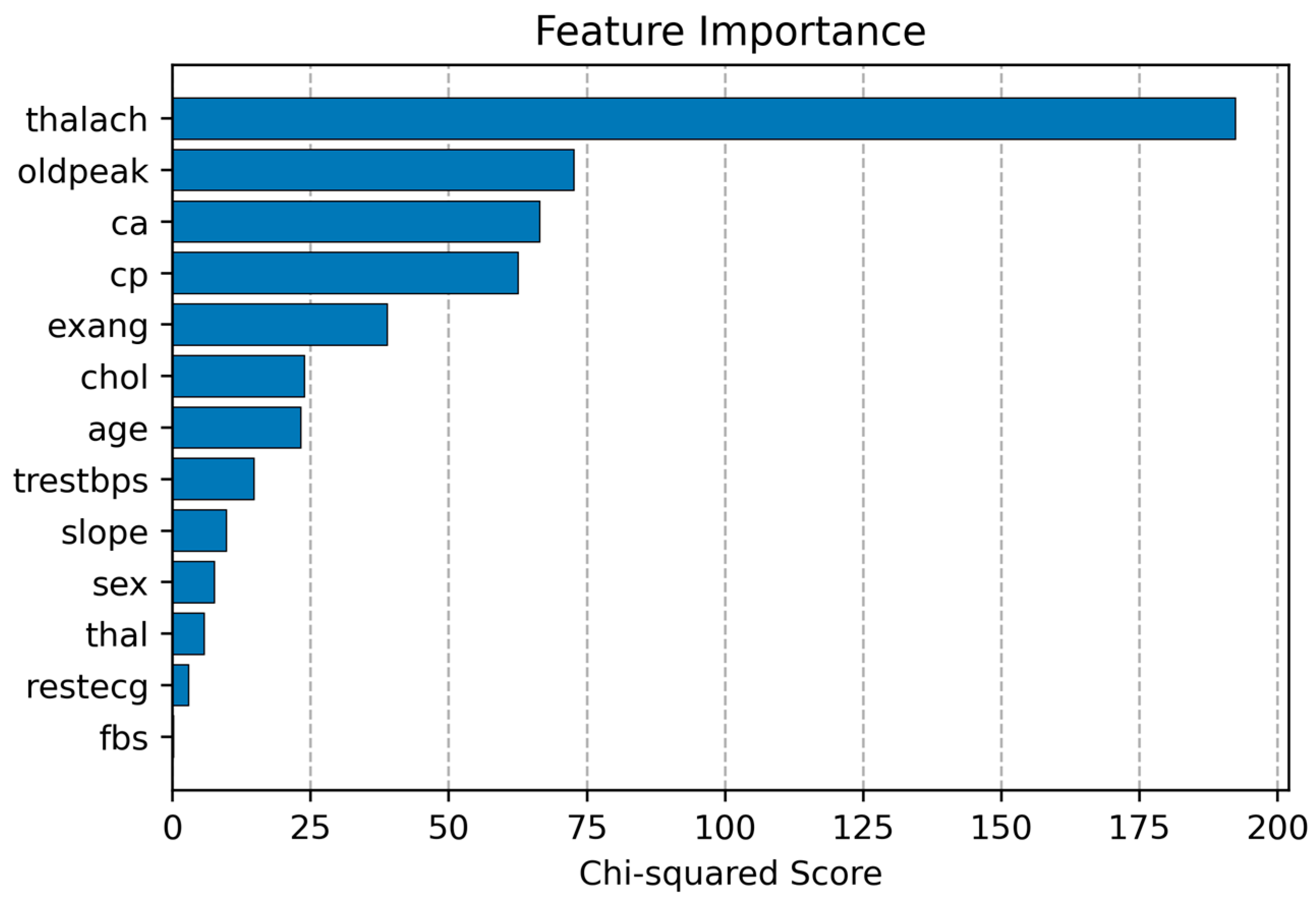
For this study, we implemented the suggested system shown in Figure 1 to diagnose heart disease (HD) using the chi-square feature selection algorithm and a voting ensemble model that included four individual ML models: KNN, NB, RF, LR. The chi-square feature selection (FS) algorithm was utilized on the Cleveland dataset to rank the 13 features according to their importance from highest to lowest, as shown in Figure 2. It recognized the following five most important features for HD diagnosis: thalach, oldpeak, ca, cp, exang. By employing the chi-square method, we reduced the number of features utilized for diagnosis from thirteen to five, thereby reducing the computation load in half.
Next, the collected Cleveland dataset was partitioned into training and testing sets. Whereas the training set is utilized for the aim of training the models, the testing set is employed for producing the prediction outputs from the models and evaluating their performance [51]. In a 75:25 split, the dataset was divided into two parts: one for training and one for testing. This was performed so that a greater portion of the data could be utilized for training purposes.
A prediction model is evaluated based on four main parameters: true negative ( T Negative ) indicates that the algorithm’s predictions for people without HD are accurate; true positive ( T Positive ) indicates that the predictions for patients with HD are accurate; false positive (   F Positive ) indicates that patients without HD are mistakenly classified as having HD; and false negative ( F Negative ) indicates that patients with HD are mistakenly classified as healthy [30]. For the evaluation of the performance of the system that was implemented in this work, the following metrics [52] were used:
  • Accuracy, denoted as Acc, is the proportion of positive model instances to total model instances, as stated in Equation (14).
    Acc = T Positive + T Negative T Positive + T Negative +   F Positive + F Negative
  • Specificity, denoted as Spe, is the proportion of true negatives among all healthy persons, as stated in Equation (15). It is usually used to properly classify persons who are disease-free.
    Spe = T Negative T Negative + F Positive
  • Sensitivity, denoted as Sen, is the proportion of true positives among all unhealthy persons, as stated in Equation (16). It is usually used to properly classify heart disease persons.
    Sen = T Positive T Positive + F Negative
  • F1-score is known as the harmonic mean of sensitivity and specificity, according to Equation (17).
    F 1 - Score = 2 ( T Positive ) 2 ( T Positive ) +   F Positive + F Negative
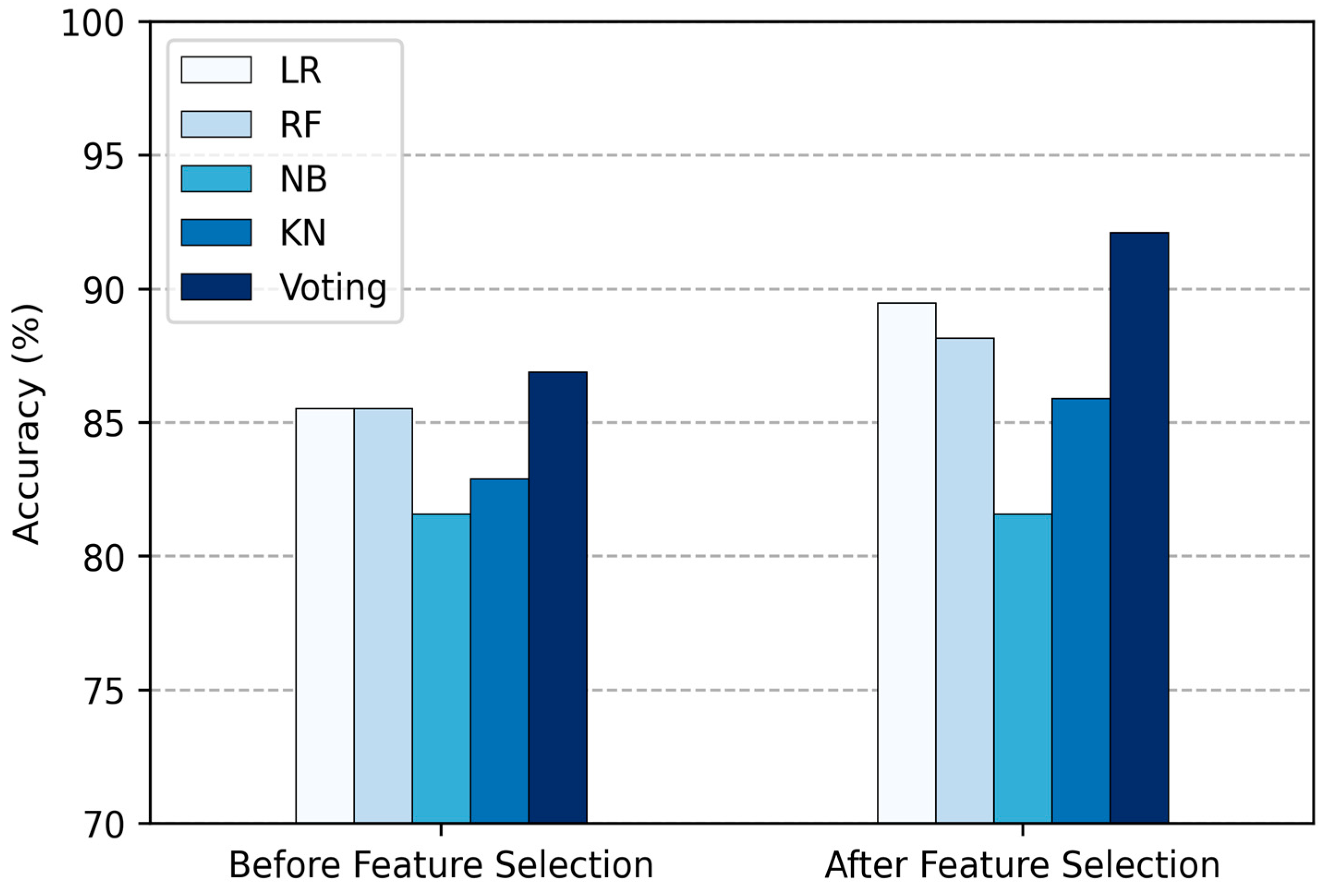
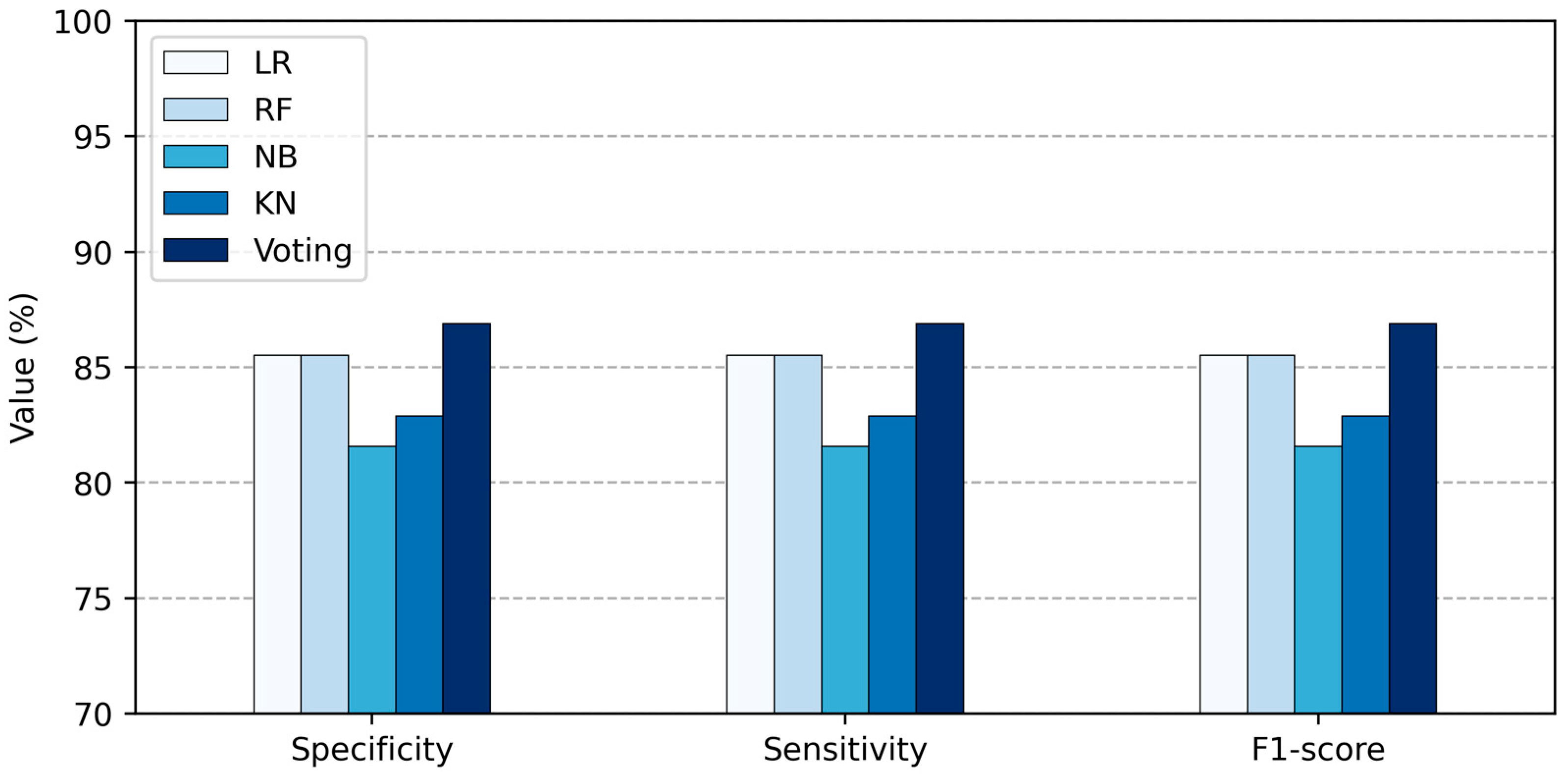
In the evaluation, two approaches were explored. The first approach involved standardizing the Cleveland dataset, which had 13 input features, then directly training and evaluating the individual models (LR, RF, NB, and KNN) without using the chi-square FS algorithm. The base models’ prediction outputs were then aggregated into the voting ensemble classifier. After the base models have produced their predictions, the ensemble classifier checks them for errors and then makes its own prediction. Because of this, the HD diagnosis system was able to improve its overall accuracy while simultaneously decreasing the amount of error produced by each individual base classifier. As shown in Table 3, by using the first approach, the LR and RF classifiers performed well among the other two base classifiers, with the highest accuracy of 85.53% and 85.52%, respectively. KNN and NB had the lowest performance compared to the other base classifiers, with accuracy of 82.89% and 81.58%, respectively. However, the voting ensemble classifier outperformed the base classifiers with an accuracy of 86.84%, showcasing a notable 1.53% enhancement in accuracy for the best performing base classifier (LR).
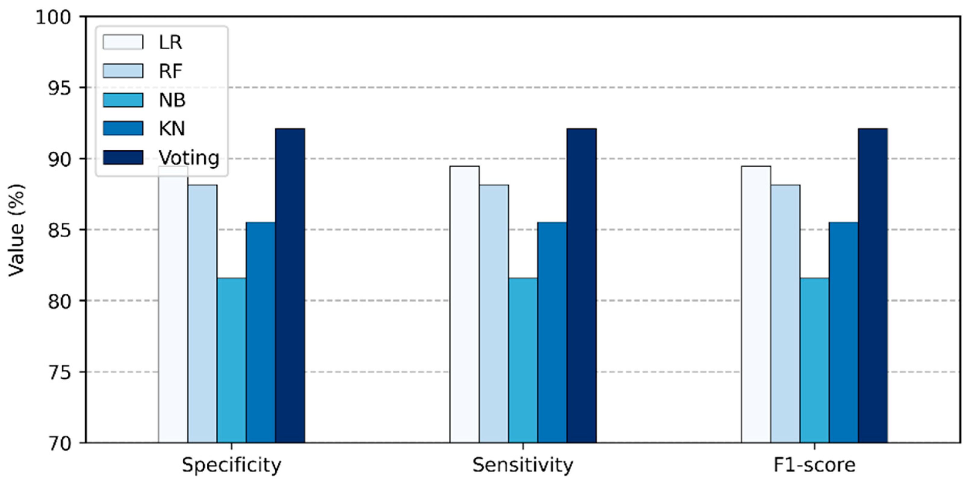
In the second approach, after normalizing the Cleveland dataset using the feature scaling method, the five key features were selected using the chi-square FS algorithm. Afterward, the individual models (LR, RF, NB, and KNN) were trained and evaluated using the reduced-feature dataset. The basis models’ prediction outputs were then fed into the voting ensemble classifier, which produced the final prediction. The accuracy of each base classifier and the ensemble voting classifier after reducing the features is given in Table 4. The results showed a rise in performance for the LR, RF, and KNN models with FS, whereas the NB model showed no improvement at all. The LR, RF, and KNN models achieved accuracy scores of 89.473%, 88.157%, and 85.53%, respectively. Compared to the base models, the voting ensemble classifier performed better, with accuracy of 92.11%, showcasing a notable 2.95% increase over the best performing base classifier (LR). This reveals that using the chi-square FS algorithm with the proposed voting ensemble classifier leads to improved HD diagnosis abilities.
Figure 3 shows the results of a comparison of the two approaches’ prediction accuracy. In the figure, it can be observed that the LR and RF models exhibit comparable performance and have the highest accuracy among the four base classifiers, while the NB and KNN models have lower accuracy in both approaches. It is also evident that voting classifier outperforms the individual algorithms, suggesting that ensemble methods can leverage the strengths of various models to improve overall performance. Also, this figure indicates that the FS method significantly improves the accuracy of the base classifiers and thereby the accuracy of the voting ensemble model by obtaining the highest accuracy rate of 92.11. This marks a 6.07% increase compared to the voting ensemble model without the FS approach. Furthermore, the sensitivity, specificity, and F1-score of the four standalone classifiers as well as the voting ensemble classifier were computed before and after the FS process, as can be seen in Figure 4 and Figure 5. The figures reveal that the suggested vote ensemble classifier outperforms individual classifiers for all the other measurements taking place both before and after the FS process.
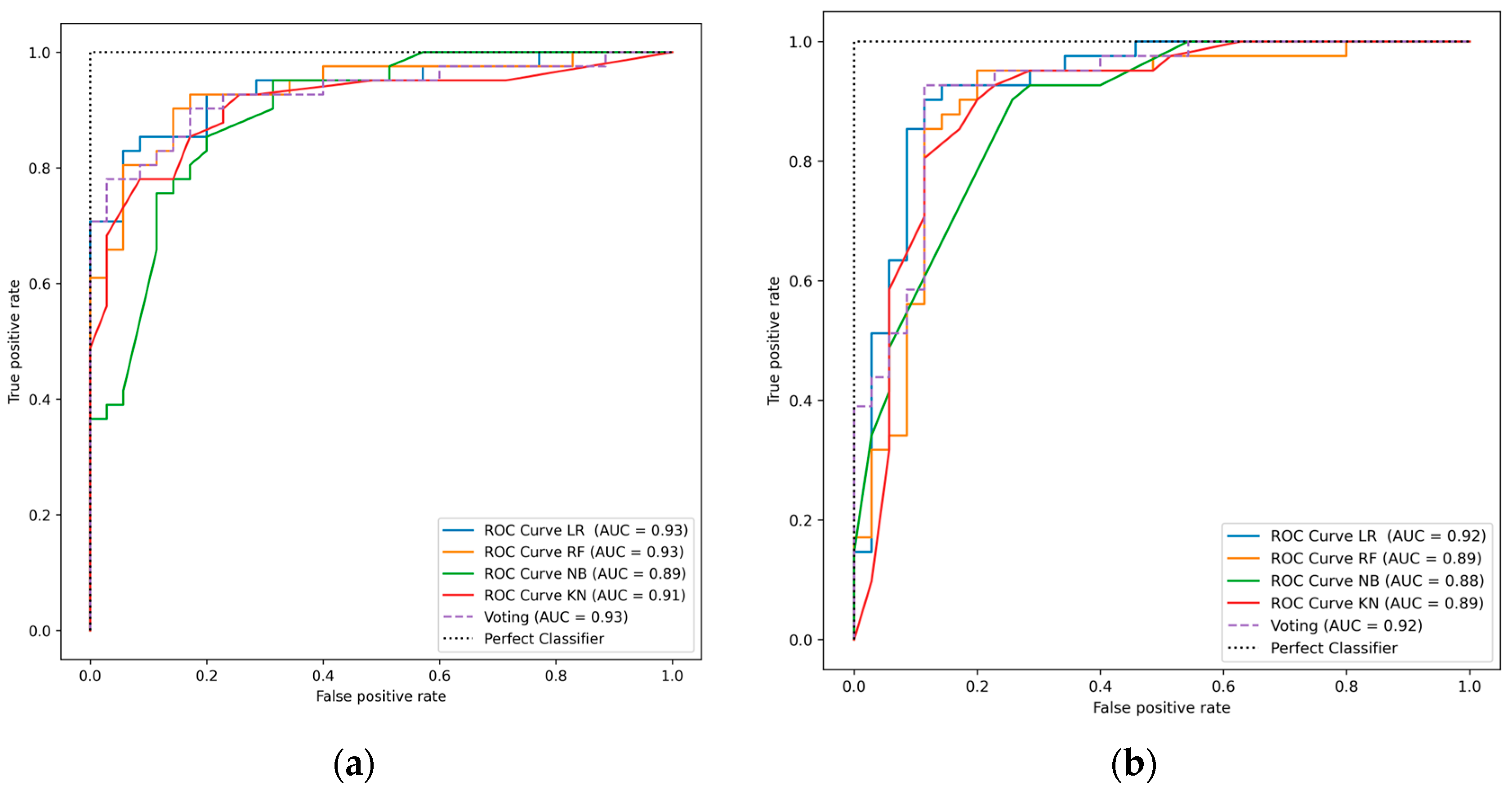
Also, to conduct a more comprehensive evaluation of the diagnostic model’s efficacy, receiver operating characteristic (ROC) and area under the curve (AUC) charts were used. The ROC–AUC plot shows, on the x-axis, the false positive rate and, on the y-axis, the true positive rate. It checks the model’s ability to differentiate between two classes, where 0 indicates no HD and 1 indicates HD. The optimal ROC curve can be found in the top left corner of the plot [47]. When the ROC curve is higher, the model is making accurate predictions between 0 s and 1 s. With an AUC close to 1, the model has strong separability; with an AUC close to 0, it has the worst disassociation. The model lacks the ability to distinguish across classes when the AUC value is 0.5 [53]. Using the ROC–AUC curve, we further evaluated the capability of base classifiers and the voting ensemble classifier in predicting HD, as shown in Figure 6. In the figure, we notice that the AUC score drops after FS for all classifiers. This suggests that the FS approach has little effect on the AUC.
To further evaluate the prediction model’s performance, another parameter called the confusion matrix is employed. The confusion matrix provides a summary of the ratio of incorrect and correct predictions. The rates of true positives ( T Positive ) and false negatives ( F Negative ) are displayed in a table-like format [54].
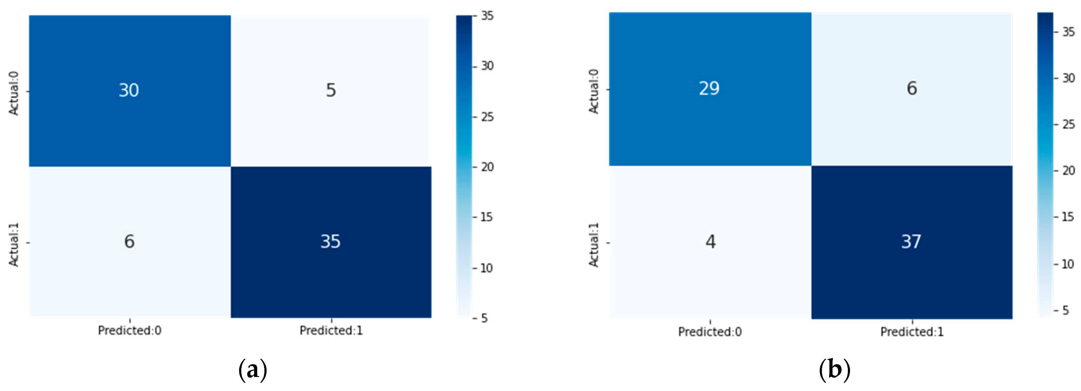
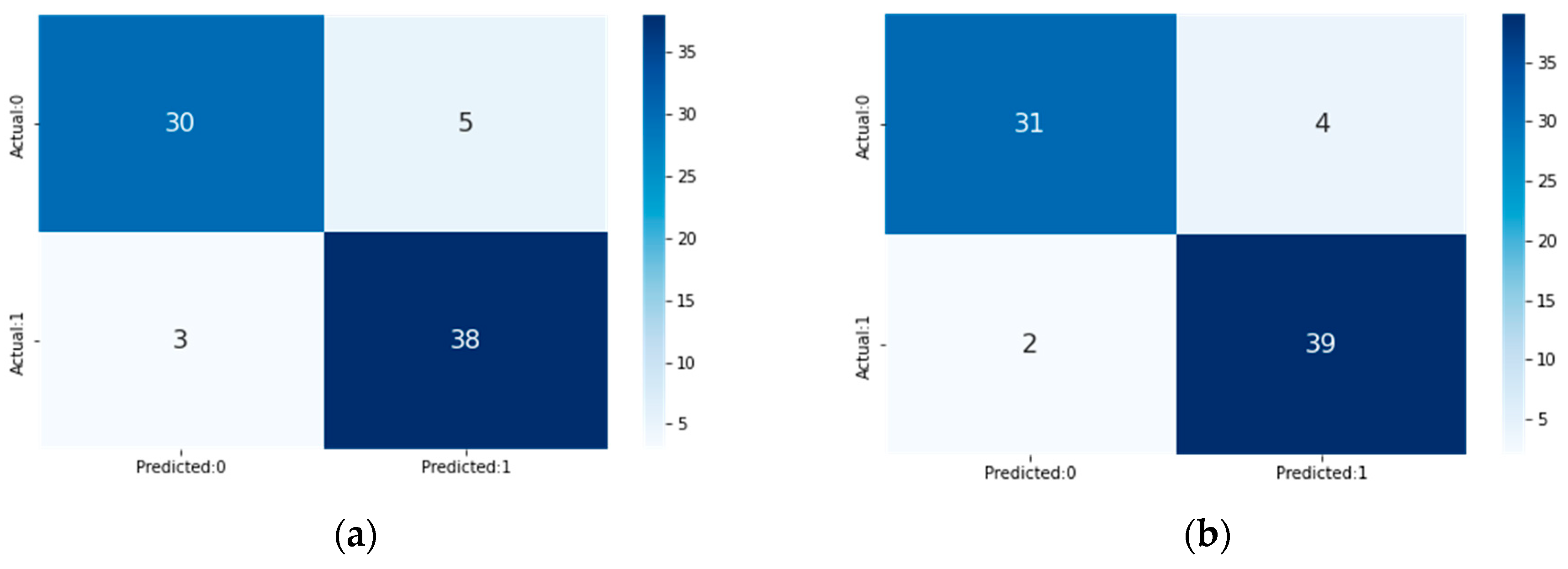
To further assess the efficacy of our voting ensemble classifier and base classifiers in HD diagnosis, we utilized the confusion matrix. The confusion matrices of the best performing base model (LR) and voting ensemble model are shown in Figure 7 and Figure 8, respectively. With the Cleveland dataset, Figure 7 compares the confusion matrices of the voting ensemble model and the best performing base model (LR) that did not use the chi-square FS algorithm. It demonstrates that the LR model can classify 30 out of 35 people as healthy and 35 out of 41 people as unhealthy. Meanwhile, the voting ensemble model can classify 29 out of 35 people as healthy and 37 out of 41 people as unhealthy. This implies that the ensemble voting classifier is better. Figure 8 depicts the confusion matrix of the top-performing base classifier (LR) and the voting ensemble classifier after using the chi-square FS method. The figure shows that out of 35 healthy individuals and 41 HD patients, the LR model accurately identifies 30 and 38, respectively. Meanwhile, the voting ensemble model can correctly identify 31 out of 35 healthy patients and 39 out of 41 patients with HD. This implies that the ensemble voting classifier is better.
Both Figure 7 and Figure 8 demonstrate a decrease from 11 (inaccurate predictions made by the LR) to 8 (inaccurate predictions made by the voting ensemble) and from 10 (inaccurate predictions made by the LR) to 6 (inaccurate predictions made by the voting ensemble) after applying the chi-square FS algorithm.
Finally, as shown in Table 5, we evaluated our ensemble voting model and chi-square-FS-method-based enhanced CVD detection system against multiple state-of-the-art current methods. Here, we looked into how well the classifier performed, the FS method used, and how many features were selected. The suggested chi-square-based voting ensemble model demonstrated an accuracy of 92.11%, which was better than alternative methods. This shows an improvement of 3.84% over the best classifier used in prior research. Our classifier and wearable equipment that tracks the heart rate, blood pressure, and other vital signs can help cardiologists anticipate heart problems in real time before emergency medical aid.

5. Conclusions

This paper introduces an intelligent detection system for CVD diagnosis based on the voting ensemble technique and chi-square feature selection method. The voting ensemble model leveraged diverse base ML models, including logistic regression (LR), random forest (RF), naïve Bayes (NB), and k-nearest neighbor (KNN). The Cleveland heart disease dataset was utilized for the purpose of training and testing both our ensemble and base models. The performance of the models was tested using several different measures, including accuracy, specificity, sensitivity, confusion matrix, F1-score, and area under the curve (AUC). The base classifiers LR, RF, NB, and KNN demonstrated an accuracy of 85.53%, 85.52%, 81.58%, and 82.89%, respectively. Conversely, the voting ensemble classifier surpassed the base classifiers with a superior accuracy of 86.84%. Applying the chi-square feature selection method identified five pertinent features, further enhancing the performance, thereby boosting the accuracy of the voting ensemble model to an impressive 92.11%. The experiments’ results showed that the augmented voting ensemble model that we suggested performed significantly better than the most advanced CVD detection approaches in the current state of the art. In the future, to further demonstrate the significance and generalizability of our methodology, we intend to explore using it with more UCI benchmark datasets.

Author Contributions

Conceptualization, A.E.K. and A.J.H.; methodology, A.E.K.; software, A.E.K.; validation, A.E.K.; formal analysis, A.J.H.; investigation, I.I.G.; resources, A.E.K.; data curation, A.E.K.; writing—original draft preparation, A.E.K.; writing—review and editing, I.I.G.; visualization, A.E.K.; supervision, A.J.H. and I.I.G. All authors have read and agreed to the published version of the manuscript.

Funding

This research received no external funding.

Institutional Review Board Statement

Not applicable.

Informed Consent Statement

Not applicable.

Data Availability Statement

The dataset utilized in this work may be accessed through the machine-learning repository at UCI.

Conflicts of Interest

The authors declare no conflicts of interest.

References

  1. Rajalakshmi, S.; Madhav, K.V. A collaborative prediction of presence of Arrhythmia in human heart with electrocardiogram data using machine learning algorithms with analytics. J. Comput. Syst. Sci. 2019, 15, 278–287. [Google Scholar] [CrossRef]
  2. Hiriyannaiah, S.; Siddesh, G.M.; Kiran, M.H.M.; Srinivasa, K.G. A comparative study and analysis of LSTM deep neural networks for heartbeats classification. Health Technol. 2021, 11, 663–671. [Google Scholar] [CrossRef]
  3. Sakila, V.S.; Dhiman, A.; Mohapatra, K.; Jagdishkumar, P.R. An automatic system for heart disease prediction using perceptron model and gradient descent algorithm. Int. J. Eng. Adv. Technol. 2019, 9, 1506–1509. [Google Scholar] [CrossRef]
  4. World Health Statistics. Available online: https://www.who.int/data/gho/publications/world-health-statistics (accessed on 1 March 2024).
  5. Tan, J.H.; Hagiwara, Y.; Pang, W.; Lim, I.; Oh, S.L.; Adam, M.; Tan, R.S.; Chen, M.; Acharya, U.R. Application of stacked convolutional and long short-term memory network for accurate identification of CAD ECG signals. Comput. Biol. Med. 2018, 94, 19–26. [Google Scholar] [CrossRef] [PubMed]
  6. Bizopoulos, P.; Koutsouris, D. Deep Learning in Cardiology. IEEE Rev. Biomed. Eng. 2019, 12, 168–193. [Google Scholar] [CrossRef] [PubMed]
  7. Kaur, S.; Singla, J.; Nkenyereye, L.; Jha, S.; Prashar, D.; Joshi, G.P.; El-Sappagh, S.; Islam, M.S.; Islam, S.M.R. Medical Diagnostic Systems Using Artificial Intelligence (AI) Algorithms: Principles and Perspectives. IEEE Access 2020, 8, 228049–228069. [Google Scholar] [CrossRef]
  8. Taye, M.M. Understanding of Machine Learning with Deep Learning: Architectures, Workflow, Applications and Future Directions. Computers 2023, 12, 91. [Google Scholar] [CrossRef]
  9. Al-Khazraji, H.; Nasser, A.R.; Hasan, A.M.; Al Mhdawi, A.K.; Al-Raweshidy, H.; Humaidi, A.J. Aircraft engines remaining useful life prediction based on a hybrid model of autoencoder and deep belief network. IEEE Access 2022, 10, 82156–82163. [Google Scholar] [CrossRef]
  10. Hadi, R.H.; Hady, H.N.; Hasan, A.M.; Al-Jodah, A.; Humaidi, A.J. Improved fault classification for predictive maintenance in industrial IoT based on AutoML: A case study of ball-bearing faults. Processes 2023, 11, 1507. [Google Scholar] [CrossRef]
  11. Deshmukh, V.M. Heart disease prediction using ensemble methods. Int. J. Recent Technol. Eng. 2019, 8, 8521–8526. [Google Scholar] [CrossRef]
  12. Sharma, R.; Singh, S.N. Towards Accurate Heart Disease Prediction System: An Enhanced Machine Learning Approach. Int. J. Perform. Eng. 2022, 18, 136–148. [Google Scholar] [CrossRef]
  13. AlMohimeed, A.; Saleh, H.; Mostafa, S.; Saad, R.M.A.; Talaat, A.S. Cervical Cancer Diagnosis Using Stacked Ensemble Model and Optimized Feature Selection: An Explainable Artificial Intelligence Approach. Computers 2023, 12, 200. [Google Scholar] [CrossRef]
  14. Miao, L.; Wang, W. Cardiovascular Disease Prediction Based on Soft Voting Ensemble Model. J. Phys. Conf. 2023, 2504, 012021. [Google Scholar] [CrossRef]
  15. Shorewala, V. Early detection of coronary heart disease using ensemble techniques. Inform. Med. Unlocked 2021, 26, 100655. [Google Scholar] [CrossRef]
  16. Jain, V.; Kashyap, K.L. Multilayer Hybrid Ensemble Machine Learning Model for Analysis of COVID-19 Vaccine Sentiments. J. Intell. Fuzzy Syst. 2022, 43, 6307–6319. [Google Scholar] [CrossRef]
  17. Aliyar Vellameeran, F.; Brindha, T. A new variant of deep belief network assisted with optimal feature selection for heart disease diagnosis using IoT wearable medical devices. Comput. Methods Biomech. Biomed. Engin. 2021, 25, 387–411. [Google Scholar] [CrossRef]
  18. Diwan, S.; Thakur, G.S.; Sahu, S.K.; Sahu, M.; Swamy, N. Predicting Heart Diseases through Feature Selection and Ensemble Classifiers. J. Phys. Conf. Ser. 2022, 2273, 012027. [Google Scholar] [CrossRef]
  19. Baranidharan, B.; Pal, A.; Muruganandam, P. Cardiovascular disease prediction based on ensemble technique enhanced using extra tree classifier for feature selection. Int. J. Recent Technol. Eng. 2019, 8, 3236–3242. [Google Scholar]
  20. Srınıvasa Rao, B. A New Ensenble Learning Based Optimal Prediction Model for Cardiovascular Diseases. E3S Web Conf. 2021, 309, 01007. [Google Scholar] [CrossRef]
  21. Alqahtani, A.; Alsubai, S.; Sha, M.; Vilcekova, L.; Javed, T. Cardiovascular disease detection using ensemble learning. Comput. Intell. Neurosci. 2022, 2022, 267498. [Google Scholar] [CrossRef]
  22. Latha, C.B.C.; Jeeva, S.C. Improving the accuracy of prediction of heart disease risk based on ensemble classification techniques. Inform. Med. Unlocked 2019, 16, 100203. [Google Scholar] [CrossRef]
  23. Tama, B.A.; Im, S.; Lee, S. Improving an Intelligent Detection System for Coronary Heart Disease Using a Two-Tier Classifier Ensemble. Biomed Res. Int. 2020, 2020, 9816142. [Google Scholar] [CrossRef]
  24. Wenxin, X. Heart disease prediction model based on model ensemble. In Proceedings of the 2020 3rd International Conference on Artificial Intelligence and Big Data (ICAIBD), Chengdu, China, 28–31 May 2020; pp. 95–199. [Google Scholar]
  25. Bashir, S.; Almazroi, A.A.; Ashfaq, S.; Almazroi, A.A.; Khan, F.H. A Knowledge-Based Clinical Decision Support System Utilizing an Intelligent Ensemble Voting Scheme for Improved Cardiovascular Disease Prediction. IEEE Access 2021, 9, 130805–130822. [Google Scholar] [CrossRef]
  26. Javid, I.; Alsaedi, A.K.Z.; Ghazali, R. Enhanced accuracy of heart disease prediction using machine learning and recurrent neural networks ensemble majority voting method. Int. J. Adv. Comput. Sci. Appl. 2020, 11, 540–551. [Google Scholar] [CrossRef]
  27. Harika, N.; Swamy, S.R. Artificial Intelligence-Based Ensemble Model for Rapid Prediction of Heart Disease. SN Comput. Sci. 2021, 2, 431. [Google Scholar] [CrossRef]
  28. UCI Machine Learning Repository: Heart Disease Dataset. Available online: https://archive.ics.uci.edu/dataset/45/heart+disease (accessed on 1 January 2024).
  29. Pedregosa, F.; Varoquaux, G.; Gramfort, A.; Michel, V.; Thirion, B.; Grisel, O.; Blondel, M.; Prettenhofer, P.; Weiss, R.; Dubourg, V. Scikit-learn: Machine learning in Python. JMLR 2011, 12, 2825–2830. [Google Scholar]
  30. Ali, S.A.; Raza, B.; Malik, A.K.; Shahid, A.R.; Faheem, M.; Alquhayz, H.; Kumar, Y.J. An optimally configured and improved deep belief network (OCI-DBN) approach for heart disease prediction based on Ruzzo–Tompa and stacked genetic algorithm. IEEE Access 2020, 8, 65947–65958. [Google Scholar] [CrossRef]
  31. Vijayashree, J.; Parveen Sultana, H. Heart disease classification using hybridized Ruzzo-Tompa memetic based deep trained Neocognitron neural network. Health Technol. 2020, 10, 207–216. [Google Scholar] [CrossRef]
  32. Sajja, T.K.; Kalluri, H.K. A deep learning method for prediction of cardiovascular disease using convolutional neural network. Rev. d’Intelligence Artif. 2020, 34, 601–606. [Google Scholar] [CrossRef]
  33. Ivan, J.; Prasetyo, S.Y. Heart Disease Prediction Using Ensemble Model and Hyperparameter Optimization. Int. J. Recent Innov. Trends Comput. Commun. 2023, 11, 290–295. [Google Scholar] [CrossRef]
  34. Haseena, S.; Priya, S.K.; Saroja, S.; Madavan, R.; Muhibbullah, M.; Subramaniam, U. Moth-Flame Optimization for Early Prediction of Heart Diseases. Comp. Math. Methods Med. 2022, 2022, 9178302. [Google Scholar] [CrossRef] [PubMed]
  35. Du, Z.; Yang, Y.; Zheng, J.; Li, Q.; Lin, D.; Li, Y.; Fan, J.; Cheng, W.; Chen, X.-H.; Cai, Y. Accurate prediction of coronary heart disease for patients with hypertension from electronic health records with big data and machine-learning methods: Model development and performance evaluation. JMIR Med. Inform. 2020, 8, e17257. [Google Scholar] [CrossRef]
  36. Ambrish, G.; Ganesh, B.; Ganesh, A.; Srinivas, C.; Mensinkal, K. Logistic regression technique for prediction of cardiovascular disease. Glob. Transit. Proc. 2022, 3, 127–130. [Google Scholar]
  37. Ebnou Abdem, S.A.; Chenal, J.; Diop, E.B.; Azmi, R.; Adraoui, M.; Tekouabou Koumetio, C.S. Using Logistic Regression to Predict Access to Essential Services: Electricity and Internet in Nouakchott, Mauritania. Sustainability 2023, 15, 16197. [Google Scholar] [CrossRef]
  38. Alshehri, G.A.; Alharbi, H.M. Prediction of Heart Disease using an Ensemble Learning Approach. Intl. J. Adv. Comput. Sci. Appl. 2023, 14, 1089–1097. [Google Scholar] [CrossRef]
  39. Tiwari, A.; Chugh, A.; Sharma, A. Ensemble framework for cardiovascular disease prediction. Comput. Biol. Med. 2022, 146, 105624. [Google Scholar] [CrossRef]
  40. Kapila, R.; Ragunathan, T.; Saleti, S.; Lakshmi, T.J.; Ahmad, M.W. Heart Disease Prediction using Novel Quine McCluskey Binary Classifier (QMBC). IEEE Access 2023, 11, 64324–64347. [Google Scholar] [CrossRef]
  41. Hastie, T.; Tibshirani, R.; Friedman, J.H.; Friedman, J.H. The Elements of Statistical Learning: Data Mining, Inference, and Prediction; Springer: Berlin/Heidelberg, Germany, 2009; Volume 2, 758p. [Google Scholar]
  42. Asif, D.; Bibi, M.; Arif, M.S.; Mukheimer, A. Enhancing Heart Disease Prediction through Ensemble Learning Techniques with Hyperparameter Optimization. Algorithms 2023, 16, 308. [Google Scholar] [CrossRef]
  43. Yewale, D.; Vijayaragavan, S.P.; Bairagi, V.K. An Effective Heart Disease Prediction Framework based on Ensemble Techniques in Machine Learning. Intl. J. Adv. Comput. Sci. Appl. 2023, 14, 182–190. [Google Scholar] [CrossRef]
  44. Gao, X.-Y.; Amin Ali, A.; Shaban Hassan, H.; Anwar, E.M. Improving the accuracy for analyzing heart diseases prediction based on the ensemble method. Complexity 2021, 2021, 6663455. [Google Scholar] [CrossRef]
  45. Abbas, S.; Avelino Sampedro, G.; Alsubai, S.; Almadhor, A.; Kim, T.-h. An Efficient Stacked Ensemble Model for Heart Disease Detection and Classification. CMC 2023, 77, 665–680. [Google Scholar] [CrossRef]
  46. Gupta, P.; Seth, D. Improving the Prediction of Heart Disease Using Ensemble Learning and Feature Selection. Int. J. Adv. Soft Comput. Appl. 2022, 14, 36–48. [Google Scholar] [CrossRef]
  47. Ali, L.; Rahman, A.; Khan, A.; Zhou, M.; Javeed, A.; Khan, J.A. An Automated Diagnostic System for Heart Disease Prediction Based on χ2 Statistical Model and Optimally Configured Deep Neural Network. IEEE Access 2019, 7, 34938–34945. [Google Scholar] [CrossRef]
  48. Yue, W.; Wang, Z.; Chen, H.; Payne, A.; Liu, X. Machine Learning with Applications in Breast Cancer Diagnosis and Prognosis. Designs 2018, 2, 13. [Google Scholar] [CrossRef]
  49. Ali, L.; Zhu, C.; Zhou, M.; Liu, Y. Early diagnosis of Parkinson’s disease from multiple voice recordings by simultaneous sample and feature selection. Exp. Syst. Appl. 2019, 137, 22–28. [Google Scholar] [CrossRef]
  50. Liu, H.; Setiono, R. Chi2: Feature selection and discretization of numeric attributes. In Proceedings of the 7th IEEE International Conference on Tools with Artificial Intelligence, Herndon, VA, USA, 5–8 November 1995; pp. 388–391. [Google Scholar]
  51. Maldonado, S.; Pérez, J.; Weber, R.; Labbé, M. Feature selection for support vector machines via mixed integer linear programming. Inf. Sci. 2014, 279, 163–175. [Google Scholar] [CrossRef]
  52. Nasser, A.R.; Hasan, A.M.; Humaidi, A.J. DL-AMDet: Deep learning-based malware detector for android. Int. Sys. App. 2024, 21, 200318. [Google Scholar] [CrossRef]
  53. Ganie, S.M.; Pramanik, P.K.D.; Malik, M.B.; Nayyar, A.; Kwak, K.S. An Improved Ensemble Learning Approach for Heart Disease Prediction Using Boosting Algorithms. Comput. Syst. Sci. Eng. 2023, 46, 3993–4006. [Google Scholar] [CrossRef]
  54. Wang, E.K.; Zhang, X.; Pan, L. Automatic Classification of CAD ECG Signals with SDAE and Bidirectional Long Short-Term Network. IEEE Access 2019, 7, 182873–182880. [Google Scholar] [CrossRef]
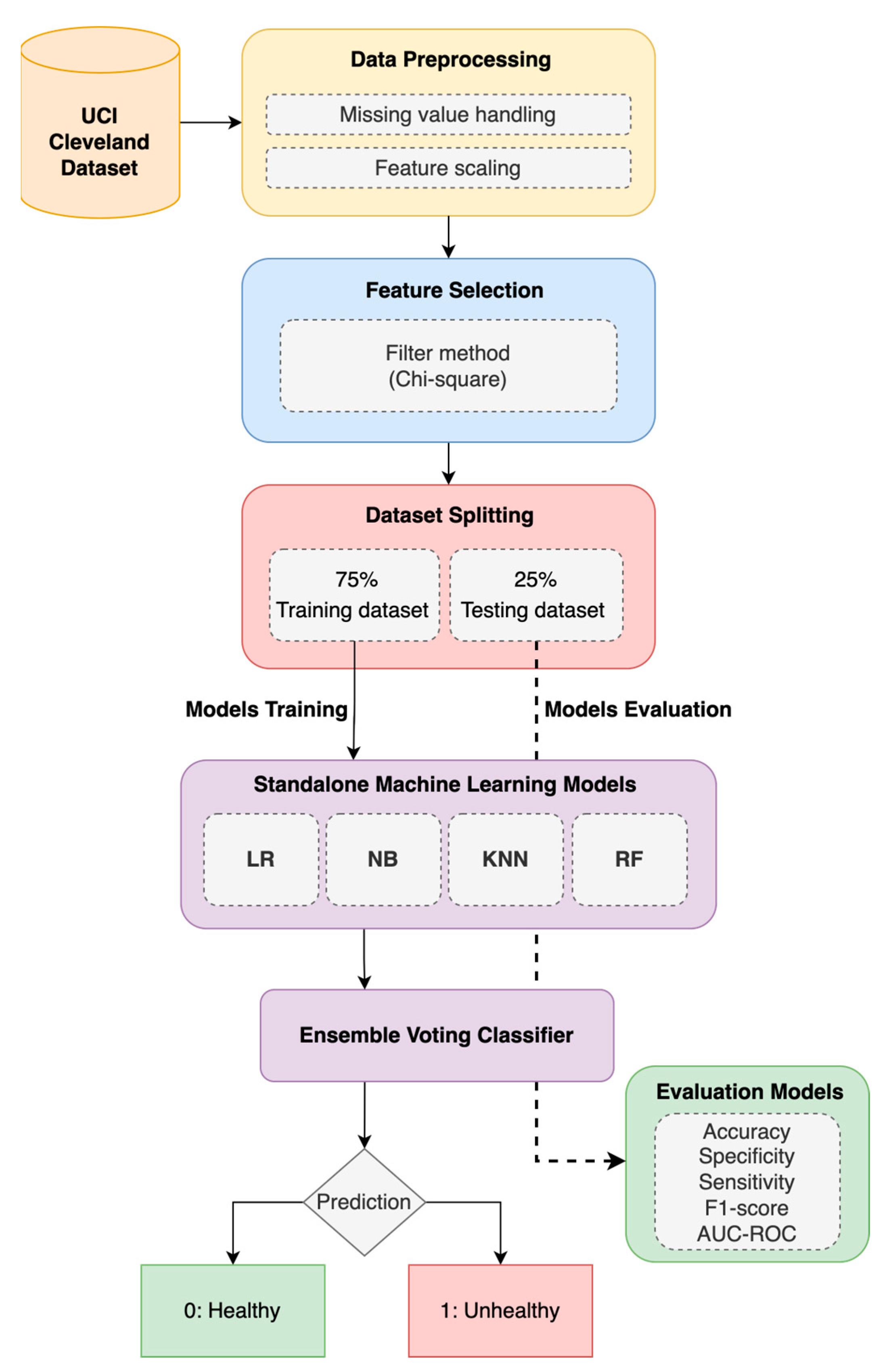
Figure 1. An overview of the overall operation of the proposed system.
Computers 13 00126 g001
Figure 2. Features’ importance in prediction, according to their chi-square scores.
Computers 13 00126 g002
Figure 3. Prediction accuracy.
Computers 13 00126 g003
Figure 4. Other metrics before feature selection.
Computers 13 00126 g004
Figure 5. Other metrics after feature selection.
Computers 13 00126 g005
Figure 6. ROC–AUC chart for base classifiers and voting ensemble classifier: (a) Before feature selection; (b) after feature selection.
Computers 13 00126 g006
Figure 7. Confusion matrix analysis before applying the chi-square feature selection algorithm: (a) Logistic regression (LR); (b) ensemble voting.
Computers 13 00126 g007
Figure 8. Confusion matrix analysis after applying the chi-square feature selection algorithm: (a) Logistic regression (LR); (b) ensemble voting.
Computers 13 00126 g008
Table 1. Cleveland dataset attributes [31].
NameTypeDescription
AgeNumberAge of person in years
SexCategory1 for Male and 0 for Female
CpCategoryChest pain type (4 for asymptomatic, 3 for non-anginal pain, 2 for atypical angina, and 1 for typical angina)
TrestbpsNumberBlood pressure in (mmHg)
CholNumberCholesterol in (mg/dL)
FbsCategoryMore than 120 mg/dL of fasting blood sugar (no = 0, yes = 1)
RestecgCategoryECG results (left ventricular hypertrophy = 2, ST-T wave abnormality = 1, normal = 0)
ThalachNumberheart rate
ExangCategoryAngina induced by exercise (yes = 1, no = 0)
OldpeakNumberST segment depression induced by exercise
SlopeCategorySloping of peak exercise ST segment (3 for downsloping, 2 for flat, 1 for upsloping)
CaCategoryThe total number of vessels that were colored via fluoroscopy
ThalCategoryResult of thallium stress test (reversible defect = 7, fixed = 6, normal = 3)
NumCategoryStatus of cardiac disease (0 if the diameter narrowing is less than 50%, 1 if it is greater than 50%)
Table 2. The chi-square test score calculation [47].
Class (Positive)Class (Negative)Total
When feature  x i  is presentabm = a + b
When feature  x i  is absentcdt – m = c + d
Totalp = a + ct – p = b + dt
Table 3. Evaluation of base classifiers and voting ensemble classifier performance without FS.
MethodTotal FeaturesAcc (%)Sen (%)Spe (%)F1-Score (%)
LR1385.5385.5385.5385.53
RF1385.5285.5285.5285.52
NB1381.5881.5881.5881.58
KNN1382.8982.8982.8982.89
Proposed Voting Ensemble1386.8486.8486.8486.84
Table 4. Evaluation of base classifiers and voting ensemble classifier performance with FS.
MethodTotal FeaturesAcc (%)Sen (%)Spe (%)F1-Score (%)
LR589.47389.47389.47389.473
RF588.15788.15788.15788.157
NB581.8581.8581.8581.85
KNN585.5385.5385.5385.53
Proposed Voting Ensemble592.1192.1192.1192.11
Table 5. A comparison of our proposed enhanced CVD detection system with the existing state-of-the-art methods.
WorkYearDatasetFeature Selection MethodClassifierNo. of Selected
Features
Accuracy
[20]2019ClevelandFeature SelectionBagging, Boosting, Voting Ensemble
(NB, RF, Bayes net, c4.5, MLP, PART)
97.26%
increase
[9]2019ClevelandExtra Tree ClassifierVoting, Bagging Ensemble
(DT, LR, ANN, KNN, NB)
-87.78%
[17]2019ClevelandFeature SelectionVoting Ensemble
(SVM, NB, LR)
684.79%
[24]2020Cleveland-Voting Ensemble ML (RF, SVM, KNN)
Voting Ensemble DL (LSTM, GRU)
-75–86%
[22]2020Cleveland-Voting Ensemble
(SVM, ANN, DT)
-87.3%
[21]2020ClevelandCFS with PSOStacked Ensemble
(RF, GBM, XGB)
785.71%
[23]2021Cleveland-Voting Ensemble
(NB, SVM, DT, NN, MLP, SLP)
-83%
[25]2021Cleveland-Voting Ensemble
(SVM, NB, ANN)
-87.05%
[16]2022ClevelandChi-square
and RFE
Voting Ensemble
(CART, GBM, Adaboost)
787%
[19]2022Cleveland-Voting Ensemble
(RF, KNN, DT, XGB, DNN, KDNN)
-88.70%
Proposed2024ClevelandChi-squareML Voting Ensemble
(NB, LR, RF, KNN)
592.11%
Disclaimer/Publisher’s Note: The statements, opinions and data contained in all publications are solely those of the individual author(s) and contributor(s) and not of MDPI and/or the editor(s). MDPI and/or the editor(s) disclaim responsibility for any injury to people or property resulting from any ideas, methods, instructions or products referred to in the content.