Article

Dealing with Class Overlap Through Cluster-Based Sample Weighting

by
Patrick Thiam
1,2,*,
Friedhelm Schwenker
2,*,† and
Hans Armin Kestler
1,†
1
Institute of Medical Systems Biology, Ulm University, Albert-Einstein-Allee 11, 89069 Ulm, Germany
2
Institute of Neural Information Processing, Ulm University, James-Franck-Ring, 89081 Ulm, Germany
*
Authors to whom correspondence should be addressed.
These authors contributed equally to this work.
Computers 2025, 14(11), 457; https://doi.org/10.3390/computers14110457
Submission received: 22 September 2025 / Revised: 15 October 2025 / Accepted: 20 October 2025 / Published: 24 October 2025
(This article belongs to the Special Issue Multimodal Pattern Recognition of Social Signals in HCI (2nd Edition))

Abstract

The classification performance of an inference model trained in a supervised manner depends substantially on the size and quality of the labeled training data. The characteristics of the underlying data distribution significantly impact the generalization ability of a trained model, particularly in cases where some class overlap can be observed. In such cases, training a single model on the entirety of the labeled data can result in an increase in the complexity of the resulting decision boundary, leading to over-fitting and consequently to some poor generalization performance. In the current work, a cluster-based sample weighting approach is proposed in order to improve the generalization ability of a classification model while dealing with such complex data distributions. The approach consists of first performing a clustering of the training data and subsequently optimizing cluster-specific classification models, using a weighted loss based on the samples-to-cluster-center distances. An unseen sample is first assigned a cluster and subsequently classified based on the model specific to its assigned cluster. The proposed approach was evaluated on three different pain recognition datasets, and the performed evaluation showed that the approach is not only able to attain state-of-the-art classification performances but also systematically outperforms its single model counterpart.

1. Introduction

Class overlap occurs when samples stemming from different classes share similar feature values, therefore resulting into a nearly impossible class discrimination. This is characterized by instances of different classes sharing common regions and being intertwined in the feature space, hence the discrimination between the different classes in those regions becoming nearly impossible. Consequently, optimizing an inference model on a dataset characterized by overlapping classes usually results in the generation of a complex decision boundary that eventually leads to over-fitting and consequently poor generalization performance [1,2,3]. Sample weighting constitutes one of the most prominent approaches designed to address class overlap. It consists of assigning weights to each sample of the training data according to its impact on the generalization ability of the designed classifier (or its relative importance) and solving the underlying optimization problem with the resulting weighted loss function.
Obviously, the main challenge relative to this specific approach consists in defining relevant sample weights or designing an approach to generate the sample weights in such a way that there is a positive impact on the generalization ability of the designed classifier. In recent years, various approaches, stemming from diverse areas such as meta-learning [4] or evolutionary algorithms [5], have been designed and proposed to tackle this specific issue. Ren et al. [6] proposed a meta-learning algorithm that learns to dynamically assign weights to training instances according to their gradient directions. However, the proposed approach relies on a clean unbiased validation set (an additional dataset from the same classification task not displaying any form of class overlap) in order to effectively optimize the neural network generating the sample weights. Such a dataset is usually not available in a real setting and must therefore be generated artificially, hence introducing bias into the whole classification task. A similar meta-learning approach was proposed by Shu et al. [7], and consists of an adaptive sample weighting strategy with the goal of automatically learning an explicit weighting function in the form of a multi-layer perceptron (MLP) from the training data. This MLP is referred to as a meta-weight-net (MW-Net) and consists of a single hidden layer. Similarly to the approach proposed by Ren et al. [6], the optimization of the MW-Net also relies on a clean and unbiased validation set, and thus this approach suffers from the same drawbacks in a real setting.
Meanwhile, Cui et al. [8] proposed an ensemble learning approach named cluster-based intelligence ensemble learning (CIEL). This approach consists in optimizing a set of cluster-specific classification models and performing a weighted aggregation of the output of the generated ensemble in order to perform the classification task. The parameters of the algorithm (clustering approaches, classification models, clustering parameters, classification parameters, and aggregation strategies and parameters) are simultaneously optimized using a particle swarm optimization (PSO) algorithm [9]. This yields a large amount of parameters being optimized, resulting in a computationally expensive and slow optimization approach (according to the size and nature of the classification task). Santiago et al. [10] propose a new optimization strategy called learning optimal sample weights (LOW) in order to dynamically train the parameters of a deep neural network while simultaneously optimizing the sample weights using the available training data. The approach aims to provide a substantially greater decrease in the loss function at each gradient descent step by adaptively optimizing the samples weights during the training process. Shu et al. [11] proposed a further improvement of the MW-Net approach called the class-aware meta-weight-net (CMW-Net). In contrast to the MW-Net, the CMW-Net consists in considering each class of the underlying classification task as a single learning task and optimizing sample-specific weights within each class separately based on each classes specific data distribution and bias characteristics. This is done in order to deal with the heterogeneous data bias observed with large-scale datasets that negatively impacts the performance of the MW-Net approach. Therefore, the original MW-Net is extended with an additional branch that integrates class-specific feature knowledge into the whole architecture, enabling the network to generate class-specific sample weights.
Similarly to the work presented by Cui et al. [8], the current work explores the idea of separating the dataset into a set of distinctive and non-overlapping clusters and then performing the optimization of cluster-specific inference models. Thereby, the complexity of the classification models can be significantly reduced. However, instead of the aggregation of the output of the trained cluster-specific models being performed to classify unseen samples, cluster-specific classification is performed. More precisely, unseen samples are first assigned a cluster, and the corresponding cluster-specific classification model is used to perform the classification task. Moreover, in order to handle the class imbalance that can occur due to the clustering process, a cluster-based sample weighting approach is proposed in order to perform the optimization of the cluster-specific classification models. This approach consists in weighting each sample of the training data according to its distance to the current cluster center in the feature space. The generated weights are subsequently used to perform the optimization of the cluster-specific classification model through a weighted loss function. The remainder of the work is organized as follows: the proposed approach is described in Section 2, followed by a description of the datasets and the designed performance assessment experiments in Section 3. A description of the results of the performed assessment is given in Section 4, followed by a discussion of the findings in Section 5. Finally, a summary of the main findings and description of some potential future work are provided in Section 6.

2. Proposed Approach

The proposed approach (depicted in Figure 1) consists of three specific and subsequent processes:
  • A latent space is generated using feature learning; this process is undertaken in order to reduce the dimensionality of the input data, which is crucial for the extraction of meaningful clusters; moreover, feature learning is performed in such a way that the knowledge relevant for the classification task at hand is preserved within the latent space.
  • Data clustering is performed within the generated latent space; each cluster is characterized by a cluster center and a spread that is subsequently used to define the weights of each sample; more specifically, each sample is weighted according to its distance to each of the cluster centers; this is done in order to avoid the negative effects of any form of class imbalance within each clusters, which could impact the performance of the subsequently trained classification models.
  • Cluster-specific classification models are optimized using a weighted loss function; the weights used for the optimization of each model correspond to the cluster related sample-specific weights, defined using a specific weighting function.
During the inference of unseen data instances, a sample is first projected into the latent space before being subsequently assigned a specific cluster. The inference is finally performed based on the corresponding optimized cluster-specific classification model.

2.1. Feature Learning

Feature learning is performed using a predefined deep denoizing convolutional auto-encoder (DDCAE) [12]. Similarly to an auto-encoder (AE) [13,14], a DDCAE consists of an encoder and a decoder, with both the encoder and the decoder being deep convolutional neural networks (DCNNs). The encoder projects its input into a low-dimensional latent space, while the decoder generates an output based on the corresponding latent representation. Moreover, the input of the encoder consists of a corrupted or altered input signal, and the decoder performs the reconstruction of the original and unaltered signal. The whole model is therefore optimized to reduce the reconstruction error between the decoder’s output and the original unaltered input signal. This results in a robust bottleneck representation that can subsequently be used for further tasks. The model is extended by applying an implicit rank-minimizing (IRM) approach proposed by Jing et al. [15] in order to reduce the rank of the covariance matrix of the latent representation, thus substantially removing the amount of noise and redundancy within the generated latent space. This is done by inserting a fixed number of extra linear layers between the encoder and the decoder, resulting into an IRM-DDCAE model. Therefore, given a set of training data T = { x i , y i | x i X R u × v , y i { 1 , 2 , , c } } i = 1 n (c depicting the number of classes), a set of altered input data is first generated: X ^ = { x ^ i , j X R u × v | 1 i n } j = 1 m (m representing the total amount of types of modifications (or noises) applied to the unaltered input signal). The noisy signals are subsequently fed into the encoder to generate the corresponding latent representations: h i , j = f θ x ^ i , j ( θ represents the set of weights specific to the encoder to be optimized, including the linear layers in the case of an IRM-DDCAE). The resulting latent representations are subsequently fed into the decoder to generate an output: x ˜ i , j = g ϕ ( h i , j ) ( ϕ represents the set of weights specific to the decoder to be optimized). The whole model is subsequently optimized based on the mean squared error (MSE) between the decoder’s output ( x ˜ i , j ) and the unaltered input signal ( x i ):
E = 1 n i = 1 n j = 1 m x i x ˜ i , j 2 2

2.2. Cluster-Based Sample Weighting (CbSW)

Subsequently, the training data is projected into the generated latent space by using the trained encoder: x i X , h i = f θ ( x i ) . The resulting data distribution in the latent space is partitioned using the K-means algorithm [16,17] (with K representing the amount of clusters to be created). It should be noted that other clustering algorithms (e.g., constrained clustering with complex cluster structure (C4S) [18]) can be used at this point. However, K-means is used due to both its simplicity and computational efficiency. Subsequently, each instance’s projection in the latent space h i is weighted according to its distance to each cluster center z k ( k { 1 , 2 , , K } ), as follows:
w i , k = a + 1 , if h i k -th cluster a + 1 1 + h i z k 2 otherwise
where a 0 , 1 . This weighting function assigns an identical weight to any instance assigned to the k-th cluster. The remaining instances not assigned to the k-th cluster are assigned weights inversely proportional to the distance from the instance to the cluster’s center z k (the further the instance, the lower the weight). By doing so, all training instances can subsequently be used to optimize a classification model specific to the k-th cluster with the relative importance of each sample reflected by its assigned weight. Moreover, any issue related to the class imbalance that might occur within a single cluster is herewith handled since the entirety of the training data is used for the optimization of the model (ensuring that all the classes are seen by each cluster-specific classification model).

2.3. Cluster-Specific Model Optimization

Following the generation of the cluster-specific sample weights, a single classification model is optimized for each one of the K clusters to perform the classification of each assigned instance. In the case of a neural network, the k-th classifier (classifier specific to the k-th cluster) is optimized based on the following weighted loss function:
Loss = 1 n i = 1 n w i , k × L y i , y ˜ i
where y ˜ i is the output of the classifier, and L y i , y ˜ i is a fixed loss function.
During inference, an unseen sample is first projected into the latent space using the trained encoder ( f θ ) and subsequently assigned a cluster based on the trained K-means model. Finally, the classification is performed using the model specific to the assigned cluster.

3. Experiments

In order to perform the assessment of the proposed approach, 3 datasets collected in order to develop automatic pain recognition systems based on audiovisual and bio-physiological signals were selected. Pain recognition is known to be a very cumbersome classification task due to its highly subjective nature [19,20]. Pain perception and pain expression vary greatly from one individual to the next and are significantly influenced by factors such as an individual’s age, level of fitness, or psychological profile. Thus, each individual is characterized by some highly heterogeneous data distribution. Therefore, a collection of data stemming from different individuals depicts significant class overlap. In the current section, a short description of the datasets is provided, followed by a description of the experimental settings and assessment procedures.

3.1. BioVid Heat Pain Database

The BioVid Heat Pain Database [21] is a multi-modal database consisting of two datasets (BioVid Part A and BioVid Part B). Both datasets consist of healthy participants subjected to 4 levels of gradually increasing and individually calibrated thermal pain elicitation. Different modalities were recorded during the experiments leading to the creation of both datasets, including video streams, electrodermal activity (EDA), electrocardiography (ECG), and electromyography (EMG) (corrugator, zygomaticus, and trapezius) signals. Each single level of pain elicitation was randomly elicited a total of 20 times, with each elicitation lasting 4 seconds (sec), followed by a recovery phase of randomized duration (lasting between 8 and 12 s). During this recovery phase, a baseline temperature T 0 of 32 °C was applied. The BioVid Part A dataset consists of 87 participants, while the BioVid Part B dataset consists of 86 participants. In this specific setting, the classes consists of the baseline level and the 4 levels of pain elicitation ( T 0 , T 1 , T 2 , T 3 , T 4 ). Therefore, the BioVid Part A dataset consists of a total of 87 × 5 × 20 = 8700 samples, while the BioVid Part B consists of a total of 86 × 5 × 20 = 8600 samples.

3.2. SenseEmotion Dataset

Similarly to the BioVid Heat Pain Database, the SenseEmotion Dataset [22] consists of 45 healthy individuals subjected to 3 levels of individually calibrated and gradually increasing thermal pain elicitation ( T 1 , T 2 , T 3 ) and a baseline level T 0 set identically for all participants to 32 °C. The modalities recorded during the performed experiments consist of audio signals; video streams; the trapezius EMG signal; and the respiration, ECG, and EDA signals. Each level of pain elicitation was randomly elicited a total of 30 times with a pause of about 8 to 12 s following each elicitation. The performed experiments consist of two 40-minute (min) sessions, during which the piece of hardware used to perform the thermal pain elicitations was attached to a specific forearm (once on the right forearm and once on the left forearm). The calibration of the temperatures of elicitation and the thermal elicitation procedure were carried out identically to those of the BioVid Heat Pain Database. Due to technical issues during the experiments, 5 participants were excluded from the dataset because of missing or erroneous data. The evaluation was therefore performed on a reduced subset consisting of 40 participants and a dataset consisting of a total of 40 × 4 × 30 × 2 = 9600 samples.

3.3. Data Preprocessing

For the current work, all evaluation experiments were performed uniquely using the EDA modality. This was done in order to clearly assess the performance of the proposed approach since previous works in the domain of thermal induced pain recognition have shown EDA to significantly outperform other forms of audiovisual and physiological modalities [23,24,25]. Furthermore, the classification task consisted of discrimination between the baseline and the highest level of pain elicitation ( T 0 vs. T 4 for the BioVid datasets; T 0 vs. T 3 for the SenseEmotion dataset) in order to generate unambiguous classification results and enable the comparison of the proposed approach with previous work. The resulting data was preprocessed as described in [26]. The raw signals were preprocessed by applying a 3rd-order low-pass Butterworth filter with a cut-off frequency of 0.2 Hz (Hertz), followed by reducing the sampling rate to 256 Hz in order to reduce the amount of computational requirements. The resulting filtered signals were subsequently segmented, and each segment with its corresponding level of pain elicitation was used to perform the classification task. In the case of the BioVid datasets, the segments corresponded to windows of length 4.5 s with a shift of 4 s from the elicitation onset. In the case of the SenseEmotion dataset, the segments corresponded to windows of length 6.5 s with a similar shift of 4 s from the elicitation onset. Therefore, each signal consisted of a 1-dimensional array of size l = 4.5 × 256 = 1152 for the BioVid datasets and l = 6.5 × 256 = 1664 for the SenseEmotion dataset. The data used for the assessment of the approach can be summarized in each case as follows:
  • BioVid Part A: T = { x i , y i | x i R 1 × 1152 , y i { 0 , 4 } } i = 1 3480 ;
  • BioVid Part B: T = { x i , y i | x i R 1 × 1152 , y i { 0 , 4 } } i = 1 3440 ;
  • SenseEmotion: T = { x i , y i | x i R 1 × 1664 , y i { 0 , 3 } } i = 1 4800 .

3.4. Experimental Settings

A leave-one-subject-out (LOSO) cross-validation evaluation was performed on each dataset in order to assess the proposed approach. More specifically, the data specific to each single participant was used once to evaluate the performance of the optimized architecture and was never seen during the training process, while the data specific to the remaining participants was used to optimize the whole architecture (i.e., DDCAE, K-means model and classification model). The performance measures used to conduct the assessment were defined as follows:
Accuracy = t p + t n t p + t n + f p + f n
(tp: true positives; tn: true negatives; fp: false positives; fn: false negatives).
F 1 -Score = 2 × P r e c i s i o n × R e c a l l P r e c i s i o n + R e c a l l
where P r e c i s i o n = t p t p + f p and R e c a l l = t p t p + f n .
The DDCAE model designed for the feature learning step is an extension of the architecture presented in [27]. The encoder consists of a series of convolutional blocks as depicted in Figure 2: each block consists of a 1-dimensional convolutional layer, followed by a batch normalization (BN) layer and an activation layer. Throughout the work, the exponential linear unit (ELU) function [28] is used as activation function unless indicated otherwise. The output is subsequently fed into a residual spatial attention module as proposed in [26,29], followed by a max pooling layer and finally a dropout layer. The size of the kernel of the convolutional layer is set to 3 with a stride of 1, the size of the pooling layer is set to 2 with a stride of 2, and the dropout rate is set to 0.3 .
The decoder consists of a series of transposed convolutional blocks: each block consists of a 1-dimensional transposed convolutional layer, followed by a batch normalization layer and an activation layer successively. The last layer of the decoder consists of a linear convolutional layer. The kernels’ parameters are set in such a way that the dimensionality of the resulting output signal is equal to the dimensionality of the input signal. A summary of both architectures can be seen in Table 1. The IRM-DDCAE consists of the same architecture with an additional set of 4 fully connected linear layers (without any bias term or activation function) added successively between the encoder output and the decoder input while preserving the exact same dimensionality as that of the encoder output.
Due to the huge amount of parameters to be optimized, data augmentation was performed. It was conducted by shifting the windows of segmentation forward and backward through time, with small shifts of 250 milliseconds (ms) and a total window shift of 1 s in each direction, starting from the initial position chosen for the segmentation described earlier. Furthermore, 3 categories of noise were used in order to generate the altered input signals of the decoder: Random Gaussian noise injection with the following parameters set empirically: mean set to 0 and standard deviation set to 0.005 ; random signal permutation; random time masking with varying window sizes. The defined models (DDCAE and IRM-DDCAE) were trained using the adaptive moment estimation (Adam) [30] optimization algorithm for a total of 30 epochs, with a fixed learning rate set to 10 5 . The batch size was set to 40 for both BioVid datasets and to 60 for the SenseEmotion dataset.
Following the optimization of the DDCAE (resp. IRM-DDCAE), the feature representations of the training set were extracted using the trained encoder. Subsequently, a fixed number of clusters was selected by performing an evaluation of the sample weighting approach using an ensemble of k cluster-specific classifiers on the validation set (with k { 2 , 3 , 4 , 5 , 6 , 7 , 8 , 9 , 10 } ). The weighting function’s parameter a was set empirically throughout the performed experiments as follows: a = 0.1 . This was done in order to avoid having extremely low weights for samples located far away from the current cluster center, resulting in those samples having no impact at all on the decision boundary of the trained classifier. The impact of such samples should be reduced and not removed. The best performing ensemble of classifiers (best k value) was subsequently selected to perform the classification task on the defined test set. The architecture of each classifier consisted of 2 dense blocks (with a dense block consisting of a fully connected layer, followed by an activation layer and a dropout layer) with 256 and 64 units respectively, followed by a final fully connected layer (with 2 units) and an activation layer with a softmax activation function. The dropout rate was set to 0.3 , and each classifier was trained using the Adam optimization algorithm for a total of 100 epochs. The learning rate was set to 10 5 , and the batch size for all datasets was set to 100. The classifiers were trained with the categorical cross-entropy loss. The implementation and the evaluation of the proposed approach was performed with the libraries Tensorflow [31] (version: 2.16.1), Keras [32] (version: 3.11.2), and Scikit-learn [33] (version: 1.6.1).

4. Results

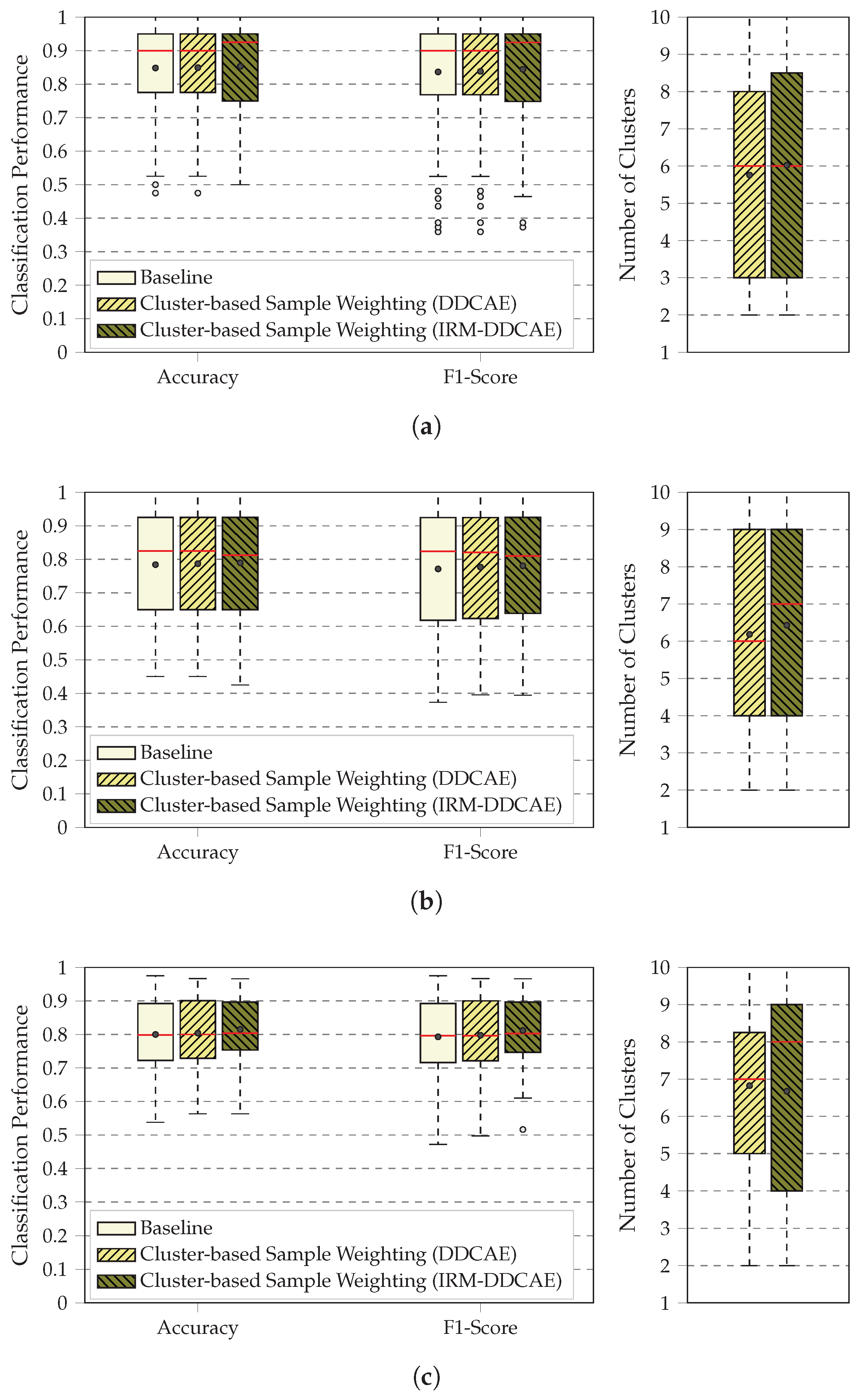
The first conducted experiment consisted of evaluating and comparing the performance of the proposed approach with that of a single classifier optimized using the latent representation stemming from the DDCAE (Baseline). At the same time, the impact of the implicit rank-minimizing (IRM) extension was evaluated by comparing the performance of the sample weighting approach based on the DDCAE latent representation and the IRM-DDCAE latent representation. The results are summarized in both Figure 3 and Table 2. In Figure 3, the results depict a high variance which is typical to pain recognition tasks and reflects the subjective nature of pain. Moreover, the DDCAE is able to extract meaningful features in an unsupervised manner, which can subsequently be used in order to perform the classification task at a satisfactory extent. The proposed sample weighting approach is also able to further improve the classification performance for each dataset, based on a median value of k = 6 clusters for both BioVid datasets and k = 7 clusters for the SenseEmotion dataset. The sample weighting approach based on the IRM-DDCAE latent representation outperforms both its DDCAE counterpart as well as the baseline approach, thus showing that a better latent representation can subsequently improve the performance of the whole architecture.
This is better seen in Table 2: concerning both BioVid datasets, the approach based on the IRM-DDCAE latent representation outperforms the other approaches in terms of accuracy and F1-score, with a median of k = 6 clusters for the BioVid Part A dataset and k = 7 clusters for the BioVid Part B dataset. This performance improvement is even significant in the case of the SenseEmotion dataset with a median number of k = 8 clusters.
Based on these results, a further experiment was conducted in order to assess the relevance of the information injected into the whole architecture through the performed clustering of the latent space. Based on the latent representation stemming from the IRM-DDCAE, a particle swarm optimization sample weighting (PSOSW) approach was designed in order to generate sample-specific weights without any clustering phase being involved. Each particle in the PSOSW approach is a vector consisting of the weights of the samples belonging to the training set. From these weights (or from each particle), a classifier with the same architecture and optimization parameters as described in Section 3 can be trained with the resulting weighted categorical cross-entropy loss. The fitness function used to drive the exploration (resp. exploitation) of the PSO algorithm is therefore the classification performance in terms of accuracy on a validation set. The PSO algorithm is run for a total number of 20 epochs (time steps), with a total of 10 particles and a neighborhood size of 5 (with the neighborhoods formed by using the Euclidean distance between particles). Given the position of the i-th particle s i t as well as its velocity v i t at the time step t, the following equations are used to actualize both parameters at the next time step t + 1 :
v i t + 1 = w t × v i t + c 1 × r 1 × p i t s i t + c 2 × r 2 × g i t s i t
s i t + 1 = s i t + v i t + 1
where p i t and g i t denote, respectively, the personal and global best positions of the i-th sample at the time step t; r 1 and r 2 are random parameters selected at each time step from a uniform distribution within the range [ 0 , 1 ] ; and both cognitive and social acceleration constants c 1 and c 2 are set to a fixed value of 2. In order to avoid any premature convergence and balance the optimization process between exploration and exploitation as proposed in [34,35], the inertia weight parameter w t is actualized at each time step t using the following equation:
w t = w m a x w m i n × t m a x t t m a x + w m i n
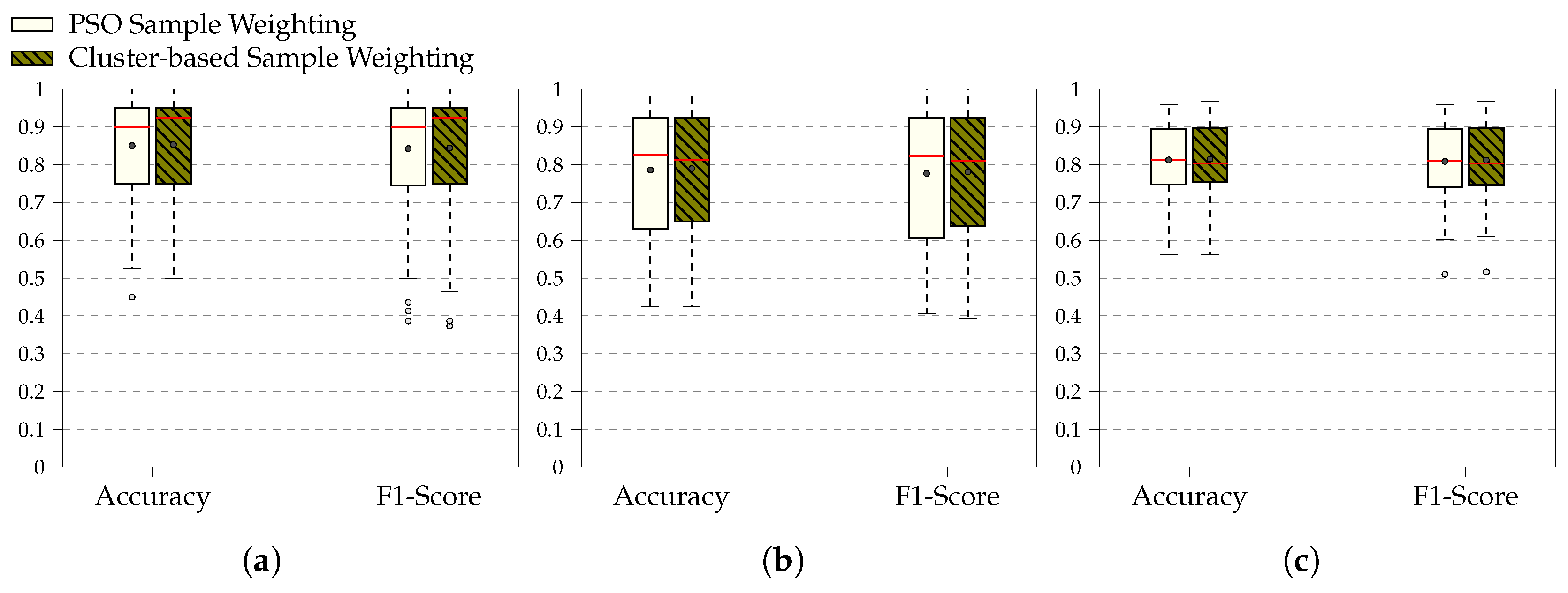
where w m a x = 2 , w m i n = 0.4 , and t m a x = 20 . The initial values of each particle’s coordinates (samples’ weights) are randomly selected in the range [ a , a + 1 ] (with a = 0.1 ). The results of the optimization, including the comparison to the cluster-based approach, can be seen in both Table 3 and Figure 4. Even though the results appear similar at first glance, the cluster-based approach in these settings outperforms the PSO-based approach in terms of averaged accuracy and F1-score for each single dataset. Therefore, it is believed that the resulting clustering structure plays a very important role in the sample weighting approach and can be further investigated in order to improve the performance of the whole classification architecture.

5. Discussion

The findings of the performed experiments point to the fact that relevant feature representations can be learned in an unsupervised manner, even for complex classification tasks. The classification model trained on the latent representation stemming from the encoder of the DDCAE is able to perform the classification task at a satisfactory extent. Moreover, the integration of information represented as sample-specific weights helps further improve the overall classification performance of the designed architecture. Therefore, it is believed that not every available sample in the training set is relevant to the task at hand and should be weighted accordingly. Thus, cluster-based sample weighting is considered to be a sound approach, particularly when confronted with overlapping classes. Further improvement of the overall classification performance (as well as significant performance improvement in some cases) can be achieved through the IRM-DDCAE approach. This points to the fact that the underlying latent representation plays a significant role when it comes to applying the cluster-based sample weighting approach. Improving the latent representation can help define relevant clusters withing the feature space and subsequently boost the overall performance of the classification architecture.
Additionally, the comparison of the performance between the IRM-DDCAE cluster-based sample weighting approach and a PSO sample-weighting approach (which optimizes the weights of the training samples without involving any form of clustering) also points to the relevance of the performed clustering. The information stemming from the clusters and integrated into the sample-weighting approach improves the overall performance of the classification architecture. Finally, as can be seen in Table 4, the approach is able to attain state-of-the-art classification performances in comparison to previous work. The best-performing approaches rely on Transformer architectures [36]; hence, future work should involve extending the proposed IRM-DDCAE with a corresponding Transformer scheme in order to further improve the data distribution of the resulting latent space.
Since the proposed approach is built in a modular manner, it offers some flexibility in its overall design in comparison to a typical end-to-end approach. Different types of deep learning approaches (e.g., Transformer auto-encoder, transfer learning) can be used to generate the latent space, or hand-crafted features can be directly used to perform both clustering and classification tasks. Different forms of classifiers such as linear support vector machines or decision trees can be used to perform the inference instead of neural networks. Moreover, parallelization can be applied to speed up the optimization of the models as well as the inference time. This flexibility can be exploited in order to further improve the performance of the proposed approach. Based on recent advancements in graph-neural-network (GNN)-based sample modeling [37,38], it is believed that further performance improvement could be achieved by adapting such methods to the proposed approach.
Furthermore, since the main assumption behind the K-means clustering approach is the spherical and isotropic shape of the clusters in the feature space, an exploration of other clustering approaches (with the corresponding weighting function) should be performed because this assumption does not hold for every dataset. It is hoped that exploring further clustering algorithms can potentially improve the performance of the whole architecture with consideration to specific characteristics of the underlying data distribution.
Table 4. Classification performance in comparison to previous work. Dataset: BioVid Part A. Modality: EDA. Evaluation: leave one subject out (LOSO). Classification task: T 0 vs. T 4 .
ApproachAccuracy (%)
Werner et al. [39]: Random Forests Classifier with 100 Trees 71.90
Kächele et al. [40]: Random Forests Classifier with 500 Trees 81.90
Thiam et al. [27]: 1-Dimensional Convolutional Neural Network (1-D CNN) 84.57
Phan et al. [41]: 1-D CNN & Bidirectional Long Short-Term Memory (BiLSTM) 84.80
Lu et al. [42]: Multiscale Convolutional Networks & Squeeze-Excitation Residual Networks & Transformer Encoder (PainAttnNet) 85.56
Li et al. [43]: Multi-Dimensional Temporal Convolutional Network & Activate Channels Feature Network & Cross-Attention Temporal Convolutional Network (EDAPainNet) 86.21
Current Approach: Cluster-based Sample Weighting (IRM-DDCAE) 85.32

6. Conclusions

The current work has shown that given a specific data distribution, all samples are not equally relevant for an underlying classification task. Learning to weight these samples appropriately helps to deal with the issues inherent to class overlapping and thereby provides some significant overall classification performance improvement. The proposed cluster-based sample weighting is able to attain state-of-the-art classification performances and still presents some potential for further improvement. Improving the data distribution of the underlying latent space and designing an appropriate sample weighting in combination with the chosen clustering approach constitute relevant topics for future works.

Author Contributions

Conceptualization, P.T.; methodology, P.T.; software, P.T.; validation, P.T.; formal analysis, P.T.; investigation, P.T., H.A.K., and F.S.; resources, H.A.K. and F.S.; data curation, P.T.; writing—original draft preparation, P.T.; writing—review and editing, P.T., H.A.K., and F.S.; visualization, P.T.; supervision, H.A.K. and F.S.; project administration, H.A.K.; funding acquisition, H.A.K. All authors have read and agreed to the published version of the manuscript.

Funding

HAK acknowledges funding from the German Science Foundation (DFG, SFB 1506; grant no. 450627322) and BMFTR (Project Private Aim; grant no. 01ZZ2316N and CALM-QE 01ZZ2318I).

Data Availability Statement

The BioVid Heat Pain Database (including both Part A and Part B) is available for non-commercial research only. The database can be accessed by sending a signed agreement form (available at https://www.nit.ovgu.de/BioVid.html (accessed on 3 September 2025)) to Sascha Gruss at sascha.gruss@uni-ulm.de. The SenseEmotion Dataset can be accessed by directly contacting Steffen Walter at steffen.walter@uni-ulm.de.

Conflicts of Interest

The authors declare no conflicts of interest.

Abbreviations

The following abbreviations are used in this manuscript:
MLPmulti-layer perceptron
MW-Netmeta-weight-net
CIELcluster-based intelligence ensemble learning
PSOparticle swarm optimization
LOWlearning optimal sample weights
CMW-Netclass-aware meta-weight-net
DDCAEdeep denoizing convolutional auto-encoder
AEauto-encoder
DCNNdeep convolutional neural network
IRMimplicit rank-minimizing
IRM-DDCAEimplicit rank-minimizing deep denoizing convolutional auto-encoder
BNbatch normalization
ELUexponential linear unit
MSEmean squared error
EDAelectrodermal activity
ECGelectrocardiography
EMGelectromyography
HzHertz
LOSOleave one subject out
CbSWcluster-based sample weighting
PSOSWparticle swarm optimization sample weighting
GNNsgraph neural networks

References

  1. Vuttipittayamongkol, P.; Elyan, E.; Petrovski, A. On the Class Overlap Problem in Imbalanced Data Classification. Knowl.-Based Syst. 2021, 212, 106631. [Google Scholar] [CrossRef]
  2. Soltanzadeh, P.; Feizi-Derakhshi, M.R.; Hashemzadeh, M. Addressing the Class-Imbalance and Class-Overlap Problems by a Metaheuristic-based Under-Sampling Approach. Pattern Recognit. 2023, 143, 109721. [Google Scholar] [CrossRef]
  3. Santos, M.S.; Abreu, P.H.; Japkowicz, N.; Fernández, A.; Santos, J. A Unifying View of Class Overlap and Imbalance: Key Concepts, Multi-View Paranoma, and Open Avenues for Research. Inf. Fusion 2023, 89, 228–253. [Google Scholar] [CrossRef]
  4. Thrun, S.; Pratt, L. Learning to Learn: Introduction and Overview. In Learning to Learn; Springer: Boston, MA, USA, 1998; pp. 3–17. [Google Scholar] [CrossRef]
  5. De Jong, K.A. Evolutionary Computation: A Unified Approach; The MIT Press: Cambridge, MA, USA, 2006; Available online: https://ieeexplore.ieee.org/servlet/opac?bknumber=6267245 (accessed on 22 October 2025).
  6. Ren, M.; Zeng, W.; Yang, B.; Urtasun, R. Learning to Reweight Examples for Robust Deep Learning. In Proceedings of the 35th International Conference on Machine Learning, Stockholmsmässan, Sweden, 10–15 July 2018; Volume 80, pp. 4334–4343. Available online: https://proceedings.mlr.press/v80/ren18a/ren18a.pdf (accessed on 22 October 2025).
  7. Shu, J.; Xie, Q.; Yi, L.; Zhao, Q.; Zhou, S.; Xu, Z.; Meng, D. Meta-Weight-Net: Learning an Explicit Mapping For Sample Weighting. In Proceedings of the 33rd International Conference on Neural Information Processing Systems, Vancouver, BC, Canada, 8–19 December 2019; Wallach, H., Larochelle, H., Beygelzimer, A., d’Alché-Buc, F., Fox, E., Garnett, R., Eds.; Curran Associates Inc.: Red Hook, NY, USA, 2019; Volume 32. Available online: https://proceedings.neurips.cc/paper_files/paper/2019/file/e58cc5ca94270acaceed13bc82dfedf7-Paper.pdf (accessed on 22 October 2025).
  8. Cui, S.; Wang, Y.; Yin, Y.; Cheng, T.; Wang, D.; Zhai, M. A Cluster-based Intelligence Ensemble Learning Method for Classification Problems. Inf. Sci. 2021, 560, 386–409. [Google Scholar] [CrossRef]
  9. Kennedy, J.; Eberhardt, R. Particle Swarm Optimization. In Proceedings of the ICNN’95—International Conference on Neural Networks, Perth, Australia, 25 November–1 December 1995; Volume 4, pp. 1942–1948. [Google Scholar] [CrossRef]
  10. Santiago, C.; Barata, C.; Sasdelli, M.; Carneiro, G.; Nascimento, J.C. LOW: Training Deep Neural Networks by Learning Sample Weights. Pattern Recognit. 2021, 110, 107585. [Google Scholar] [CrossRef]
  11. Shu, J.; Yuan, X.; Meng, D.; Xu, Z. CMW-Net: Learning a Class-Aware Sample Weighting Mapping for Robust Deep Learning. IEEE Trans. Pattern Anal. Mach. Intell. 2023, 45, 11521–11539. [Google Scholar] [CrossRef]
  12. Thiam, P.; Kestler, H.A.; Schwenker, F. Multimodal Deep Denoising Convolutional Autoencoders for Pain Intensity Classification based on Physiological Signals. In Proceedings of the 9th International Conference on Pattern Recognition Applications and Methods (ICPRAM), Valetta, Malta, 22–24 February 2020; INSTICC: Lisboa, Portugal; SciTePress: Setubal, Portugal, 2020; Volume 1, pp. 289–296. [Google Scholar] [CrossRef]
  13. Hinton, G.E.; Zemel, R.S. Autoencoders, Minimum Description Length and Helmholtz Free Energy. In Proceedings of the 7th International Conference on Neural Information Processing Systems NIPS’93, Denver, CO, USA, 29 November–2 December 1993; Morgan Kaufmann Publishers Inc.: San Francisco, CA, USA, 1993; pp. 3–10. Available online: https://proceedings.neurips.cc/paper/1993/file/9e3cfc48eccf81a0d57663e129aef3cb-Paper.pdf (accessed on 22 October 2025).
  14. Hinton, G.E.; Salakhutdinov, R. Reducing the Dimensionality of Data with Neural Networks. Science 2006, 313, 504–507. [Google Scholar] [CrossRef] [PubMed]
  15. Jing, L.; Zbontar, J.; LeCun, Y. Implicit Rank-Minimizing Autoencoder. In Proceedings of the 34th International Conference of Neural Information Processing Systems, Vancouver, BC, Canada, 6–12 December 2020; Curran Associates Inc.: Red Hook, NY, USA, 2020; pp. 14736–14746. Available online: https://proceedings.neurips.cc/paper/2020/file/a9078e8653368c9c291ae2f8b74012e7-Paper.pdf (accessed on 22 October 2025).
  16. MacQueen, J. Some Methods for Classification and Analysis of Multivariate Observations. In 5th Berkeley Symposium on Mathematical Statistics and Probability; Le Cam, L.M., Neyman, J., Eds.; University of California Press: Oakland, CA, USA, 1967; Volume 1, pp. 281–297. Available online: https://projecteuclid.org/ebooks/berkeley-symposium-on-mathematical-statistics-and-probability/Proceedings-of-the-Fifth-Berkeley-Symposium-on-Mathematical-Statistics-and/chapter/Some-methods-for-classification-and-analysis-of-multivariate-observations/bsmsp/1200512992 (accessed on 22 October 2025).
  17. Lloyd, S.P. Least Squares Quantization in PCM. IEEE Trans. Inf. Theory 1982, 28, 129–137. [Google Scholar] [CrossRef]
  18. Śmieja, M.; Wiercioch, M. Constrained Clustering with a Complex Cluster Structure. Adv. Data Anal. Classif. 2017, 11, 493–518. [Google Scholar] [CrossRef]
  19. Coghill, R.C.; McHaffie, J.G.; Yen, Y.F. Neural Correlates of Interindividual Differences in the Subjective Experience of Pain. Proc. Natl. Acad. Sci. USA 2003, 100, 8538–8542. [Google Scholar] [CrossRef]
  20. Nielsen, C.S.; Stubhaug, A.; Price, D.D.; Vassend, O.; Czajkowski, N.; Harris, J.R. Individual Differences in Pain Sensitivity: Genetic and Environment Contributions. Pain 2008, 136, 21–29. [Google Scholar] [CrossRef]
  21. Walter, S.; Gruss, S.; Ehleiter, H.; Tan, J.; Traue, H.C.; Crawcour, S.; Werner, P.; Al-Hamadi, A.; Andrade, A. The BioVid Heat Pain Database: Data for the Advancement and Systematic Validation of an Automated Pain Recognition System. In Proceedings of the 2013 IEEE International Conference on Cybernetics (CYBCO), Lausanne, Switzerland, 13–15 June 2013; pp. 128–131. [Google Scholar] [CrossRef]
  22. Velana, M.; Gruss, S.; Layher, G.; Thiam, P.; Zhang, Y.; Schork, D.; Kessler, V.; Gruss, S.; Neumann, H.; Kim, J.; et al. The SenseEmotion Database: A Multimodal Database for the Development and Systematic Validation of an Automatic Pain- and Emotion-Recognition System. In Proceedings of the Multimodal Pattern Recognition of Social Signals in Human-Computer-Interaction, Cancun, Mexico, 4 December 2016; Schwenker, F., Scherer, S., Eds.; Springer: Cham, Switzerland, 2017; pp. 127–139. [Google Scholar] [CrossRef]
  23. Pouromran, F.; Radhakrishnan, S.; Kamarthi, S. Exploration of Physiological Sensors, Features, and Machine Learning Models for Pain Intensity Estimation. PLoS ONE 2021, 16, e0254108. [Google Scholar] [CrossRef] [PubMed]
  24. Werner, P.; Lopez-Martinez, D.; Walter, S.; Al-Hamadi, A.; Gruss, S.; Picard, R.W. Automatic Recognition Methods Supporting Pain Assessment: A Survey. IEEE Trans. Affect. Comput. 2022, 13, 530–552. [Google Scholar] [CrossRef]
  25. Rojas, R.F.; Hirachan, N.; Brown, N.; Waddington, G.; Murtagh, L.; Seymour, B.; Goecke, R. Multimodal Physiological Sensing for the Assessment of Acute Pain. Front. Pain Res. 2023, 4, 1150264. [Google Scholar] [CrossRef] [PubMed]
  26. Thiam, P.; Hihn, H.; Braun, D.A.; Kestler, H.A.; Schwenker, F. Multi-Modal Pain Intensity Assessment Based on Physiological Signals: A Deep Learning Perspective. Front. Physiol. 2021, 12, 720464. [Google Scholar] [CrossRef]
  27. Thiam, P.; Bellmann, P.; Kestler, H.A.; Schwenker, F. Exploring Deep Physiological Models for Nociceptive Pain Recognition. Sensors 2019, 20, 4503. [Google Scholar] [CrossRef] [PubMed]
  28. Clevert, D.A.; Unterthiner, T.; Hochreiter, S. Fast and Accurate Deep Neural Network Learning by Exponential Linear Units (ELUs). In Proceedings of the 4th International Conference on Learning Representations, ICLR 2016, San Juan, Puerto Rico, 2–4 May 2016; Conference Track Proceedings. Available online: http://arxiv.org/abs/1511.07289 (accessed on 22 October 2025).
  29. Woo, S.; Park, J.; Lee, J.Y.; Kweon, I.S. CBAM: Convolutional Block Attention Module. In Proceedings of the 15th European Conference on Computer Vision (ECCV), Munich, Germany, 8–14 September 2018; Springer: Berlin/Heidelberg, Germany, 2018. Proceedings, Part VII. pp. 3–19. [Google Scholar] [CrossRef]
  30. Kingma, D.P.; Ba, J. Adam: A Method for Stochastic Optimization. In Proceedings of the 3rd International Conference on Learning Representations, ICLR 2015, San Diego, CA, USA, 7–9 May 2015; Conference Track Proceedings. Available online: https://arxiv.org/abs/1412.6980 (accessed on 22 October 2025).
  31. Abadi, M.; Barham, P.; Chen, J.; Chen, Z.; Davis, A.; Dean, J.; Devin, M.; Ghemawat, S.; Irving, G.; Isard, M.; et al. Tensorflow: A System for Large-Scale Machine Learning. In Proceedings of the 12th USENIX Symposium on Operating Systems Design and Implementation (OSDI 16), Savannah, GA, USA, 1–4 November 2016; pp. 265–283. Available online: https://www.usenix.org/system/files/conference/osdi16/osdi16-abadi.pdf (accessed on 22 October 2025).
  32. Chollet, F. Keras. 2015. Available online: https://keras.io (accessed on 3 September 2025).
  33. Pedregosa, F.; Varoquaux, G.; Gramfort, A.; Michel, V.; Thirion, B.; Grisel, O.; Blondel, M.; Prettenhofer, P.; Weiss, R.; Dubourg, V.; et al. Scikit-learn: Machine Learning in Python. J. Mach. Learn. Res. 2011, 12, 2825–2830. [Google Scholar]
  34. Shi, Y.; Eberhart, R.C. Parameter Selection in Particle Swarm Optimization. In Proceedings of the 7th International Conference on Evolutionary Programming, San Diego, CA, USA, 25–27 March 1998; Lecture Notes in Computer Science. Porto, V.W., Saravanan, N., Waagen, D., Eiben, A.E., Eds.; Springer: Berlin/Heidelberg, Germany, 1998; Volume 1447, pp. 591–600. [Google Scholar] [CrossRef]
  35. Arasomwan, M.A.; Adewumi, A.O. On the Performance of Linear Decreasing Inertia Weight Particle Swarm Optimization for Global Optimization. Sci. World J. 2013, 1, 860289. [Google Scholar] [CrossRef]
  36. Vaswani, A.; Shazeer, N.; Parmar, N.; Uszkoreit, J.; Jones, L.; Gomez, A.N.; Kaiser, L.; Polosukhin, I. Attention is All You Need. In Proceedings of the 31st International Conference on Neural Information Processing Systems NIPS’ 17, Long Beach, CA, USA, 4–9 December 2017; Guyon, I., Von Luxburg, U., Bengio, S., Wallach, H., Fergus, R., Vishwanathan, S., Garnett, R., Eds.; Curran Associates Inc.: Red Hook, NY, USA, 2017; Volume 30, pp. 6000–6010. Available online: https://proceedings.neurips.cc/paper_files/paper/2017/file/3f5ee243547dee91fbd053c1c4a845aa-Paper.pdf (accessed on 22 October 2025).
  37. Chen, Z.; Xiao, T.; Kuang, K.; Lv, Z.; Zhang, M.; Yang, J.; Lu, C.; Yang, H.; Wu, F. Learning To Reweight for Generalizable Graph Neural Networks. In Proceedings of the 38th AAAI Conference on Artificial Intelligence, Vancouver, BA, Canada, 20–27 February 2024; Volume 38, pp. 8320–8328. [Google Scholar] [CrossRef]
  38. Li, W.; Wei, W.; Wang, P.; Pan, L.; Yang, B.; Xu, Y. Research on GNNs with Stable Learning. Sci. Rep. 2025, 15, 29002. [Google Scholar] [CrossRef]
  39. Werner, P.; Al-Hamadi, A.; Niese, R.; Walter, S.; Gruss, S.; Traue, H.C. Automatic Pain Recognition from Video and Biomedical Signals. In Proceedings of the 22nd International Conference on Pattern Recognition, Stockholm, Sweden, 24–28 August 2014; pp. 4582–4587. [Google Scholar] [CrossRef]
  40. Kächele, M.; Amirian, M.; Thiam, P.; Werner, P.; Walter, S.; Palm, G.; Schwenker, F. Adaptive Confidence Learning for the Personalization of Pain Intensity Estimation Systems. Evol. Syst. 2017, 8, 71–83. [Google Scholar] [CrossRef]
  41. Phan, K.N.; Iyortsuun, N.K.; Pant, S.; Yang, H.J.; Kim, S.H. Pain Recognition with Physiological Signals Using Multi-Level Context Information. IEEE Access 2023, 11, 20114–20127. [Google Scholar] [CrossRef]
  42. Lu, Z.; Ozek, B.; Kamarthi, S. Transformer Encoder with Multiscale Deep Learning for Pain Classification using Physiological Signals. Front. Physiol. 2023, 14, 1294577. [Google Scholar] [CrossRef] [PubMed]
  43. Li, J.; Luo, J.; Wang, Y.; Jiang, Y.; Chen, X.; Quan, Y. Automatic Pain Assessment based on Physiological Signals: Application of Multi-Scale Networks and Cross-Attention Cross-Attention. In Proceedings of the 13th International Conference on Bioinformatics and biomedical Science ICBBS ’24, Hong Kong, China, 18–20 October 2024; pp. 113–122. [Google Scholar] [CrossRef]
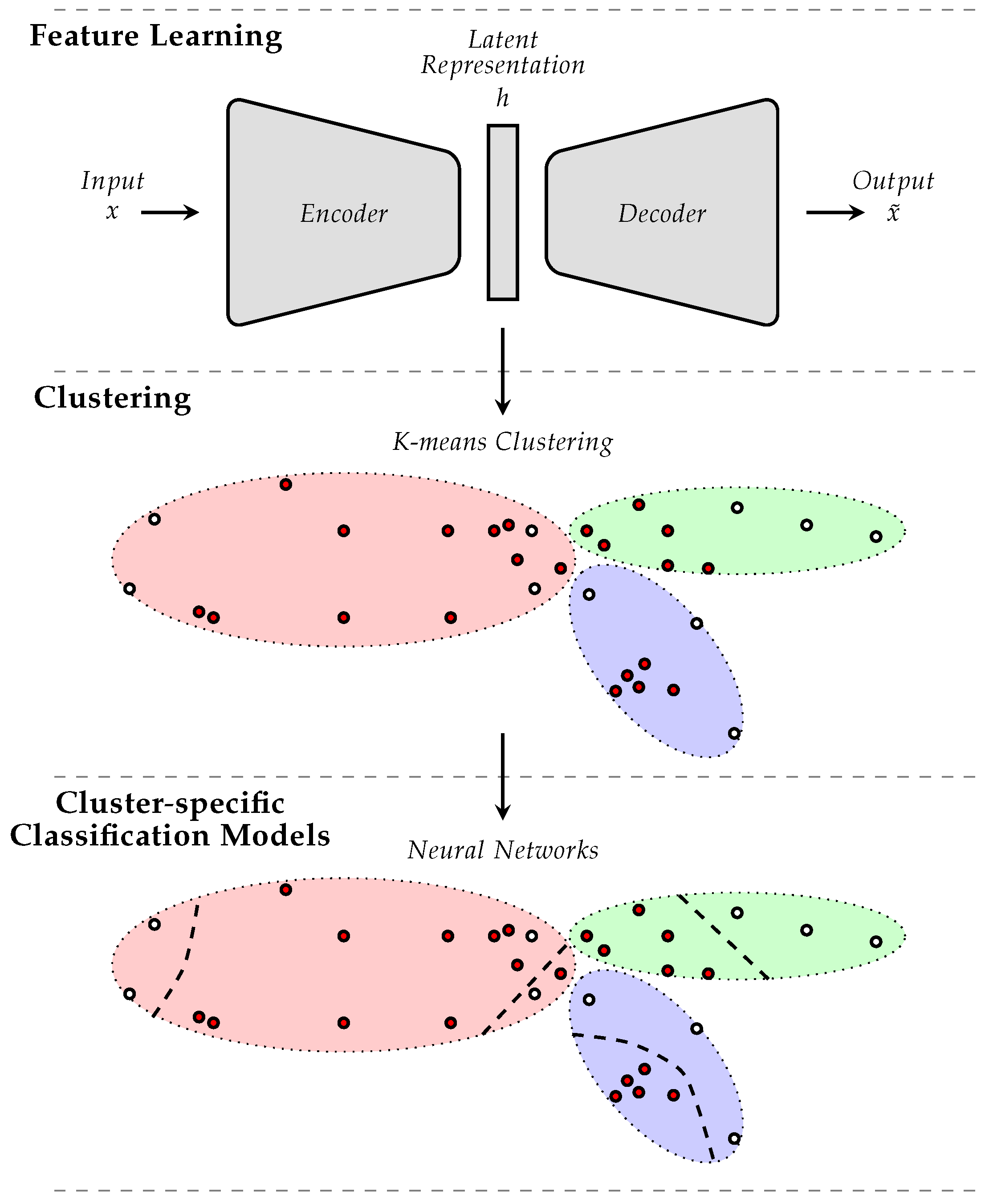
Figure 1. Proposed Approach. Feature Learning is performed to generate the latent space. Within the latent space, clustering is performed and corresponding samples’ weights are generated. Based on these weights, cluster-specific classification models are trained and subsequently used to perform the classification task.
Computers 14 00457 g001
Figure 2. Convolutional block (BN: batch normalization; ELU: exponential linear unit).
Computers 14 00457 g002
Figure 3. Classification results. Modality: EDA. Evaluation: leave one subject out (LOSO). Within each box plot, the red horizontal line corresponds to the median performance value, and the dark dot corresponds to the average performance value. (a) BioVid Part A ( T 0 vs. T 4 ). (b) BioVid Part B ( T 0 vs. T 4 ). (c) SenseEmotion ( T 0 vs. T 3 ).
Computers 14 00457 g003
Figure 4. Performance Comparison. Modality: EDA. Evaluation: Leave one subject out (LOSO). Within each box plot, the red horizontal line corresponds to the median performance value, and the dark dot corresponds to the average performance value. (a) BioVid Part A ( T 0 vs. T 4 ). (b) BioVid Part B ( T 0 vs. T 4 ). (c) SenseEmotion ( T 0 vs. T 3 ).
Computers 14 00457 g004
Table 1. DDCAE Architecture.
Encoder
BlockNo. Kernels/Units
2 × Convolutional Block 16
2 × Convolutional Block 32
2 × Convolutional Block 64
2 × Convolutional Block 128
Flatten
Decoder
BlockNo. Kernels/Units
Reshape
2 × Transposed Convolutional Block 128
2 × Transposed Convolutional Block 64
2 × Transposed Convolutional Block 32
2 × Transposed Convolutional Block 16
1 × Convolutional Layer 1
Table 2. Classification Results: average performance in % (standard deviation in %). Modality: EDA. Evaluation: leave one subject out (LOSO). The best performance is depicted for each dataset in bold, while the second best performance is underlined. An asterisk (*) depicts a significant performance improvement in comparison to the baseline. A dagger () indicates a significant performance improvement in comparison to the approach based on the DDCAE. The significance test was performed with a two-sided Wilcoxon signed-rank test with a significance level of 5 % .
DatasetBioVid Part A ( T 0 vs. T 4 )
ApproachBaselineCbSW (DDCAE)CbSW (IRM-DDCAE)
Accuracy 84.83 14.44 84.94 14.22 ̲ 85.32 13.71
F1-Score 83.65 16.90 83.81 16.59 ̲ 84.43 15.53
DatasetBioVid Part B ( T 0 vs. T 4 )
ApproachBaselineCbSW (DDCAE)CbSW (IRM-DDCAE)
Accuracy 78.40 15.88 78.69 15.68 ̲ 78.95 15.50
F1-Score 77.13 17.52 77.67 16.91 ̲ 78.07 16.58
DatasetSenseEmotion ( T 0 vs. T 3 )
ApproachBaselineCbSW (DDCAE)CbSW (IRM-DDCAE)
Accuracy 80.00 10.86 80.39 10.89 ̲ 81.50 10.19 * ,
F1-Score 79.29 11.91 79.77 11.80 ̲ 81.19 10.66 * ,
Table 3. Performance Comparison: average performance in % (standard deviation in %). Modality: EDA. Evaluation: leave one subject out (LOSO). The best performance is depicted for each dataset in bold.
DatasetBioVid Part A ( T 0 vs. T 4 )BioVid Part B ( T 0 vs. T 4 )SenseEmotion ( T 0 vs. T 3 )
ApproachPSOSWCbSWPSOSWCbSWPSOSWCbSW
Accuracy 85.03 13.84 85.32 13.71 78.60 15.69 78.95 15.50 81.24 10.19 81.50 10.19
F1-Score 84.25 15.37 84.43 15.53 77.70 16.18 78.07 16.58 80.88 10.73 81.19 10.66
Disclaimer/Publisher’s Note: The statements, opinions and data contained in all publications are solely those of the individual author(s) and contributor(s) and not of MDPI and/or the editor(s). MDPI and/or the editor(s) disclaim responsibility for any injury to people or property resulting from any ideas, methods, instructions or products referred to in the content.