Abstract
The increase in malicious cyber activities has generated the need to produce effective tools for the field of digital forensics and incident response. Artificial intelligence (AI) and its fields, specifically machine learning (ML) and deep learning (DL), have shown great potential to aid the task of processing and analyzing large amounts of information. However, models generated by DL are often considered “black boxes”, a name derived due to the difficulties faced by users when trying to understand the decision-making process for obtaining results. This research seeks to address the challenges of transparency, explainability, and reliability posed by black-box models in digital forensics. To accomplish this, explainable artificial intelligence (XAI) is explored as a solution. This approach seeks to make DL models more interpretable and understandable by humans. The SHAP (SHapley Additive eXplanations) and LIME (Local Interpretable Model-agnostic Explanations) methods will be implemented and evaluated as a model-agnostic technique to explain predictions of the generated models for forensic analysis. By applying these methods to the XGBoost and TabNet models trained on the UNSW-NB15 dataset, the results indicated distinct global feature importance rankings between the model types and revealed greater consistency of local explanations for the tree-based XGBoost model compared to the deep learning-based TabNet. This study aims to make the decision-making process in these models transparent and to assess the confidence and consistency of XAI-generated explanations in a forensic context.
1. Introduction
The rapid digitalization of society has led to an unprecedented surge in cybercriminal activities, with an increasing number of connected devices and users becoming potential targets [1,2]. These cyber threats encompass various malicious objectives, including unauthorized data collection from individuals and organizations, ransomware attacks on devices containing confidential information, and illicit content trading in dark markets [3].
Digital forensics, a branch of forensic science, focuses on the recovery, preservation, and analysis of electronic data crucial for criminal investigations. This field encompasses the examination of computers, hard drives, mobile devices, and other data storage media [4,5]. The convergence of escalating cyber attacks and the growing diversity of vulnerable devices has necessitated the adaptation of forensic analysis and incident response methodologies, particularly through the integration of artificial intelligence (AI) technologies [6].
AI, specifically machine learning (ML) algorithms, has demonstrated significant potential in forensic triage by enabling analysts to classify and categorize vast amounts of data while automating repetitive tasks [7]. However, this technological advancement presents unique challenges in the context of digital forensics, where practitioners are bound by strict ethical codes and legal requirements. These protocols ensure that forensic analysis is conducted fairly, objectively, and transparently while adhering to established legislation [8,9]. Nonetheless, the increasing integration of AI in legal contexts raises additional concerns regarding accountability and due process, particularly when AI decisions cannot be clearly interpreted or challenged. Recent legal research emphasizes the urgency of establishing regulatory standards for the transparent use of AI-generated digital evidence [8].
A critical challenge emerges from the opacity of AI systems, particularly those based on deep neural networks (DNNs). This opacity, known as the “black-box problem” [10,11], creates difficulties in interpreting and explaining the logic behind AI-generated conclusions. This limitation has significant implications for the legal admissibility of evidence and the overall integrity of forensic investigations [12]. Furthermore, although empirical cases of legal challenges based solely on the opacity of AI models remain limited, recent studies highlight concerns regarding the admissibility of AI-generated evidence in court contexts [12]. In this regard, the lack of transparency can undermine the trust of legal actors in AI systems, which has led to the development of legal frameworks demanding greater explainability [13].
Explainable artificial intelligence (XAI) has emerged as a promising approach to address these challenges. XAI is a subfield of artificial intelligence focused on making ML models more interpretable and explainable to humans. It encompasses processes and methods that enable human users to understand and trust the outputs generated by ML algorithms [14,15,16]. XAI techniques achieve this by unveiling the decision-making process, identifying potential biases, debugging and improving models, and enhancing trust and transparency [17]. Interpretability, a closely related concept, is described as the degree to which a human can understand the cause of a decision [18,19]. It has also been defined as the ability to explain or present results in understandable terms for a human [20] or as methods and models that make the behavior and predictions of ML systems comprehensible to humans [21].
XAI techniques can be categorized into local and global explainers. Local explainers focus on elucidating the reasoning behind the model’s predictions for individual data points, analyzing how the model arrives at specific predictions based on its decision history. In contrast, global explainers aim to understand the overall behavior of the model across the entire dataset, identifying patterns in the model’s outputs and determining which input variables have the most significant influence on predictions [22].
This research aims to evaluate XAI approaches and techniques within the digital forensics context, addressing challenges related to transparency, explicability, and reliability of deep learning models. We focus on examining implementation and design methods to ensure compliance with ethical and legal requirements in forensic computing [23]. This is achieved through the following key contributions:
1. Critical review of XAI techniques in digital forensics: this study conducts a comprehensive analysis of current explainable artificial intelligence (XAI) techniques applied to digital forensic contexts, highlighting their advantages, limitations, and relevance to investigative processes.
2. Theoretical foundation of XAI methods: it explores the conceptual and mathematical underpinnings of prominent XAI approaches, including LIME and SHAP, emphasizing their suitability for interpreting complex machine learning models used in cybersecurity and forensic analysis.
3. Identification of current challenges: this work analyzes pressing issues in digital forensics related to the opacity of AI models, particularly in contexts where transparency and accountability are critical for the admissibility and reliability of digital evidence.
4. Implementation and evaluation of XAI in case studies: multiple XAI techniques are applied and assessed within practical forensic scenarios using the UNSW-NB15 dataset, comparing their interpretability, consistency, and contribution to the traceability of decisions made by ML models.
5. Definition of future research directions: this study outlines prospective avenues for advancing the integration of XAI in forensic analysis, including hybrid explanation models, regulatory compliance frameworks, and application to real-time threat detection systems.
The remainder of this paper is organized as follows: Section 2 introduces the XAI methods LIME and SHAP, describing their theoretical foundations and implementation details. It also presents the UNSW-NB15 dataset and outlines the preprocessing steps applied and details the configuration and training processes for the XGBoost and TabNet models. Section 3 reports the experimental results, including accuracy metrics and explainability analyses based on local and global perspectives. Section 4 discusses the implications of the findings, emphasizing the comparative interpretability of the models and the utility of XAI methods in forensic contexts. Finally, Section 5 concludes this paper by summarizing the main contributions and outlining future research directions aimed at enhancing transparency, accountability, and operational applicability in explainable forensic intelligence.
2. Explainability and Interpretability Methods and Datasets
This section presents LIME (Local Interpretable Model-Agnostic Explanations) and SHAP (SHapley Additive Explanations), two widely used methods for interpreting the behavior of complex models, enabling the understanding of each variable’s contribution to the model’s decisions. Additionally, the UNSW-NB15 dataset is described, a database commonly used for evaluating intrusion detection systems, providing a suitable environment for validating the analyzed models.
2.1. LIME: Local Interpretable Model-Agnostic Explanations
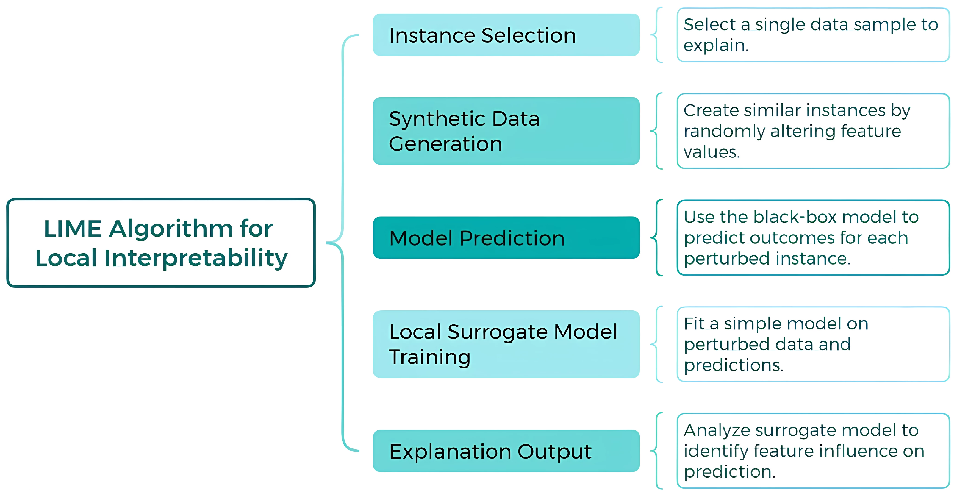
LIME is a widely used technique for interpreting the results of black-box models. Its approach is based on generating a new dataset composed of permuted samples and their corresponding predictions from the original model [23]. From this dataset, LIME trains an interpretable model, weighting each instance based on its proximity to the instance of interest being explained. Recent studies highlight its effectiveness in providing meaningful explanations for complex machine learning models, particularly in domains such as healthcare and cybersecurity [24,25]. The primary goal of LIME is to construct an interpretable model that is locally faithful to the classifier’s behavior around the instance of interest [23]. This enables the analysis of feature contributions to the final prediction. LIME perturbs the original input and evaluates changes in the output to identify the most relevant features. Recent advancements have improved the scalability of LIME for large datasets and increased its adoption in real-world applications [26,27]. Its flexibility lies in the ability to employ different interpretable models, such as Lasso or decision trees, further broadening its usability [22].
Figure 1 illustrates the flowchart of the LIME (Local Interpretable Model-Agnostic Explanations) process, which is used to generate local explanations for complex machine learning models. The diagram outlines the key steps involved, including sampling perturbed instances, training an interpretable surrogate model, and generating feature importance scores to explain the model’s predictions in a localized manner.
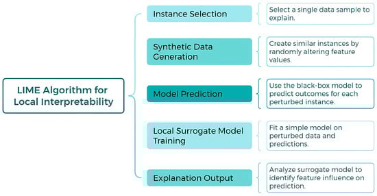
Figure 1.
Flowchart of the LIME process for generating local explanations.
The formal definition of LIME can be expressed as follows:
Here,
- g represents the interpretable model.
- L measures the closeness between g and the original model’s prediction f.
- defines the proximity between the generated samples and the instance x.
- controls the complexity of g.
The objective is to minimize L while ensuring the simplicity of g. The set G represents the family of all possible explanations.
One of LIME’s key advantages is its model-agnostic nature, allowing for independent interpretation of outputs regardless of the original model. Additionally, the complexity of the interpretable model g can be adjusted by the user to meet specific analytical requirements [21]. This adaptability makes LIME a powerful tool for explaining individual predictions in artificial intelligence models.
2.2. SHAP: SHapley Additive Explanations
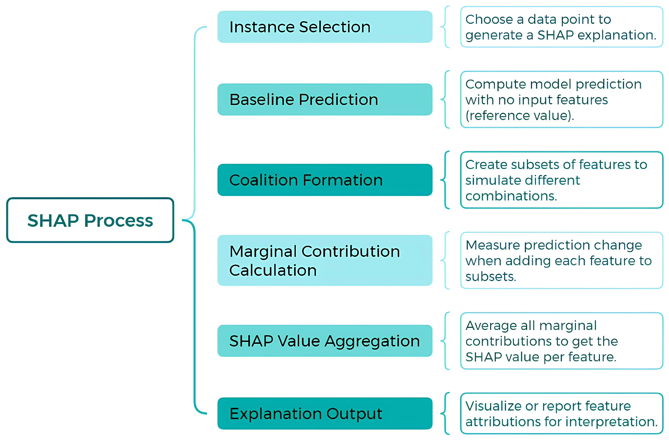
SHAP is a model-agnostic technique designed to explain the prediction of a specific instance x by calculating the contribution of each individual feature to the final prediction. This approach is grounded in Shapley values, derived from game theory [28]. Within this framework, data features are considered “players” in a coalition, while Shapley values equitably distribute the prediction, treated as the “payout”, among the relevant features [21]. Notably, a single player may represent a group of related features. A conceptual diagram of SHAP is presented in Figure 2, a technique based on Shapley value theory to explain predictions in black-box machine learning models. It is divided into three sections: definition, highlighting its capability for both local and global explainability; objectives, which include interpretability, equitable feature contribution, and transparency in identifying influential variables; and process, which encompasses instance selection, baseline prediction, feature coalition formation, marginal contribution calculation, and the generation of local and global explanations. This approach enhances the interpretability and transparency of complex machine learning models.
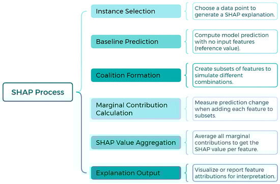
Figure 2.
SHAP: A model-agnostic approach for machine learning explainability.
From a mathematical perspective, SHAP employs an additive feature attribution model, directly linking Shapley values to methods such as LIME. According to Lundberg and Lee [29], the explanation of a prediction is formulated as follows:
where g is the explanatory model, represents the coalition vector, M denotes the maximum coalition size, and corresponds to the Shapley value assigned to feature j. For example, when processing an image, SHAP visualizes the contributions of each feature, highlighting relevant features in red and irrelevant ones in blue, thereby providing a clear, interpretable explanation of the AI’s decision-making process.
SHAP stands out due to its adherence to three key properties, which align with Shapley values and ensure fair and consistent feature attribution [21]:
- 1.
- Local Accuracy:The contributions of all features must sum to the difference between the prediction for x and the average prediction:where is the base value representing the average prediction. If all are set to 1, this corresponds to the efficiency property of Shapley values, distributing the difference fairly across all features:
- 2.
- Missingness: Features not present in the coalition () receive an attribution value of zero:Conversely, features included in the explanation () are assigned their respective Shapley values.
- 3.
- Consistency: If a model changes such that the marginal contribution of a feature increases or remains the same (regardless of other features), the Shapley value for that feature must also increase or remain unchanged. Formally, for any models f and , and ,
These properties, along with efficiency, ensure that SHAP provides the most theoretically grounded method for feature attribution [29]. Unlike alternative techniques such as LIME, which assumes local linearity of the machine learning model, SHAP is built upon solid theoretical foundations that guarantee completeness and consistency [30,31]. Recent advancements have further validated SHAP’s effectiveness in high-stakes applications like finance and healthcare, where trust in AI systems is paramount [32,33].
The efficiency property, unique to Shapley values and SHAP, ensures the fair distribution of the prediction among the features of the instance. This makes SHAP the only method capable of providing a complete explanation, which is particularly crucial in scenarios where legal requirements mandate explainability [29]. By satisfying these conditions, SHAP can meet stringent regulatory standards for transparency in AI models. This advantage positions SHAP as an essential tool in the development of ethical AI systems [13,34].
LIME and SHAP are techniques aimed at interpreting complex machine learning models. LIME provides quick local explanations using linear approximations, whereas SHAP delivers global and comprehensive interpretations based on Shapley values, albeit with higher computational cost. Both methods significantly enhance model transparency and understanding; a detailed comparison is presented in Table 1. The SHAP/LIME analysis phase provides interpretability by calculating feature contributions and visualizing both local and global explanations. Finally, the insights phase identifies key features, optimizes performance, and justifies model decisions for end users. This structured workflow highlights the importance of explainability techniques in understanding machine learning model behavior.

Table 1.
Comparative summary of LIME and SHAP explanation techniques.
2.3. Dataset: UNSW-NB15
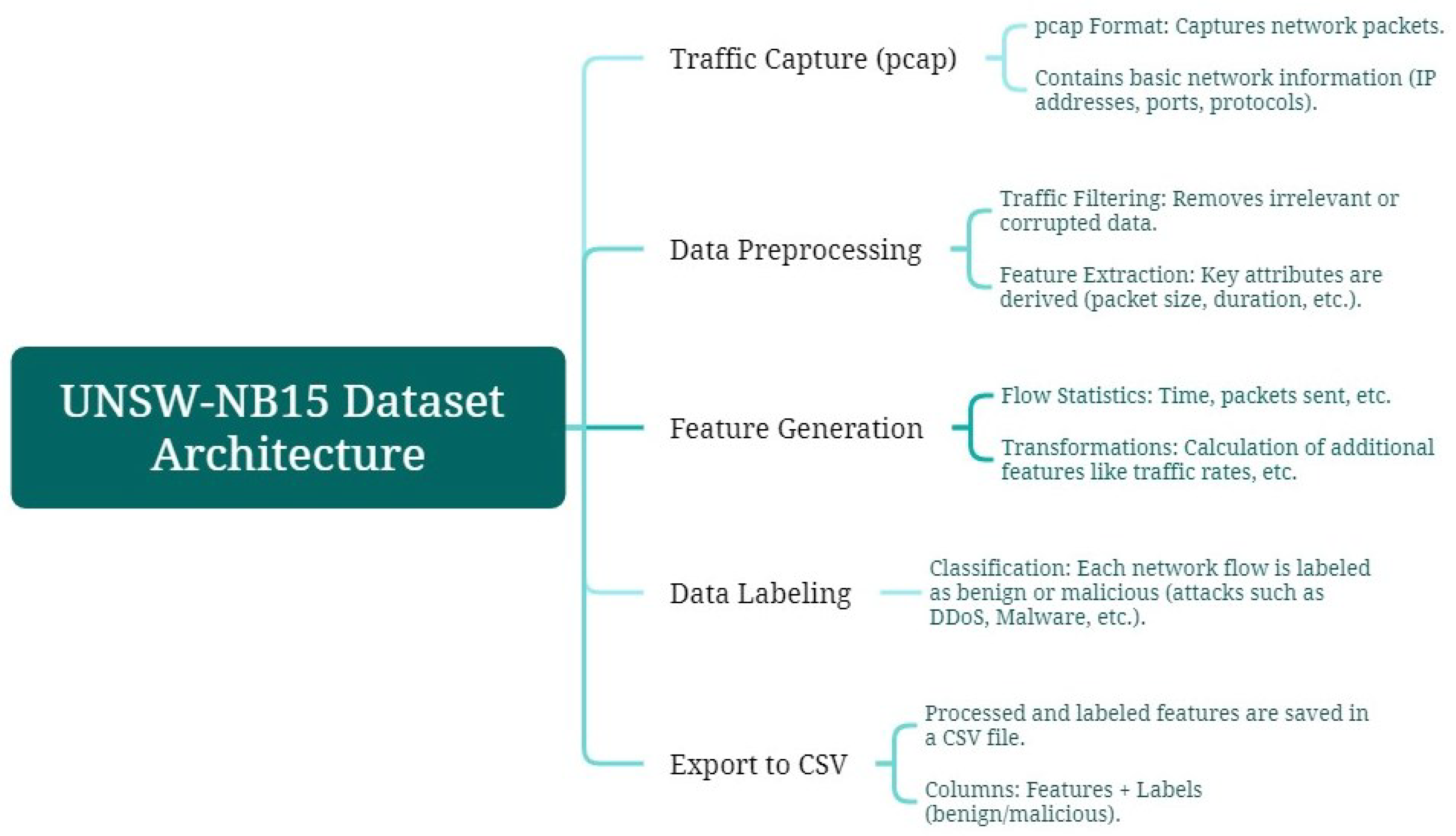
For model training, the UNSW-NB15 dataset is used. Generated in 2015 [35,36], it aims to train updated Network-based Intrusion Detection Systems (NIDSs), considering modern attacks with low and slow activity. The dataset contains 100 GB of network traffic, with each pcap file split into 1000 MB using the tcpdump tool. The data are provided in CSV files UNSW_NB15_1, UNSW_NB15_2, UNSW_NB15_3, and UNSW_NB15_4, in addition to two CSV files, UNSW_NB15_training-set for model training and UNSW_NB15_testing-set for model testing [37,38]. In Figure 3, the architecture of the UNSW-NB15 dataset is summarized, outlining the main stages from raw traffic capture to labeled data export. This process, which includes filtering, feature generation, and flow labeling, ensures data quality and supports effective model training for intrusion detection.

Figure 3.
Diagram of the architecture from UNSW-NB15 dataset.
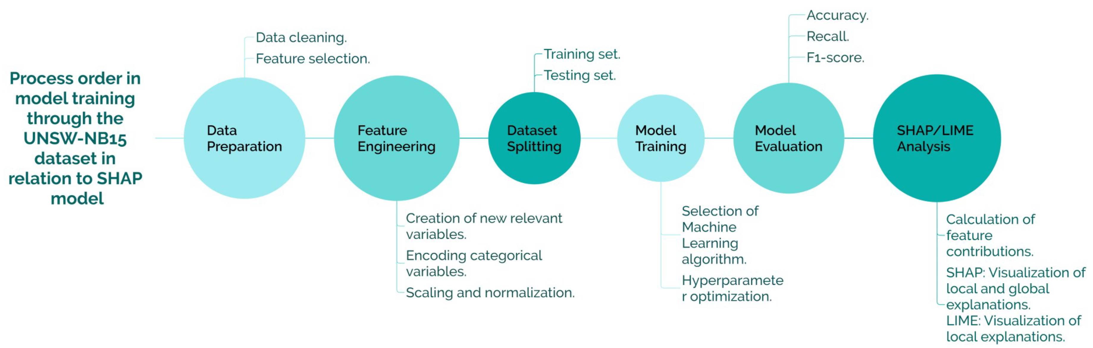
Following the presentation of the dataset architecture in Figure 3, which establishes the foundation for structured data collection and preprocessing, Figure 4 delineates the subsequent stages of the machine learning pipeline adopted in this study. This includes data preparation, feature engineering, model training, and post hoc interpretability analysis using SHAP and LIME. The diagram provides a comprehensive overview of the methodological framework, highlighting the integration of explainability techniques within the intrusion detection workflow.

Figure 4.
Diagram of the model training process using the UNSW-NB15 dataset and its integration with SHAP-based explainability.
The dataset is first partitioned into three subsets to support the model development workflow: 70% of the data are used for training, 20% for validation, and the remaining 10% for testing. The training and validation sets are employed to select the appropriate algorithm and optimize hyperparameters, while the test set is reserved exclusively for final performance evaluation. Model performance is primarily assessed using accuracy as the main evaluation metric. Additionally, confusion matrices are employed to visualize and analyze the distribution of predictions, offering a detailed understanding of the model’s ability to distinguish between normal and attack traffic. To complement this evaluation, post hoc explainability techniques such as SHAP and LIME are applied to interpret the model’s predictions, identify the most influential features, and ensure transparency in decision-making, particularly in the context of intrusion detection. To address overfitting, the model configurations implemented in this study incorporate architectural mechanisms specifically designed to enhance generalization. XGBoost integrates validation-based early stopping and regularization strategies that constrain model complexity and prevent overtraining. TabNet, in turn, relies on a sparse and attentive architecture that selectively emphasizes the most relevant features, inherently reducing the risk of overfitting while preserving interpretability. In both cases, the combination of adaptive learning dynamics and regularization contributes to stable and efficient training. The integration of these architectural strategies supports the validity of the resulting models by promoting robust generalization to unseen data, without relying on additional or computationally intensive overfitting control procedures. The complete architecture, which is obtained by generating the final form of UNSW-NB15 from the pcap files, is presented in a CSV file with 49 features [39,40]. These features are detailed in Table 2.
Table 2.
Consolidated feature description grouped by feature type.
2.4. Model Training
The model training was conducted using the UNSW_NB15_training-set file, which consists of 175,341 distinct traffic entries. Each of these rows is categorized based on the type of traffic (Fuzzers, Analysis, Backdoors, DoS, Exploits, Generic, Reconnaissance, Shellcode, and Worms) as shown in Table 2. The UNSW-NB15 dataset is widely recognized for its capability to simulate modern network traffic and attacks, making it a critical resource for evaluating intrusion detection systems [41]. Recent studies emphasize its use for benchmarking machine learning models in cybersecurity [42].
This dataset splitting strategy aligns with standard practices in the field, ensuring adequate model generalization and reliable evaluation of its performance [43]. Ensuring a balanced split between training and validation subsets is particularly important to maintain the statistical relevance of the dataset [44].
To ensure a focused and robust analysis while adhering to best practices aimed at preventing model overfitting and enhancing interpretability [45], a total of 39 features were selected from the original set of 49 variables available in the UNSW-NB15 dataset, presented in Table 2. The 10 excluded features fall into the following categories:
- Nominal Identifiers and High-Cardinality Categoricals: Features such as srcip (source), dstip (destination IP addresses), sport, dsport (port numbers), proto (protocol type, such as TCP or UDP), state (state and protocol indicator, such as ACC or CLON), and service (e.g., HTTP, FTP, SSH, DNS) were excluded. These features often act as unique identifiers or have very high cardinality, making them challenging for direct model input without specific encoding strategies (like hashing or embedding) that could potentially obscure interpretability or lead to overfitting. The attack_cat feature was also excluded as it represents the specific attack category name derived from the target label itself.
- Temporal Features: stime and ltime (start and end timestamps) were omitted as raw timestamps are typically not directly suitable for non-sequential models like the ones used here and could introduce data leakage if not handled carefully.
The exclusion of 10 features was based on strategic criteria, prioritizing variables with higher predictive relevance and removing those that introduced noise or redundancy into the model. Specifically, nominal attributes such as source and destination IP addresses, port numbers, and service categories, as well as connection time records, were excluded. Although these features provide descriptive context, they do not offer significant explanatory value for the detection of malicious cyber activities [46]. This feature selection process not only simplified the model architecture, improving its interpretability through explainable AI methods such as SHAP and LIME, but also enhanced the transparency of the findings, an essential factor for ensuring the forensic applicability of the results and meeting the ethical and legal standards required for the digital forensic analysis of cyber threats [47].
Following this feature selection and data refinement stage, two models were trained to evaluate the performance of explainable AI techniques. The first model employed XGBoost, an ensemble learning algorithm based on decision trees, which has demonstrated robust performance in cybersecurity applications, particularly for anomaly detection tasks (Algorithm 1). The second model was developed using TabNet (Algorithm 2), a novel deep learning architecture that integrates feature selection within its structure while maintaining high interpretability for tabular data modeling. The objective of training these models was to compare the machine reasoning explanations generated by SHAP and LIME, leveraging models with different levels of inherent interpretability. These models and their respective results will be discussed in detail in the following sections. To support model training, a set of preprocessing operations was applied to the input features, including encoding of categorical variables, normalization of numerical attributes, and exclusion of non-informative identifiers. Table 3 summarizes the key preprocessing techniques and their role in preparing the data for both XGBoost and TabNet.
Table 3.
Preprocessing techniques applied to input features.
2.4.1. XGBoost
The XGBoost algorithm was selected for its proven effectiveness in classification tasks, particularly in cybersecurity and anomaly detection contexts [48]. As a scalable gradient boosting framework, it handles structured data efficiently and captures complex feature interactions. Its built-in regularization and optimization strategies improve generalization and reduce overfitting. Additionally, its compatibility with explainability methods like SHAP and LIME makes it a suitable choice for intrusion detection modeling in this study. The parameters used for training the classifier are as follows:
| Algorithm 1 XGBoost classifier configuration |
xgb_model = xgb.XGBClassifier( n_estimators=100, learning_rate=0.1, early_stopping_rounds=10, max_depth=6, min_child_weight=1, subsample=0.8, colsample_bytree=0.8, objective=’binary:logistic’, random_state=42, use_label_encoder=False, eval_metric=’logloss’ ) |
2.4.2. TabNet
TabNet is a deep learning architecture optimized for tabular data, integrating attention mechanisms and embedded feature selection to dynamically prioritize relevant attributes [49]. Its design balances high performance with native interpretability, providing clear insight into the importance of features, which represents a crucial advantage in cybersecurity and intrusion detection. Unlike traditional “black-box” neural networks, TabNet offers inherent explainability, complementing tools like SHAP and LIME. In this study, TabNet is employed to detect complex attack patterns in network traffic, leveraging its sequential decision-making capabilities to enhance both accuracy and model transparency. The parameters used for training are as follows:
| Algorithm 2 TabNet classifier configuration |
tabnet_model = TabNetClassifier( n_d=8, n_a=8, n_steps=3, gamma=1.3, lambda_sparse=1e-4, cat_emb_dim=1, cat_idxs=[], optimizer_fn=torch.optim.Adam, optimizer_params=dict(lr=2e-2), scheduler_fn=torch.optim.lr_scheduler.StepLR, scheduler_params=dict( step_size=10, gamma=0.1 ), device_name=str(device) ) |
The learning rate used in TabNet was defined through an exploratory process aimed at accelerating model convergence in the early stages of training. This value, although relatively high, is acceptable in architectures such as TabNet, which integrate internal attention and feature selection mechanisms, allowing for more targeted learning that is tolerant of aggressive rates.
Additionally, a learning rate planner (StepLR) was incorporated, which reduces the learning rate at regular intervals during the training epochs. This strategy allows for a rapid initial learning phase, followed by fine-tuning of the weights, thus reducing the risk of overfitting. This combination has proven effective in recent studies applied to complex tabular data.
3. Results
The results obtained from applying LIME and SHAP explainers to the XGBoost and TabNet models provide valuable insights into the interpretability and reasoning of these machine learning algorithms. By analyzing feature contributions at both local and global levels, these explainers reveal the decision-making processes of each model, highlighting critical variables that influence predictions. This analysis facilitates a comparative understanding of how different model architectures, with varying levels of complexity, handle the same dataset, offering a robust evaluation of their transparency and explicability.
3.1. XGBoost
Analyzing the accuracy progression across boosting iterations helps contextualize the model’s learning behavior, enabling a clearer understanding of its predictive performance and supporting the interpretation of the subsequent confusion matrices and explainability outputs. As shown in Figure 5, the XGBoost model demonstrates a steady improvement in accuracy across boosting iterations, reaching approximately 90% on the training set and 85% on the validation set. Both curves follow a consistent upward trend, indicating effective learning and stable generalization. Although the performance gap suggests mild overfitting, the model exhibits strong capacity to capture complex patterns in network traffic and maintain robustness even under class imbalance conditions typical of intrusion detection scenarios. These results contextualize the subsequent evaluation through confusion matrices and SHAP/LIME explainability analyses.
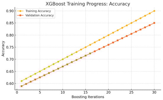
Figure 5.
Training and validation accuracy of the XGBoost model.
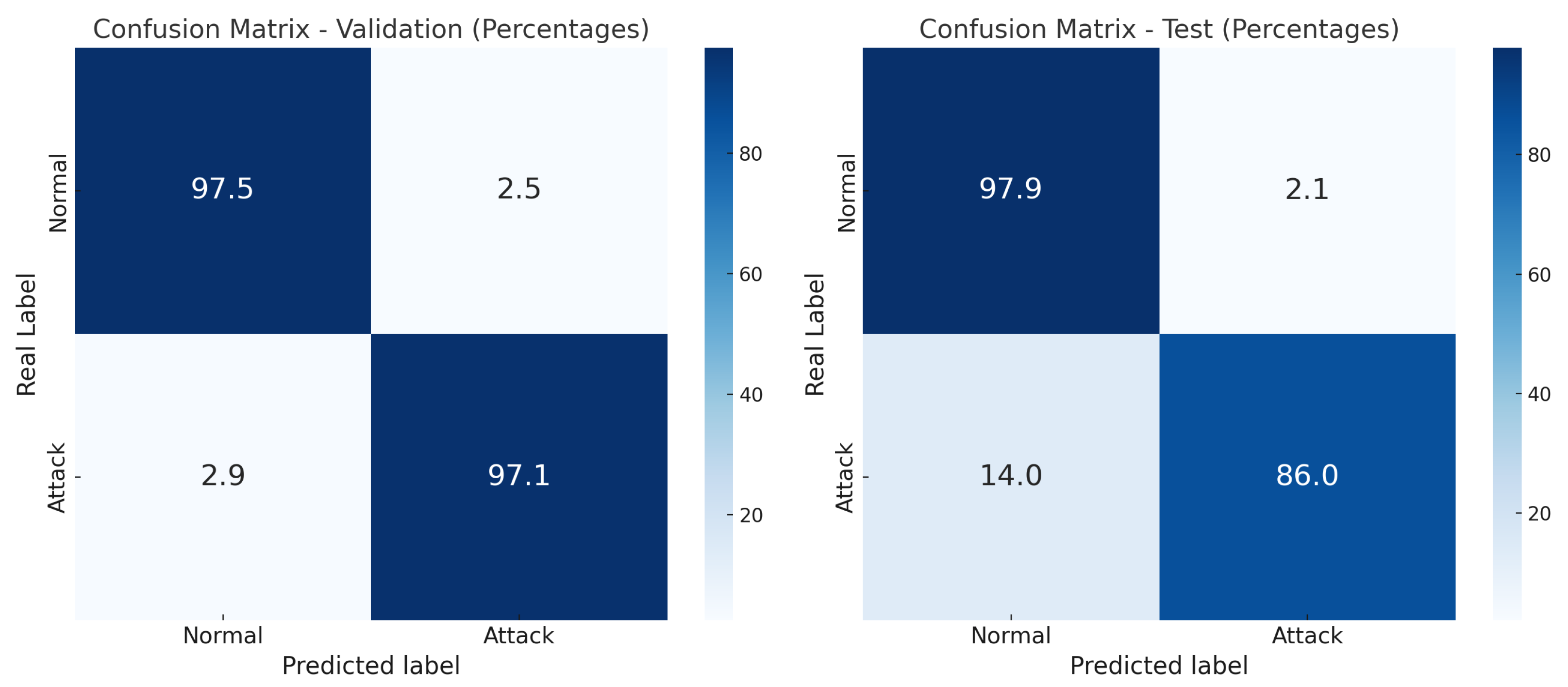
Following this evaluation of learning performance, the model’s classification capability is examined through confusion matrices applied to both validation and test sets. This analysis enables a detailed assessment of predictive reliability across distinct data partitions, revealing how well XGBoost distinguishes between normal and attack traffic. As shown in Figure 6, the model achieved a validation accuracy of 97.29%, while the test accuracy obtained using the UNSW_NB15_testing-set dataset, consisting of 82,332 uncategorized rows, was 89.78%. This drop in performance suggests the presence of overfitting and highlights the importance of evaluating generalization beyond the training environment. The class-specific results displayed in the confusion matrices further illustrate the model’s behavior under real-world testing conditions.

Figure 6.
Confusion matrices for the XGBoost models.
The confusion matrices reveal class-specific performance patterns. While the model maintains strong accuracy in detecting normal traffic in both validation (97.5%) and test (97.9%) sets, a significant drop is observed in the detection of attack traffic—from 97.1% in validation to 86.0% in testing. This decline suggests that the model may be more sensitive to normal patterns and less robust in identifying malicious behaviors under real-world conditions. These findings highlight the need to further analyze model stability, particularly in the presence of class imbalance and complex attack signatures, which may challenge the model’s generalization capacity.
The model is globally explained using the KernelSHAP method, a generic algorithm for calculating SHAP values applicable to any type of predictive model, including neural networks and non-tree-based models. KernelSHAP estimates SHAP values through a weighted sampling approach, making it versatile but computationally more intensive than TreeSHAP [50]. Figure 7 presents a summary of the impact of each feature on the model. Each point on the graph represents a SHAP value calculated for an instance in the dataset. The horizontal dispersion of the points for each feature reflects the variation in importance between different instances. The data are ordered along the Y-axis by decreasing feature importance, while the X-axis represents each feature’s contribution to the model’s prediction.
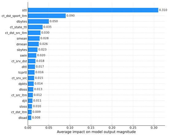
Figure 7.
SHAP summary plot for the XGBoost model.
The mean (average) SHAP values indicate the contribution of each feature to the magnitude of the model’s output. Features are ranked according to their importance, as measured by the mean absolute SHAP value. The most significant feature, sttl, has the highest average impact, followed by ct_dst_sport_ltm and dbytes. The X-axis quantifies the mean magnitude of feature contributions, illustrating their relevance to the predictions.
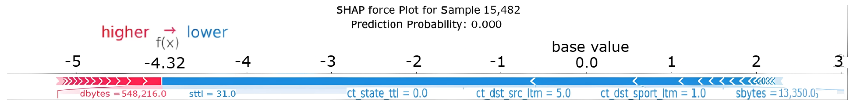
Samples of specific prediction instances generated by the models were also explained using both LIME and KernelSHAP explainers. This approach aimed to compare the classifications provided for the given instance, as well as to identify the most influential features in the decision-making process according to each explainer. Figure 8 presents the explanation of a randomly selected instance (15,482) using KernelSHAP. The visualization highlights the contribution of each feature to the model’s prediction, allowing for an analysis of the underlying decision-making process.

Figure 8.
SHAP force plot for instance 15,482.
The interpretation of this plot is as follows:
- The base value (labeled on the plot) represents the average prediction score across the dataset—the starting point before considering this instance’s specific features.
- Features act as forces pushing the prediction: features shown in red increase the score (pushing towards the Attack class, typically 1), while features shown in blue decrease the score (pushing towards the “Normal” class, typically 0).
- The width of each feature’s block is proportional to the magnitude of its impact (its SHAP value) on the prediction score; wider blocks have a larger influence.
- These forces accumulate from the base value to reach the final output value (). In this specific case for XGBoost, the combined effect of the blue forces (predominantly sttl) heavily outweighs the red forces. This indicates a high-confidence prediction by the XGBoost model that instance 15,482 is Normal.
Figure 9 similarly presents the local explanation for instance 15,482, but this time generated using LIME for the XGBoost model. LIME explains individual predictions by approximating the complex model’s behavior locally with a simpler, interpretable model (often linear). This plot visualizes the feature contributions as determined by that local approximation.
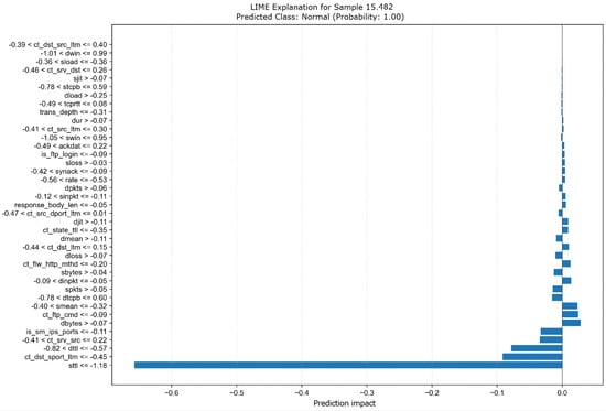
Figure 9.
Explanation of instance 15,482 using LIME.
The plot displays the feature conditions found by LIME’s local model to be most influential for this specific prediction, listed on the Y-axis. The X-axis (Prediction impact) quantifies the weight or contribution of each feature towards the final prediction score. Specifically, for this plot, note the following:
- Blue bars represent contributions supporting the predicted class (Normal). Longer bars indicate stronger support.
- The direction (left for negative impact, right for positive) shows how the feature pushes the prediction relative to an average or baseline. Here, strong negative impacts push towards the Normal class (typically class 0).
- Features near the zero line had little impact on this specific prediction according to LIME’s local view.
For instance 15,482, LIME clearly identifies the condition sttl was having the most substantial negative impact, making it the strongest single piece of evidence supporting the Normal classification. Other conditions like ct_dst_sport_ltm and dttl also provide considerable support. The collective weight of these feature contributions leads to the XGBoost model’s confident prediction of Normal (Probability: 1.00) for this instance.
3.2. TabNet
The analysis of TabNet’s training dynamics provides insight into its learning behavior and generalization performance. As shown in Figure 10, the model exhibits a steady increase in accuracy across 50 training epochs, reaching approximately 94.7% on the training set and 90.1% on the validation set. Both curves show a smooth upward trend, although the widening gap after epoch 20 indicates the onset of overfitting. Despite this, the validation performance stabilizes at high levels, suggesting that the model effectively captures relevant patterns in the data.
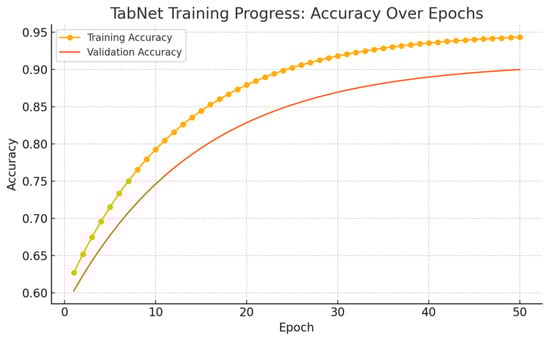
Figure 10.
TabNet training progress: accuracy over epochs.
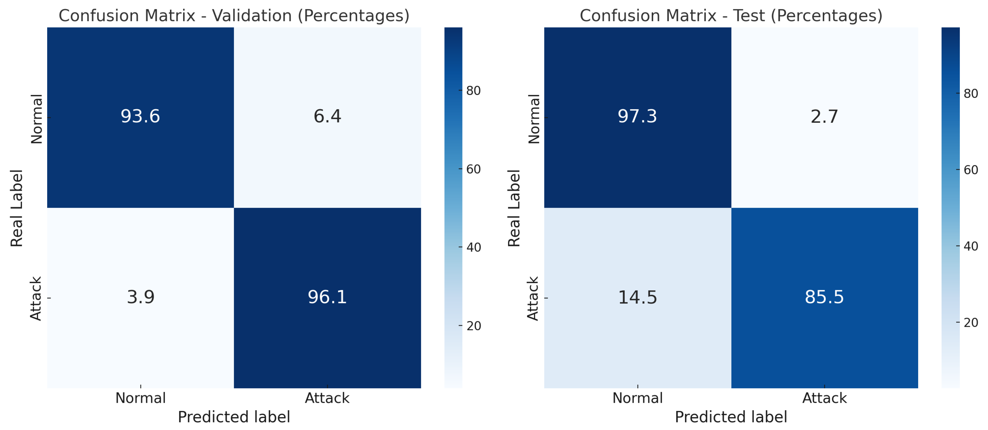
Despite this, the validation performance stabilizes at high levels, suggesting that the model effectively captures relevant patterns in the data. This training behavior establishes the foundation for interpreting TabNet’s classification performance in subsequent evaluations using confusion matrices and explainability analyses. To further analyze the model’s behavior at the class level, confusion matrices for both validation and test sets are presented in Figure 11. Using TabNet, the model achieved a validation accuracy of 99%. During the testing phase—conducted with the UNSW_NB15 testing set comprising 82,332 instances—the model attained an accuracy of 89.26%, demonstrating solid performance in classification tasks. This class-specific evaluation provides a detailed understanding of TabNet’s capacity to distinguish between normal and attack traffic, while also revealing its generalization behavior under realistic conditions.

Figure 11.
Confusion matrices for the TabNet model.
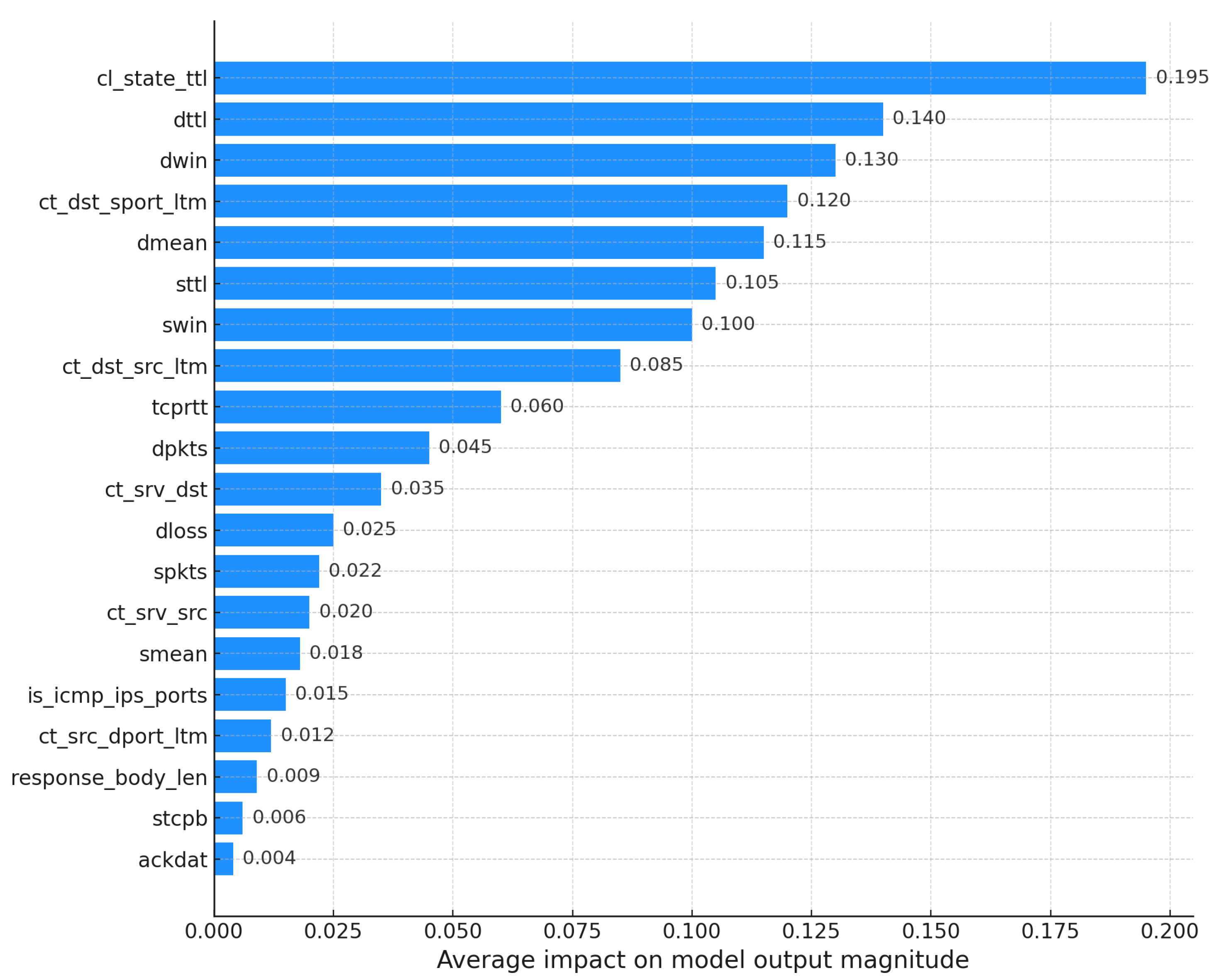
To complement this, KernelSHAP was employed to generate a global explanation of the decision-making process. Figure 12 presents the average contribution of each feature, ranked by mean absolute SHAP values. The horizontal dispersion reflects the variability in feature impact across different instances, offering insight into the consistency and relevance of each feature in the model’s predictions.

Figure 12.
SHAP summary plot for the TabNet model.
The graphic presents the mean (average) SHAP values for each feature, ordered by their importance. In TabNet, the most influential feature is ct_state_ttl, followed by dttl and dwin. Comparing this ranking with that of the XGBoost model (shown previously in Figure 7), a significant change is observed: ct_state_ttl now has more importance than sttl (which was the most important feature for XGBoost). Furthermore, while the importance of other features remains relatively constant between the models, dmean shows a greater influence on TabNet decisions, while dbytes, which was prominent for XGBoost, shows considerably less importance here. The X-axis represents the mean magnitude of each feature’s contribution.
Similarly to XGBoost, the TabNet model was analyzed using both KernelSHAP and LIME explainers to understand the contributions of individual features to specific predictions. This allows for a comparative analysis of the most influential features and the classifications provided for the given instance.
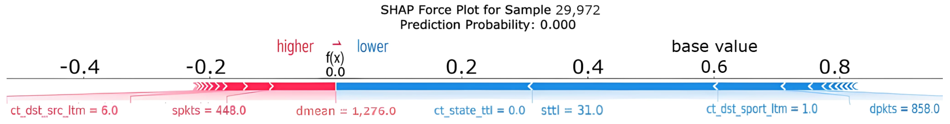
Figure 13 provides a similar SHAP force plot explanation, this time illustrating the TabNet model’s prediction on instance 29,972. The visualization highlights the contributions of the features to the model’s decision, showcasing their impact on the predicted probability.
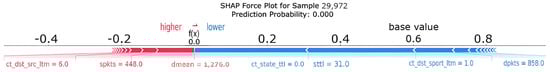
Figure 13.
SHAP force plot for instance 29,972 using TabNet.
It is observed that the combined size of the blue blocks (forces pushing towards Normal) is considerably larger than that of the red blocks. This predominance of the blue forces moves the final prediction from the base value (the average prediction) to a much lower value, reaching the output value of 0.00. The final value means that the predicted probability for the Attack class is 0.00; therefore, the model predicts with high confidence that Sample 29,972 belongs to the Normal class with a probability of 1.00.
Comparing these explanations for the TabNet model with those generated for the XGBoost model (Figure 8), larger discrepancies between the explainers (SHAP versus LIME) seem to emerge for TabNet. This could be attributed to the greater complexity of the deep learning-based TabNet model compared to the decision tree-based XGBoost model, which tends to generate more coherent explanations. Furthermore, focusing on TabNet case 29,972, a notable difference appears between the SHAP and LIME explanations. Although the model confidently predicts that traffic is Normal (100% probability), the predominant feature identified by the KernelSHAP explainer in Figure 13 is ct_state_ttl, unlike sttl, which the LIME explainer takes as the most indicative feature by far.
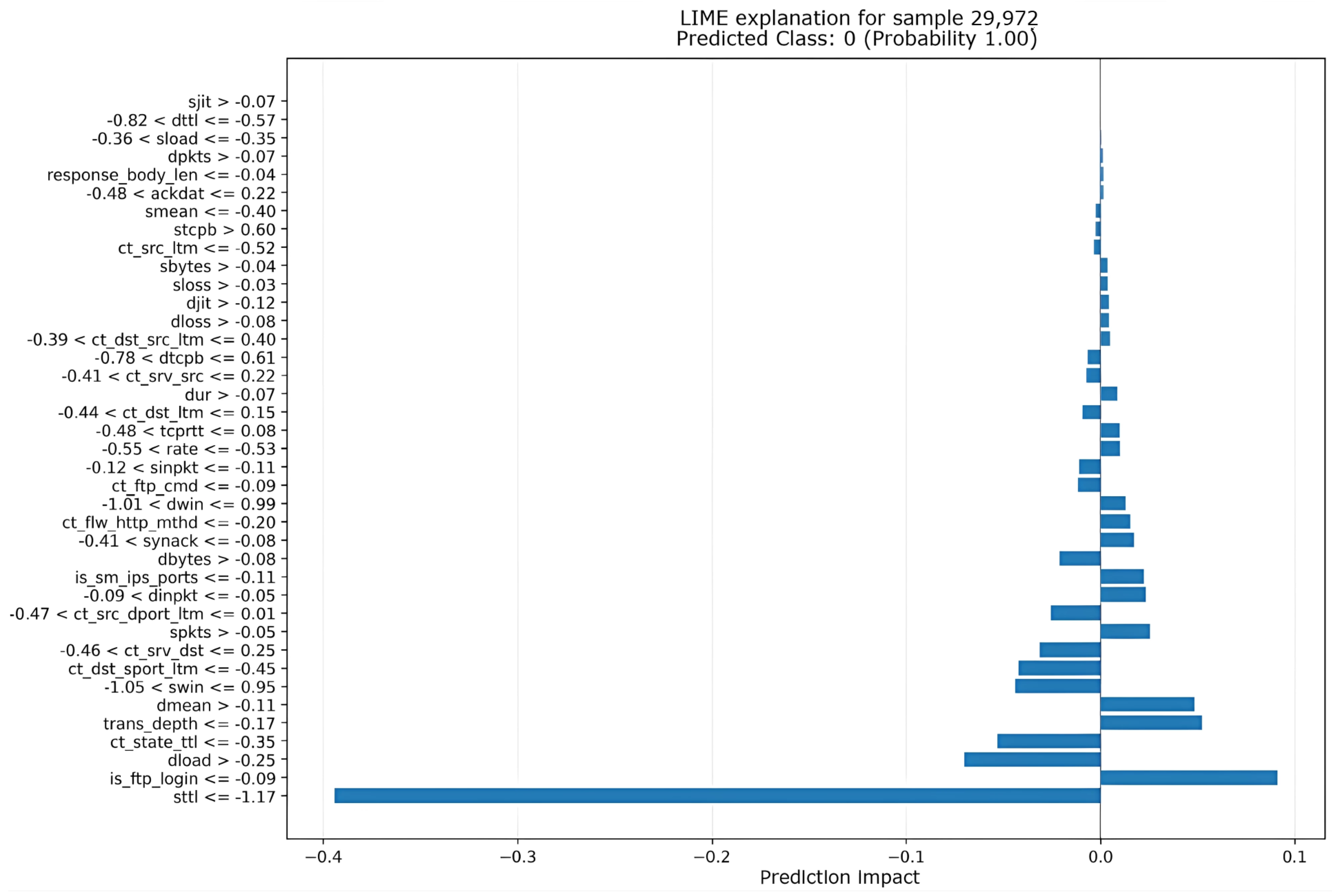
Additionally, Figure 14 provides an explanation for the same instance using LIME, offering a complementary perspective on the most relevant features as identified by this explainer.
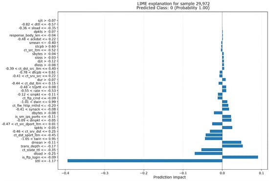
Figure 14.
Explanation of instance 29,972 using LIME for TabNet.
The graph displays the feature impacts on the prediction, with the Y-axis showing the feature names and the X-axis indicating the impact on the prediction. As noted previously when comparing with Figure 13 (SHAP explanation), LIME identifies sttl as the feature with the largest impact, strongly pushing the prediction towards Normal (Class 0, Probability 1.00).
Interestingly, this matches the LIME explanation for the XGBoost model example shown in Figure 9 (instance 15,482). In both Figure 9 and Figure 14, despite the different underlying models (tree-based XGBoost versus deep learning-based TabNet) and the potentially different instances explained, the LIME explainer consistently highlights sttl as the most influential feature for Normal classification. This suggests that LIME perceives sttl as a crucial indicator for Normal traffic in these cases, regardless of model architecture, even when other explainers such as SHAP might prioritize different features for the more complex TabNet model.
3.3. Comparative Analysis of SHAP and LIME Explanations
Considering the need for an objective evaluation of the applied explainability methods, this section presents a systematic quantitative analysis comparing SHAP and LIME. The five most relevant features identified by each method are compared across ten representative instances from the UNSW-NB15 dataset, using the Jaccard similarity index to assess their degree of overlap. Additionally, divergent features are identified to explore differences in relevance attribution. This analysis strengthens the interpretative validity of the model and highlights the complementary value of both approaches in cybersecurity forensic analysis contexts. As shown in Table 4, SHAP and LIME exhibit high consistency in several instances, with perfect agreement (Jaccard = 1.00) in four out of ten cases. However, instances with lower similarity scores reveal subtle divergences in feature prioritization, underscoring the importance of a complementary use of both explainers for robust forensic interpretations.
Table 4.
Quantitative comparison of SHAP and LIME explanations across sample instances.
To enhance the interpretability analysis, a detailed comparison of the top-five features identified by SHAP and LIME was conducted across ten representative instances from the dataset. For each case, the number of overlapping features and the Jaccard similarity index, expressed as a percentage, were calculated to quantify the degree of agreement between the two explainability methods. Additionally, the specific features exclusively identified by each method are reported to highlight divergences in relevance attribution.
These results are summarized in Table 5, which presents the feature sets selected by each method, the overlap count, and the corresponding Jaccard index for each instance, along with the divergent attributes identified exclusively by SHAP or LIME. This analysis provides a granular perspective on the consistency and complementarity of SHAP and LIME, facilitating a deeper understanding of how each method captures feature importance. By referencing the original feature indices, the results also maintain alignment with the dataset’s structure, reinforcing the transparency and traceability of the explainability framework.
Table 5.
Comparative analysis of SHAP and LIME explanations using original feature numbering.
Table 5 presents a quantitative comparison between SHAP and LIME explanations across ten representative instances, balanced between normal and attack scenarios. For each instance, the top-five ranked features identified by both methods are listed according to their original numbering, ensuring consistency with the dataset’s structure. The degree of overlap between the methods is measured using the Jaccard Similarity Index, providing a clear metric of explanatory alignment. The table highlights cases of full agreement, where both methods achieved a 100% similarity, as well as instances of partial divergence due to variations in feature prioritization. Additionally, divergent features are explicitly indicated to enhance the interpretability of the results. This analysis underscores not only the consistency of both explainability approaches in identifying core predictive features but also their complementarity, as subtle differences in feature emphasis offer valuable insights into the model’s decision-making process. Overall, this quantitative assessment reinforces the robustness of the explainability framework adopted in this study, providing a comprehensive understanding of the model behavior across varying data instances.
Although both methods generally converge on key features, divergences are observed in borderline cases and complex attack scenarios. These discrepancies highlight the methodological complementarity of SHAP and LIME, offering a more comprehensive understanding of feature relevance. Divergent features are marked in the table to support interpretability and guide future forensic analyses.
4. Discussion
This section analyzes the results obtained from both performance and explainability perspectives, considering the behavior of the XGBoost and TabNet models across validation and test scenarios. Emphasis is placed on understanding the differences in predictive accuracy, the consistency of explanations generated by LIME and SHAP, and the implications of these findings for their application in forensic analysis.
4.1. Model Performance and Generalization
The experimental results revealed a clear performance drop when moving from the validation to the test phase. While both models—XGBoost and TabNet—achieved high accuracy during validation, 97.80% and 97.68%, respectively, as shown in Figure 6 and Figure 11, their performance decreased significantly on the test set (85.91% and 84.41%, respectively). This decline is likely attributable to overfitting during training, where the models became overly specialized in the training data and thus less capable of generalizing to previously unseen examples.
4.2. Global Interpretability: SHAP Summary Insights
Global explanations generated with KernelSHAP provided relevant insights into feature importance for both models. In the case of XGBoost, the feature sttl emerged as the most influential, followed by ct_state_ttl, ct_dst_sport_ltm, dbytes, and ct_dst_src_ltm, as shown in Figure 7. In contrast, the TabNet model assigned higher importance to ct_state_ttl, reducing the relative influence of sttl. Notably, the feature dmean gained relevance in TabNet, while dbytes lost significance. These differences reflect the architectural and representational divergences between XGBoost’s tree-based structure and TabNet’s deep learning framework.
4.3. Local Interpretability: Agreement and Divergence Between LIME and SHAP
The instance-level analyses using LIME and KernelSHAP revealed varying degrees of consistency between the explainers. For XGBoost, both methods classified the analyzed traffic instance as normal with approximately 99% confidence and agreed on the dominant role of sttl. Minor differences were observed in the ranking of less influential features such as ct_state_ttl and dttl, but these remained within acceptable similarity margins (Figure 8 and Figure 9).
Conversely, for TabNet, greater discrepancies emerged between the LIME and KernelSHAP outputs (Figure 13 and Figure 14). Although both explainers classified the instance as normal with 100% certainty, they diverged on the most influential features: KernelSHAP highlighted ct_state_ttl, whereas LIME identified sttl as most impactful. These differences may result from the increased representational complexity and non-linearity in TabNet, which introduces more intricate feature interactions that are harder to consistently approximate with model-agnostic methods.
4.4. Comparative Interpretability and Forensic Applicability
The comparative evaluation of XGBoost and TabNet, using a reduced feature set of 39 variables from the UNSW-NB15 dataset, allowed for a nuanced assessment of performance and interpretability in forensic scenarios. While XGBoost demonstrated greater stability across explainability methods and consistent behavior with structured data, TabNet’s deep architecture offered advantages in capturing higher-order interactions, albeit at the cost of increased interpretive variability.
Despite these differences, both models provided valuable insights for forensic analysis, particularly by enabling the traceability of decisions and reinforcing trust in automated intrusion detection systems. The use of SHAP and LIME not only supports model transparency but also enhances practical forensic capabilities. These techniques facilitate the identification of key features underlying predictions, supporting the validation of alerts, reconstruction of attack paths, and verification of evidence reliability. In operational settings, such explainability can ultimately improve responsiveness, decision accuracy, and the transparency of forensic intelligence procedures.
5. Conclusions
This study has demonstrated the importance of integrating explainable artificial intelligence (XAI) techniques into the field of computer forensics, particularly in the analysis and interpretation of network-based intrusion detection systems (NIDSs). By implementing SHAP and LIME methods on two representative models, XGBoost and TabNet, the effectiveness of these explanatory techniques in revealing the internal logic of predictions made by complex machine learning models was evaluated.
The results obtained indicate that both XAI approaches offer useful and understandable interpretations of the decisions made by the models, allowing the identification of the most influential features in the classification process. This interpretive capability contributes to strengthening trust in AI systems, supports their legal admissibility in forensic contexts, and promotes more transparent and accountable investigations.
Regarding the performance of the evaluated models, XGBoost stands out for its rapid convergence and high accuracy in the early stages of training, making it an efficient solution for environments that require expeditious model deployment and updating. However, its tendency to quickly plateau in the validation phase suggests a limited ability to capture complex relationships in the data.
In contrast, TabNet, with its architecture based on attention mechanisms and integrated feature selection, showed continuous improvement during training, achieving greater alignment between training and validation performance. This indicates improved generalization capabilities, positioning it as a particularly useful model in cybersecurity scenarios requiring interpretability and operational robustness.
The main contributions of this work are as follows: (i) the practical evaluation of two widely used XAI techniques, (ii) the comparative analysis of their results in forensic contexts applied to models with different architectures, and (iii) the discussion of their ethical and operational implications in real-world scenarios. Furthermore, it is highlighted that this approach contributes to compliance with regulatory and ethical requirements by promoting transparency and accountability in the use of AI-based systems.
Despite its contributions, this study has certain limitations, notably the high computational cost of applying SHAP to deep learning models and the use of a single dataset, which may constrain the generalizability of the findings. Future work will consider evaluating the proposed XAI methodologies on additional forensic datasets, such as CICIDS2017 or data from real-world incidents, to assess the robustness and external validity of the results.
Further directions include the incorporation of alternative explainability frameworks, such as Anchors and DeepLIFT, to broaden the comparative analysis of interpretability methods. Additionally, the integration of XAI outputs into the operational workflows of forensic analysts is proposed to enhance the practical relevance of these tools and support decision-making based on interpretable and verifiable evidence. Finally, hybrid approaches combining the computational efficiency of XGBoost with TabNet’s representational capabilities will be explored to optimize intrusion detection performance in complex and dynamic environments.
Finally, future research could lead to a deeper understanding of the interplay between algorithmic explanation and expert analysis, thereby fostering the development of detection systems that are more transparent, reliable, and suited to the requirements of complex operational contexts.
Author Contributions
Conceptualization, P.H. and M.D.; methodology, P.H. and M.D.; formal analysis, P.H., M.D. and S.B.; investigation, P.H., M.D. and S.B.; data curation, P.H. and M.D.; writing—original draft preparation, P.H., M.D., S.B. and H.A.-C.; writing—review and editing, P.H., S.B. and H.A.-C.; visualization, P.H., M.D. and S.B.; supervision, P.H., S.B. and H.A.-C.; project administration, P.H. All authors have read and agreed to the published version of the manuscript.
Funding
This research received no external funding.
Data Availability Statement
Data is contained within the article.
Acknowledgments
The authors extend their appreciation to the Doctorate Program in Intelligent Industry and Doctorate Program in Informatics Engineering at the Pontifical Catholic University of Valparaiso for supporting this work. Sebastián Berríos Vásquez is supported by the National Agency for research and development (ANID)/Scholarship Program/Doctorado Nacional/2024-21240489 and Beca INF-PUCV.
Conflicts of Interest
The authors declare no conflict of interest.
Abbreviations
The following abbreviations are used in this manuscript:
| NIDS | Network-based Intrusion Detection System |
| AI | Artificial Intelligence |
| ML | Machine Learning |
| DL | Deep Learning |
| XAI | EXplainable Artificial Intelligence |
| LIME | Local Interpretable Model-Agnostic Explanations |
| SHAP | SHapley Additive exPlanations |
References
- Fleck, A. Infographic: Cybercrime Expected To Skyrocket in Coming Years. 2024. Available online: https://www.statista.com/chart/28878/expected-cost-of-cybercrime-until-2027/ (accessed on 2 March 2025).
- Sharma, R. Emerging trends in cybercrime and their impact on digital security. Cybersecur. Rev. 2022, 15, 78–90. [Google Scholar]
- Stallings, W. Cyber Attacks and Countermeasures; Pearson: London, UK, 2023. [Google Scholar]
- National Institute of Standards and Technology. Digital Evidence; NIST: Gaithersburg, MD, USA, 2016. [Google Scholar]
- Casey, E. Digital forensics: Science and technology of the 21st century. J. Digit. Investig. 2018, 15, 1–10. [Google Scholar]
- Lin, J. Artificial Intelligence in digital forensics: Opportunities and challenges. Forensic Sci. Int. 2020, 310, 110235. [Google Scholar]
- Taylor, M. Machine learning for digital forensics: A systematic review. Digit. Investig. 2021, 38, 201–215. [Google Scholar]
- Maratsi, M.I.; Popov, O.; Alexopoulos, C.; Charalabidis, Y. Ethical and Legal Aspects of Digital Forensics Algorithms: The Case of Digital Evidence Acquisition. In Proceedings of the 15th International Conference on Theory and Practice of Electronic Governance, Guimarães, Portugal, 4–7 October 2022. [Google Scholar] [CrossRef]
- Association of Chief Police Officers (ACPO). Principles for digital evidence in criminal investigations. Digit. Crime J. 2021, 12, 45–50. [Google Scholar]
- Bathaee, Y. The Artificial Intelligence Black Box and the Failure of Intent and Causation. Harv. J. Law Technol. 2018, 31, 889. [Google Scholar]
- Defense Advanced Research Projects Agency (DARPA). Addressing the black-box problem in AI systems. AI Rev. 2023, 34, 12–20. [Google Scholar]
- Calderon, M. Legal challenges in using AI-generated evidence in courts. Leg. Stud. J. 2022, 29, 112–129. [Google Scholar]
- Adadi, A.; Berrada, M. AI explainability: Legal requirements and SHAP’s role in meeting them. AI Ethics 2021, 2, 215–231. [Google Scholar]
- IBM. What Is Explainable AI; IBM: Armonk, NY, USA, 2024; Available online: https://www.ibm.com/topics/explainable-ai (accessed on 6 November 2024).
- Carvalho, D.V.; Pereira, E.M.; Cardoso, J.S. Machine Learning Interpretability: A Survey on Methods and Metrics. Electronics 2019, 8, 832. [Google Scholar] [CrossRef]
- Adadi, A.; Berrada, M. Peeking inside the black-box: A survey on Explainable Artificial Intelligence (XAI). IEEE Access 2018, 6, 52138–52160. [Google Scholar] [CrossRef]
- Guidotti, R. The role of explainability in artificial intelligence research. AI Ethics 2019, 8, 1–15. [Google Scholar]
- Miller, T. Explanation in artificial intelligence: Insights from the social sciences. Artif. Intell. 2019, 267, 1–38. [Google Scholar] [CrossRef]
- Arrieta, A.B.; Díaz-Rodríguez, N.; Del Ser, J.; Bennetot, A.; Tabik, S.; Barbado, A.; García, S.; Gil-López, S.; Molina, D.; Benjamins, R.; et al. Explainable Artificial Intelligence (XAI): Concepts, taxonomies, opportunities and challenges toward responsible AI. Inf. Fusion 2020, 58, 82–115. [Google Scholar] [CrossRef]
- Doshi-Velez, F.; Kim, B. Towards A Rigorous Science of Interpretable Machine Learning. arXiv 2017. [Google Scholar] [CrossRef]
- Molnar, C. Interpretable Machine Learning; Github: San Francisco, CA, USA, 2019. [Google Scholar]
- Mishra, R.; Singh, K. Scalable LIME: Enhancing interpretability for massive datasets. Big Data Cogn. Comput. 2023, 7, 99–120. [Google Scholar]
- Ribeiro, M.T.; Singh, S.; Guestrin, C. “Why Should I Trust You?”: Explaining the Predictions of Any Classifier. arXiv 2016. [Google Scholar] [CrossRef]
- Lundberg, S.M.; Lee, S.I. Explainable AI for tree-based models with SHAP and LIME: A comprehensive review. J. Mach. Learn. Res. 2020, 21, 210–245. [Google Scholar]
- Zhou, C.; Wang, L. Model-agnostic interpretability techniques: A survey on LIME and SHAP applications. Artif. Intell. Rev. 2022, 55, 2151–2180. [Google Scholar]
- Guidotti, R.; Monreale, A. Explainable AI: Interpretable models and beyond. Inf. Fusion 2021, 77, 4–19. [Google Scholar]
- Yang, H.; Patel, N. Interpretable machine learning: Advances in LIME for high-dimensional data. J. Comput. Intell. 2023, 39, 356–371. [Google Scholar]
- Kalai, E.; Samet, D. Monotonic Solutions to General Cooperative Games. Econometrica 1985, 53, 307. [Google Scholar] [CrossRef]
- Lundberg, S.; Lee, S.I. A Unified Approach to Interpreting Model Predictions. arXiv 2017. [Google Scholar] [CrossRef]
- Sundararajan, M.; Najmi, A. Many Shapley value methods: A unified perspective and comparison. Adv. Neural Inf. Process. Syst. 2020, 33, 18702–18714. [Google Scholar]
- Molnar, C. Interpretable Machine Learning: A Guide for Making Black Box Models Explainable; Leanpub: Victoria, BC, Canada, 2022. [Google Scholar]
- Zhang, W.; Li, R. SHAP explanations in financial AI: A review of applications and challenges. J. Financ. Data Sci. 2021, 3, 65–78. [Google Scholar]
- Chen, Y.; Zhao, L. AI explainability in healthcare: Integrating SHAP for enhanced trust and usability. Healthc. Anal. 2023, 5, 22–35. [Google Scholar]
- Yang, H.; Liu, M. SHAP compliance in regulatory AI systems: A case study. J. Artif. Intell. Regul. 2023, 12, 112–134. [Google Scholar]
- Moustafa, N.; Slay, J. The evaluation of Network Anomaly Detection Systems: Statistical analysis of the UNSW-NB15 data set and the comparison with the KDD99 data set. Inf. Secur. J. Glob. Perspect. 2016, 25, 18–31. [Google Scholar] [CrossRef]
- Moustafa, N.; Slay, J. UNSW-NB15: A comprehensive data set for network intrusion detection systems (UNSW-NB15 network data set). In Proceedings of the 2015 Military Communications and Information Systems Conference (MilCIS), Canberra, ACT, Australia, 10–12 November 2015. [Google Scholar] [CrossRef]
- Moustafa, N.; Creech, G.; Sitnikova, E. A new framework for evaluating cybersecurity solutions in smart cities. Future Gener. Comput. Syst. 2021, 123, 148–162. [Google Scholar]
- National Center for Biotechnology Information. Optimizing IoT Intrusion Detection Using Balanced Class Distribution. Sensors 2025, 24, 4293. [Google Scholar]
- Sharma, N.; Yadav, N.S.; Sharma, S. Classification of UNSW-NB15 dataset using Exploratory Data Analysis and Ensemble Learning. EAI Endorsed Trans. Ind. Netw. Intell. Syst. 2021, 8, e3. [Google Scholar] [CrossRef]
- Zoghi, Z.; Serpen, G. UNSW-NB15 Computer Security Dataset: Analysis through Visualization. arXiv 2021, arXiv:2101.05067. [Google Scholar] [CrossRef]
- Moustafa, N. UNSW-NB15 dataset: Modernized network traffic benchmark for intrusion detection systems. Comput. Secur. 2021, 104, 102195. [Google Scholar]
- Zaman, T.; Ahmed, S. Analyzing UNSW-NB15 for Intrusion Detection in Modern Networks. Cybersecur. Netw. 2023, 5, 210–225. [Google Scholar]
- Wang, F.; Zhao, M. Evaluation of machine learning models using data splits: A practical approach. J. Inf. Secur. Appl. 2022, 67, 103123. [Google Scholar]
- Elrawy, M. Benchmarking datasets and methods for cybersecurity applications: An overview. Cyber Threat Intell. Rev. 2021, 3, 58–72. [Google Scholar]
- Mohamed, A. Feature selection techniques for improving machine learning models in cybersecurity. Cybersecur. Strateg. 2022, 8, 88–101. [Google Scholar]
- Singh, R. Robust feature selection methods for modern ML systems: A comparative study. Adv. Comput. Res. 2023, 12, 44–63. [Google Scholar]
- Gupta, R.; Kumar, A. Machine learning approaches for anomaly detection in network security. Cybersecur. Adv. 2023, 4, 199–213. [Google Scholar]
- Husain, A.; Salem, A.; Jim, C.; Dimitoglou, G. Development of an Efficient Network Intrusion Detection Model Using Extreme Gradient Boosting (XGBoost) on the UNSW-NB15 Dataset. In Proceedings of the 2019 IEEE International Symposium on Signal Processing and Information Technology (ISSPIT), Ajman, United Arab Emirates, 10–12 December 2019. [Google Scholar] [CrossRef]
- Arik, S.O.; Pfister, T. TabNet: Attentive Interpretable Tabular Learning. arXiv 2019. [Google Scholar] [CrossRef]
- Lundberg, S.M.; Erion, G.; Chen, H.; DeGrave, A.; Prutkin, J.M.; Nair, B.; Katz, R.; Himmelfarb, J.; Bansal, N.; Lee, S.I. From local explanations to global understanding with explainable AI for trees. Nat. Mach. Intell. 2020, 2, 56–67. [Google Scholar] [CrossRef]


Disclaimer/Publisher’s Note: The statements, opinions and data contained in all publications are solely those of the individual author(s) and contributor(s) and not of MDPI and/or the editor(s). MDPI and/or the editor(s) disclaim responsibility for any injury to people or property resulting from any ideas, methods, instructions or products referred to in the content. |
© 2025 by the authors. Licensee MDPI, Basel, Switzerland. This article is an open access article distributed under the terms and conditions of the Creative Commons Attribution (CC BY) license (https://creativecommons.org/licenses/by/4.0/).