Abstract
Electromagnetic field (EMF) exposure mapping is increasingly important for ensuring compliance with safety regulations, supporting the deployment of next-generation wireless networks, and addressing public health concerns. While numerous surveys have addressed specific aspects of radio propagation or radio environment maps, a comprehensive and unified overview of EMF mapping methodologies has been lacking. This review bridges that gap by systematically analyzing computational, geospatial, and machine learning approaches used for EMF exposure mapping across both wireless communication engineering and public health domains. A novel taxonomy is introduced to clarify overlapping terminology—encompassing radio maps, radio environment maps, and EMF exposure maps—and to classify construction methods, including analytical models, model-based interpolation, and data-driven learning techniques. In addition, the review highlights domain-specific challenges such as indoor versus outdoor mapping, data sparsity, and model generalization, while identifying emerging opportunities in hybrid modeling, big data integration, and explainable AI. By combining perspectives from communication engineering and public health, this work provides a broader and more interdisciplinary synthesis than previous surveys, offering a structured reference and roadmap for advancing robust, scalable, and socially relevant EMF mapping frameworks.
1. Introduction
During the past few decades, technological advancements have made electronic and wireless personal communication devices, such as mobile phones, Wi-Fi, and Bluetooth devices, essential to daily life. These devices, which emit non-ionizing electromagnetic radiation, are now almost universally used, not only for personal purposes, but also in public and professional settings [1]. Consequently, there has been a notable surge in the adoption of wireless communication technologies, particularly mobile networks like 5G, which offer extensive coverage throughout the city [2]. This widespread adoption has been driven in part by the development of modern radio communication networks, such as 5G, which offer significantly faster data transfer speeds and greater network capacity compared to previous generations. In addition, the use of devices that generate electromagnetic fields, such as security scanners, smart meters, and medical equipment, has increased. Together, these factors have contributed to the increase in human-generated electromagnetic radiation in the environment [3]. As wireless networks expand rapidly, accurate estimation of signal propagation has become essential [4]. The effective prediction of signal behavior is critical in multiple scientific domains [5].
In wireless communications and radio frequency (RF) engineering, estimating the path loss function and building radio environmental maps (REM) play a significant role in network optimization and smart city planning [6]. Such tools aid in strategic base station placement, especially for 5G and future cellular network generations [7]. A key challenge in RF engineering is determining the most accurate propagation model or achieving optimal path loss estimation [8]. These estimations are crucial for creating radio maps, cognitive radio networks, and power spectrum maps [9]. The practical application of radio maps in the communications industry includes network optimization, such as guiding the optimal placement of antennas or base stations. For example, a 5G provider could use radio maps to optimize urban coverage by visualizing how buildings and terrain affect signal propagation. Cognitive Radio Networks (CRNs) also benefit from such maps, dynamically adjusting to the environment to prevent interference, particularly in densely populated areas with crowded frequency bands [10].
In environmental science, the focus is on estimating electromagnetic field strength levels across specific geographic regions. Creating precise electromagnetic pollution maps is vital because they reveal how radio-frequency and low-frequency fields spread through urban and natural landscapes, help researchers quantify human and wildlife exposure, guide policymakers in setting evidence-based safety standards, and enable engineers to design greener, interference-free infrastructure [11]. The proliferation of wireless technologies has led to increased RF field density in human environments, raising health concerns about exposure to non-ionizing radiation [12]. This societal issue has prompted scientific efforts to measure and predict electric field strength levels in various settings, both indoor and outdoor. However, most studies have concentrated on direct measurements rather than predictive modeling [13,14]. Current methodologies often emphasize limited geographical areas or rely on conventional geospatial techniques rather than advanced machine learning approaches, highlighting the need for more sophisticated predictive tools in this field.
The International Commission on Non-Ionizing Radiation Protection (ICNIRP) provides guidelines on safe exposure levels to electric, magnetic, and electromagnetic fields. In the EU, member states follow ICNIRP-based regulations, such as Recommendation 1999/519/EC and Directive 2013/35/EU [15]. Despite RF-EMF being non-ionizing, public concern remains high—particularly regarding 5G—due to fears about increased exposure from higher frequencies and dense signal concentrations in urban areas [16]. Given the growing relevance of the issue, awareness raising efforts have intensified: numerous campaigns and initiatives aim to educate the public [17,18], various projects have been funded to expand scientific understanding [13,14,19], and measures to control EMF exposure in homes, public spaces and workplaces continue to be re-assessed in accordance with regulations established by public authorities [20,21].
In recent years, studies related to radio frequency electromagnetic fields (RF-EMFs) have focused mainly on empirical and modeling approaches to ensure safe exposure conditions and to verify that RF-EMF values comply with international and national regulations [13,14]. This surge in new research has come from the need for continuous evidence not only to demonstrate that exposure limits are not exceeded, but also to conduct epidemiological surveillance [22]. Across all sectors, the generation of electric field maps is considered essential for monitoring radio signal behavior and assessing their application-specific implications.
Contribution—Objectives
The objective of this review is not only to provide a comprehensive and structured analysis of current methodologies used in the construction of electric field distribution mapping, but also to address the existing ambiguity and frequent overlap in terminology such as radio maps, path loss functions, electromagnetic exposure maps and electric field strength maps. This paper aims to clarify these concepts by establishing a consistent and unified definitional framework and reviewing all these methodologies.
Furthermore, the review introduces a detailed taxonomy that systematically categorizes the diverse electric field distribution mapping methodologies. This taxonomy forms the foundation for a critical and thorough examination of each methodological category, focusing particularly on computational techniques and the unique characteristics of different application environments, such as indoor versus outdoor scenarios. By structuring the field in this way, the review intends to provide clarity on the current methodological landscape, identify existing knowledge gaps, and offer actionable insights and direction for future research and practical implementations in EMF exposure assessment and modeling.
2. Fundamental Concepts and Background
2.1. Electric Field Distribution Terminology and Map Types
The initial step in addressing this issue involves the establishment of a precise and rigorous mathematical framework. This approach not only resolves the inherent ambiguities in problem formulation, but also explicitly delineates the essential variables, the underlying assumptions, and the relevant constraints. A solid mathematical foundation improves precision and serves as a common language in disciplines such as signal processing, machine learning, and electromagnetics. In addition, it strengthens the credibility and transparency of the proposed solutions while supporting both theoretical advances and practical implementation at scale.
The primary challenge researchers face is predicting the level of electromagnetic field strength at specific points or within regions with varying topographical characteristics, without prior measurements at those locations. This task is commonly referred to as propagation modeling [23]. The goal of propagation modeling is to estimate the field or signal strength based on known parameters of the wireless system, such as transmission frequency, characteristics, antecedent heights, and other relevant factors [24]. The problem can be defined as follows:
For n discrete points , where , representing the locations in the d dimensional study space , our aim is to estimate the electromagnetic field (EMF) E at these points, which means calculating , the corresponding electromagnetic field exposure value that we seek to predict. The objective is to estimate these theoretical values using an appropriate function
where is a m dimensional space which consists of frequency and other characteristics, such that , ensuring that F respects the underlying surface conditions of the study space.
Visualization maps of mathematical interpolations in plane or in space can take various forms depending on the dimensionality and complexity of the data. These representations may include 2D contour plots or 3D surface plots (Figure 1). Each type serves a specific purpose, allowing researchers to better understand the spatial distribution, gradients, or patterns emerging from the interpolation results. The choice of visualization often depends on the nature of the interpolated data and the insights one aims to extract from it.
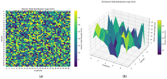
Figure 1.
Example of electric field distribution maps: (a) Example of two dimensional electric field distribution map. (b) Example of three dimensional electric field distribution map.
Within this mathematical framework, various terms are encountered in the literature when referring to this problem. The literature on electric field distribution mapping reveals a striking variety of terms used to describe conceptually similar constructs. Among these are Electric Field Strength Map, Electromagnetic Exposure Map, Electromagnetic Field Exposure Map, Electromagnetic Field Magnitude, Electromagnetic Field Map, and Electromagnetic Pollution Map, all referring to spatial representations of field intensity or exposure. Additionally, terms such as EMF Exposure Map, Path Loss Map, Power Spectrum Map, and Radio Environment Map (REM) are commonly encountered, reflecting variations in focus or application domain. Furthermore, the terminology extends to Radio Map, Radio Map–Path Loss, Radio Network Map, Radio Propagation Map, and Radio Signal Strength Field. All these different terms, which often overlap in meaning and usage, are summarized in Table 1 and Table 2. This diversity underscores a lack of standardization in the field, often leading to confusion and inconsistency across studies, and highlights the need for a unified definitional framework.
2.1.1. Radio Map and Spectrum Cartography
Radio maps are primarily designed to visualize signal characteristics across space, such as received signal strength (RSS), signal-to-noise ratio (SNR), interference power, power spectral density (PSD), electromagnetic absorption, channel gain, and other related metrics. These maps serve as a fundamental tool within the domain of wireless communication, supporting network planning, optimization, and performance analysis. The typical output format is a heat map or a spatial grid of signal values, with common units including dBm, RSSI, and SNR. Radio maps generally provide medium to high spatial resolution and may be constructed either as static representations or time-averaged snapshots, depending on the specific application requirements. Data sources used to generate radio maps include sensor-based measurements, simulation data, and mobile user reports. These maps are used predominantly by engineers, network planners, and system designers to evaluate coverage, identify dead zones, and improve service quality in wireless networks [25]. Spectrum cartography encompasses a comprehensive suite of techniques designed to construct and update radio maps, offering detailed insights into the radio frequency environment. These techniques capture and represent key metrics such as the power of the received signal, the intensity of interference, the spectral density of power, the electromagnetic absorption, and the gain of the channel across geographic areas (Table 1). In practice, spectrum cartography often involves constructing multidomain RF maps spanning dimensions such as frequency, space, and time—using only sparse and incomplete measurement data [9,26,27,28].

Table 1.
Comparison between the terms “Radio maps” and “Spectrum cartography”.
Table 1.
Comparison between the terms “Radio maps” and “Spectrum cartography”.
| Feature | Radio Maps | Spectrum Cartography |
|---|---|---|
| Definition | Static maps of radio signal features | The technique to estimate & construct maps |
| Focus | The map itself | The process of mapping |
2.1.2. Radio Environment Map
The concept of a radio map broadly refers to a spatial representation of the power spectral density (PSD) of wireless signals across geographic, frequency, and temporal dimensions. A more advanced form, the Radio Environment Map, integrates diverse data sources—including geographic information, radio device specifications, propagation models, and real-time spectrum data—to provide a comprehensive cognitive map of the wireless environment. In addition, spatial spectrum databases serve as practical implementations of these concepts, enabling global awareness of spectrum usage. These systems play a pivotal role in applications such as spectrum monitoring, dynamic spectrum access, interference management, and support for adaptive mobile network architectures [29].
A REM aims to capture spectrum usage and contextual environmental information in dynamic and often complex radio environments. It is a core element in cognitive radio systems and dynamic spectrum access frameworks, where understanding the temporal and spatial behavior of spectrum occupancy is essential. REMs are typically structured as databases or spatial maps containing RF metadata, with key metrics such as Signal-to-Interference-plus-Noise Ratio (SINR), occupancy probability, and interference level [30]. These maps maintain a medium to high spatial resolution and are designed to be both dynamic and time-aware, reflecting real-time changes in spectrum activity. Data for REMs are collected through spectrum sensing and network-derived metadata. They are mainly used by cognitive radio agents and spectrum regulators for managing interference, guiding adaptive transmission strategies, and supporting spectrum policy enforcement [25].
2.1.3. Electromagnetic Field Exposure Map
Here, we enter a different field—one at the intersection of public health, medical physics, and radiation protection. In this context, the maps are referred to as electromagnetic field exposure maps. Given the widespread integration of wireless communication systems into modern daily life, the monitoring of associated phenomena, particularly radiofrequency electromagnetic field (RF-EMF) exposure, has become increasingly important. In urban environments, a diverse array of EMF sources, including WiFi networks and cellular technologies such as 5G systems, collectively shape the electromagnetic landscape, necessitating continuous surveillance and assessment.
An EMF Exposure Map is constructed to evaluate and visualize human exposure to electromagnetic field (EMF) radiation. These maps play a vital role in public health assessment and regulatory compliance by providing spatial representations of EMF intensity levels. The application domain includes studies on environmental health, urban planning, and electromagnetic compatibility. EMF exposure maps present their output as detailed spatial intensity distributions, typically using physical units such as volts per meter (V/m), amperes per meter (A/m), or watts per square meter (W/m2). They are known for offering high spatial resolution, particularly in proximity to transmission sources where exposure gradients can be steep. These maps can be generated in real-time or through periodic sampling, using data derived from EMF meters as well as modeled or measured values. They are widely used by health agencies, municipalities, urban developers and academic researchers to monitor exposure levels, inform the public, and support evidence-based regulatory decisions. Generating such maps typically involves extensive and costly measurement campaigns. To optimize these efforts and enhance the representativeness of the resulting exposure maps, systematic criteria must be established for the selection of measurement locations.
The comparative Table 2 highlights that although Radio Maps, REMs, and EMF Exposure Maps all involve spatial representation of electromagnetic phenomena, they serve different purposes across different domains, using different metrics, data sources, and user audiences. Understanding these differences is essential for selecting the appropriate mapping approach based on the intended application, whether for network optimization, dynamic spectrum management, or public health assessment (See Figure 2).
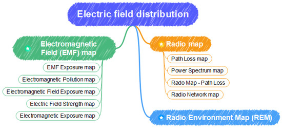
Figure 2.
Conceptual mind map of the terminology used in the literature for spatial representations of electric-field distribution.
Table 2.
Comparison of Radio Map, REM, and EMF Exposure Map: Commonalities and Differences.
Table 2.
Comparison of Radio Map, REM, and EMF Exposure Map: Commonalities and Differences.
| Feature | Radio Map | REM (Radio Environment Map) | EMF Exposure Map |
|---|---|---|---|
| Primary Purpose | Visualize signal characteristics (e.g., RSS, SNR) | Capture spectrum usage and environment context | Assess human exposure to EMF radiation |
| Domain | Wireless communications | Wireless communications | Public health, EMF compliance |
| Output Type | Heatmap or grid of signal values | Database or map with RF metadata | Spatial exposure map with EMF intensity |
| Units/Metric | dBm, RSSI, SNR | SINR, occupancy probability, interference level | V/m, A/m, W/m2 |
| Spatial Resolution | Medium to high | Medium to high | High (especially near transmitters) |
| Temporal Aspect | May be static or time-averaged | Often dynamic and time-aware | Can be real-time or periodic |
| Sources of Data | Sensor measurements, simulation, mobile data | Spectrum sensing, network metadata | EMF meters, modeled or measured values |
| Used By | Network planners, engineers | Cognitive radio agents, regulators | Health agencies, municipalities, researchers |
2.2. Outdoor and Indoor Maps
To continue addressing this complexity, we introduce the terms indoor and outdoor as a first key contextual categories within our broader analysis. These terms reflect the environmental settings in which EMF mapping techniques are applied and serve as fundamental dimensions for interpreting methodological differences. Radio mapping and electromagnetic field exposure mapping varies significantly depending on the environmental context in which it is conducted. The propagation characteristics of electromagnetic signals, the complexity of geograchical background, and the availability of measurements all differ between indoor and outdoor environments (Figure 3). A clear distinction between these contexts is essential for understanding the suitability of different computational and machine learning methods (Table 2).
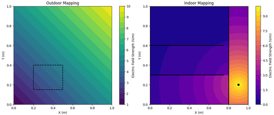
Figure 3.
Spatial Interpolation of Electromagnetic Field Exposure in Outdoor and Indoor Environments.
2.2.1. Outdoor Environment
Outdoor radio mapping or EMF exposure mapping typically involves wide-area scenarios such as urban, suburban, or rural landscapes. The propagation of electromagnetic waves in outdoor environments is influenced by large-scale structures such as buildings, terrain topology and atmospheric conditions. One of the key challenges in outdoor environments is the sparsity of data due to the vast area and the cost of measurement campaigns. This has led to an increased reliance on spatial interpolation and predictive modeling.
2.2.2. Indoor Environment
In contrast, indoor radio mapping or EMF exposure mapping deals with environments where signal propagation is significantly affected by walls, furniture, floors, and other interior elements. The presence of multipath effects, diffraction, and scattering leads to highly complex and variable EMF distributions. This makes traditional modeling approaches less effective unless detailed structural data and advanced ray-tracing techniques are employed. The indoor setting allows for more controlled data collection and finer granularity in exposure mapping.
This contextual differentiation not only helps structure the discussion but also highlights how environmental characteristics influence the selection of computational methods, the modeling assumptions adopted, and the practical challenges encountered in deploying electric field distribution mapping solutions.
2.3. Data Acquisition Methods
2.3.1. In Situ Measurements
In this method, technicians use handheld electromagnetic field metersesearchers to manually measure the field strength at specific locations. These devices include spectrum analyzers with probes or EMF meters. The process is straightforward and cost-effective, making it suitable for small-scale or preliminary surveys. However, it is time-consuming and provides low spatial resolution unless measurements are taken at a high density across the area [31,32].
2.3.2. Wireless Sensor Networks
This method involves the deployment of distributed sensor arrays installed throughout an area. These stationary sensors continuously monitor the electromagnetic field strength over time. The key advantage of this approach lies in its ability to provide long-term and real-time monitoring, which makes it highly suitable for urban environments. Nevertheless, the initial setup cost can be significant, and data is limited to the locations where the sensors are installed [33,34].
2.3.3. Simulation and Model-Based Data—Synthetic Data
Rather than direct field measurements, this method uses computational electromagnetic tools such as ray tracing to predict the distribution of electromagnetic fields. These models are based on known source parameters and environmental configurations. The primary benefit is the ability to estimate field values in inaccessible areas. However, the precision of the simulation depends heavily on the quality of the input data and the degree to which the model is calibrated with real world measurements [35].
2.4. Data Sets
Measurement data is available from the Department of Electronic Communications [36], operating under the Ministry of Research, Innovation, and Digital Policy of Cyprus. The dataset includes measurements from 2017 to the present, with two measurement campaigns conducted annually—one per semester. The methodology involves performing three distinct measurements around each telecommunications site, specifically at locations where electromagnetic radiation exposure is expected to be highest. These points are typically situated at elevated positions near the base stations and aligned with the main signal emission axis. Measurements are taken at different distances to ensure thorough spatial coverage.
Another open data set is provided by the Agence Nationale des Fréquences (ANFR) [37], the French government agency responsible for managing national radio frequencies. ANFR operates accredited laboratories to measure public exposure to radio waves from cell towers and personal devices such as mobile phones. These measurements support public inquiries and contribute to the development of national and international exposure standards. Cartoradio, ANFR’s online mapping tool, displays the locations of relay antennas and electromagnetic field measurements. Users can search by address or area and access detailed measurement reports. Since October 2021, Cartoradio also offers statistics on radio sites, including 5G deployment by region, operator, and frequency band.
Bakirtzis et al. [38] released a comprehensive data set of radio maps generated through ray tracing simulations in indoor environments of varying structural complexity, across multiple frequency bands, and under various antenna radiation pattern assumptions. According to the authors, leveraging this dataset facilitates the development of fully data-driven propagation models capable of generalizing across unseen building layouts, frequency ranges, and antenna configurations—thereby offering a viable path toward replacing traditional radio signal propagation modeling techniques.
Another open-access dataset, known as RadioMapSeer [39,40], is a publicly available collection of radio map datasets generated for dense urban environments. It includes simulated data for path loss, received signal strength (RSS), and time of arrival (ToA) across a wide range of realistic urban scenarios based on actual city maps. The dataset is provided in two configurations: (1) a 2D setting, where transmitters (Tx) are deployed at street level, 1.5 m above ground—matching the height of the 256 × 256 receiver pixel grid; and (2) an extended 3D setting, which incorporates variable building heights and rooftop transmitter deployments. Another dataset creation effort, described in [41], is known as RSRPSet. In this approach, a 320-m by 320-m area is defined based on the location and orientation of the base station’s antenna to represent its effective coverage. This area is then divided into a grid, where each cell corresponds to a 5-m by 5-m region. Similar, the data set, called High-Resolution Radio Environment Map Dataset [42] includes two measured REMs of a corridor in an indoor office environment. These high-resolution maps were generated using a semi-automated setup, where an Automated Guided Vehicle (AGV) equipped with a transmitter followed a predefined path.
2.5. Related Work
Although the literature contains several review articles, they tend to address only narrow sub-fields. Abdulkarim et al. [43] review path loss models in the context of machine learning-based algorithms, with a particular focus on models developed between 2000 and 2021. The study examines network parameters, architectural designs, and the applicability of these models, while also identifying key trends and proposing directions for future research in this evolving field. Li et al. [44], for instance, focus on the concept of radio environment map (REM), summarize recent research progress, and highlight the key challenges involved in constructing accurate spectrum patterns. Phillips et al. [35] present a comprehensive and up-to-date survey of path loss prediction methods, covering over six decades of continuous research in the field. They introduce a novel taxonomy to systematically compare and contrast the wide range of existing approaches, offering a concise yet thorough overview of the methods. In addition, the authors provide valuable insights into emerging trends and outline promising directions for future research. Feng et al. [45] offer a systematic taxonomy of radio map estimation (RME) techniques based on their dependence on prior model knowledge, distinguishing three families, model-driven, data-driven, and hybrid approaches. For each category, they survey representative studies, analyzing strengths and limitations in detail. The authors also compile publicly available radio map datasets and emphasize the importance of mixed simulation-and-measurement corpora for advancing RME research. Dare et al. [46] provide a comprehensive review of the Radio Environment Map (REM) concept, detailing the various layers of information it encompasses, the techniques used for its construction, and key contributions from the existing literature. Romero et al. [9] begin by introducing several representative applications of radio maps, then proceed to examine the most prominent radio map estimation (RME) methods. The discussion progresses from basic regression techniques to more advanced and state-of-the-art algorithms, offering a structured view of the methodological landscape. To aid in understanding this diverse set of tools, the authors also include illustrative toy examples that provide intuitive insight into the functioning of each approach. Kurt et al. [47] present an overview of experimentally validated propagation models for wireless sensor networks (WSNs), offering quantitative comparisons of different models used in WSN research. Their study evaluates these models under various deployment scenarios and frequency bands, providing valuable insights into their relative performance and applicability in real-world WSN environments.
Abbreviations for Table 3: MBML—Model-Based Machine Learning (data-driven predictors that incorporate physical priors); MBI—Model-Based Interpolation (classical spatial-interpolation techniques such as Kriging or IDW guided by propagation models); AM—Analytical Models (closed-form or semi-empirical formulas derived directly from electromagnetic theory).
Table 3.
Comparison of relevant survey papers.
Table 3.
Comparison of relevant survey papers.
| References | Taxonomy Domain | Map Category | Map Construction Method | Dataset Categories |
|---|---|---|---|---|
| [43] | Wireless Communication | - | MBML | - |
| [44] | Wireless Communication | Radio Environment Map | - | - |
| [35] | Wireless Communication | Radio Environment Map | MBI + AM | - |
| [45] | Wireless Communication | Radio Map | MBI + MBML + AM | X |
| [46] | Wireless Communication | Radio Environment Map | MBI + MBML | - |
| [9] | Wireless Communication | Radio Map | MBI + MBML + AM | - |
| [47] | Wireless Communication | - | AM | - |
| Our paper | Wireless Communication | Radio Environment Map | MBI + MBML + AM | X |
| + | Radio Map | |||
| Public Health | EMF Exposure Map |
Compared with previous surveys (Table 3), our review extends the scope of analysis beyond wireless communication to also address the public health domain through the consideration of EMF exposure maps. In addition to covering radio environment maps and radio maps, our paper integrates multiple map construction methods (MBI, MBML, and AM) and discusses dataset categories. This broader taxonomy and interdisciplinary perspective provide a more comprehensive overview of the field and highlight emerging research directions that were not covered in earlier works.
The search and selection process of the reviewed studies is summarized in Figure 4. The systematic search was conducted in the following electronic databases: IEEE Xplore, Scopus, Web of Science, and PubMed. The Boolean query used (adapted to the syntax of each database) was:
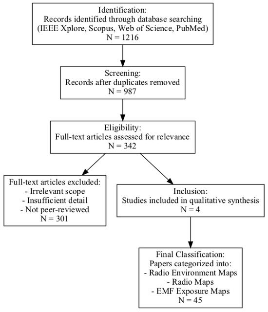
Figure 4.
PRISMA-style flow diagram illustrating the search and selection process of the reviewed studies.
| ("radio map" OR "radio environment map" OR "REM" OR "spectrum cartography" OR |
| "path loss map" OR "electromagnetic exposure map" OR "electromagnetic field map" OR |
| "electric field strength map") |
| AND |
| ("mapping" OR "estimation" OR "prediction" OR "machine learning" OR "computational model") |
A total of N = 1216 records were initially identified from major databases (IEEE Xplore, Scopus, Web of Science, and PubMed). The inclusion criteria required that studies be peer-reviewed journal articles or conference papers, focusing explicitly on radio maps, radio environment maps, or electromagnetic field (EMF) exposure maps. Eligible works employed analytical models, model-based interpolation, or data-driven and machine learning approaches for field distribution mapping. Only studies published in English and providing methodological contributions—such as the construction, estimation, or validation of EMF or radio maps—were considered.
Conversely, exclusion criteria applied to papers not directly related to electromagnetic field distribution mapping, non peer-reviewed sources such as reports, theses, or white papers, and publications in languages other than English. Articles without accessible full text were excluded, as were studies focusing exclusively on hardware design, antenna optimization, or unrelated RF applications without a mapping component.
After removing duplicates, N = 987 records remained. Screening based on title and abstract resulted in N = 342 full-text articles assessed for eligibility. Following the application of inclusion and exclusion criteria, a final set of N = 45 studies was retained and categorized into three groups: radio environment maps, radio maps, and EMF exposure maps.
This section established a clear conceptual and mathematical framework for electromagnetic field distribution mapping, addressing the fragmented and overlapping terminology found in previous literature. By systematically distinguishing between radio maps, radio environment maps, and EMF exposure maps, as well as differentiating indoor and outdoor mapping contexts, our work provides a unified foundation for subsequent methodological analysis. Furthermore, we reviewed the main data acquisition techniques and open-access datasets, which are essential for developing, benchmarking, and validating mapping methods. Unlike earlier studies that focus narrowly on either wireless communication or public health, this integrated framework—encompassing terminology, environmental context, and datasets—bridges both domains, offering a structured basis for comparing approaches and guiding future research in a standardized and reproducible manner.
3. Electric Field Distribution Maps Construction Methods
3.1. Analytical Expressions for Radio Map Construction
The concept of analytical expressions for radio map construction is based to the construction of the path loss function, which characterizes the attenuation of an electromagnetic wave as it propagates through space. Specifically, path loss denotes the reduction in wave power density experienced due to factors such as distance, obstacles, and environmental conditions [23]. We refer to it as the path loss function because, in the literature, these methods are specifically designed to address signal attenuation problems in wireless communication and are not typically applied in other domains. The models discussed here are a priori in nature, meaning that they rely solely on predefined parameters and theoretical assumptions, without incorporating direct measurement data in their predictions. The path loss function is a function that models the attenuation of a radio signal as a function of distance d between the transmitter and receiver.
We begin with the Free-Space Propagation Model, which represents the simplest scenario of electromagnetic wave propagation under ideal line-of-sight conditions. It is governed by the Friis transmission equation [48], relating the received power to the transmitted power , antenna gains , , wavelength , and the distance r between antennas:
Although useful for initial estimations and theoretical analysis, the free-space model neglects environmental effects such as reflection and diffraction, which are often significant in real deployments. To account for such effects, the Two-Ray Reflection Model extends the free-space formulation by including a reflected path from the ground. This model provides more realistic estimates for scenarios that involve large transmitter-receiver separation and flat reflective surfaces. It is particularly applicable to outdoor line-of-sight conditions, where ground reflection can substantially alter the signal strength. The complete mathematical formulation is provided in the Appendix A. Building on these deterministic approaches, empirical models such as the Egli Model offer practical alternatives based on measured data. Designed for point-to-point communication in urban and rural settings, the Egli model operates in the UHF and VHF bands (30 MHz to 3 GHz) and considers parameters such as distance, frequency, and antenna heights. It is especially useful when detailed environmental modeling is impractical. For its mathematical expression, see Appendix B. Finally, the Hata Model, an extension of the Okumura model [35], is one of the most widely adopted empirical models for outdoor mobile communication. Applicable to frequencies from 150 MHz to 1500 MHz, it provides correction factors for urban, suburban, and rural environments. Its reliability and simplicity have made it a standard in mobile network planning. Detailed equations and parameterizations are available in Appendix C.
Figure 5 consists of the flowchart illustrating the analytical approach, where electromagnetic field distributions are computed directly from input parameters (frequency, transmitter configuration, environment type) using propagation models, yielding grid-based EMF maps.
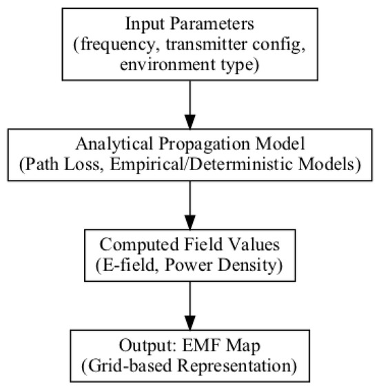
Figure 5.
Analytical models for EMF mapping.
The authors in [49] modeled a single narrowband WiFi transmitter using the log-distance path loss model (LDPL). The study in [50] shows that satellite images of buildings and the adjacent spaces can be used effectively to estimate path loss model coefficients for signal propagation along straight, level urban streets. Using easily accessible environmental parameters, the proposed models enable accurate path loss predictions and support the development of efficient node placement strategies to ensure comprehensive urban coverage. The work presented in [51] offers a detailed analysis of large-scale path loss in wireless networks operating under the IEEE 802.11 g standard [51] at 2.4 GHz, considering both indoor and outdoor environments. The authors propose a new propagation model and conduct a comparative evaluation against existing models. In addition, the study examines the impact of environmental factors, specifically temperature and relative humidity, on signal attenuation. Rizk et al. [52] investigate the application of diffraction theory and geometrical optics to model radio wave propagation in microcellular urban environments. The proposed model adopts a simplified two-dimensional (2D) representation, where building walls are modeled as line segments and buildings are assumed to be of infinite height. Despite this abstraction, the model is capable of handling arbitrary building layouts through an efficient algorithm, which is briefly outlined in the paper.
3.2. Model-Based Radio Map Estimation
According to [25], a radio map is generally characterized by a function that maps a 3-tuple variable to the signal power, denoted by , where represents the location in a three-dimensional Cartesian coordinate system, and f and t denote the frequency point and time instant, respectively. This is a subcase of Equation (1), where and , with F denoting the frequency domain and T the time domain.
This definition of a radio map builds upon the foundational framework introduced in [53], and it has been extended to encompass a broader range of scenarios. The radio map is modeled as a function of frequency f and geographic location , and is expressed as:
where n is the number of transmitters, represents the channel power gain from the i-th transmitter, and denotes its power spectral density (PSD) [25]. The channel gain may be explicitly specified based on prior knowledge relevant to specific applications or estimated through sensor data.
In [54], the authors introduce a spline-based methodology for electromagnetic field estimation, utilizing a basis expansion model wherein the field is represented as a combination of known basis functions weighted by unknown coefficients. These coefficients are inferred from noisy field samples. The proposed spline-based framework is particularly motivated by applications in spectrum cartography, where a collection of cognitive radios cooperatively estimate the spatial and spectral distribution of RF power. Sato et al. [55] propose a novel method for radio map construction that performs simultaneous interpolation of received signal power across both spatial and frequency domains. The approach leverages the observation that shadowing effects exhibit strong correlation over a wide frequency range. The key idea is to utilize shadowing values measured at various frequencies as proxies for those at the target frequency. Using real-world datasets collected at 870, 2115, and 3500 MHz within a cellular network, the authors demonstrate that their method can accurately generate radio maps, even when little or no data is available at the target frequency.
3.3. Model-Free Radio Map Reconstruction Interpolation-Geospatial Based Methods
In contrast to model-based approaches, model-free methods do not rely on predefined propagation models, but instead use spatial neighborhood information. Broadly, model-free techniques can be classified into two categories: interpolation-based methods and learning-based methods, as outlined below.
Interpolation-based methods and machine learning techniques such as k-nearest neighbors (k-NN) approximate the electromagnetic field distribution at a given location by combining measurements from neighboring points. This can be mathematically expressed as:
where denotes the observation from the i-th sensor, and represents the associated combination weight [25,53]. A representative example is inverse distance weighted (IDW) interpolation, where the power gain is inversely proportional to the distance between the transmitter and receiver. This structure is mathematically analogous to the classical weighted mean , where is a function defined over a set and is a non-negative weight function. In this context, the spatial weights in the radio map equation play the same role as the weight functions in interpolation theory, such as the Sibson or Laplace weight functions [23]. Beyond linear interpolation, more sophisticated alternatives include radio basis function (RBF) interpolation, where various kernels such as Gaussian Kriging, multiquadrics, or splines are employed. Among these, ordinary Kriging is a classical interpolation technique that optimizes the power spectral density (PSD) by minimizing the variance of estimation errors. Classical interpolation approaches typically assume that each observation influences the surrounding surface only within a certain distance.
Figure 6 consists of the flowchart of the interpolation approach, which uses sparse measurement samples and spatial interpolation methods (e.g., Kriging, IDW, Sibson) to estimate field values at unsampled locations and generate a continuous EMF map.
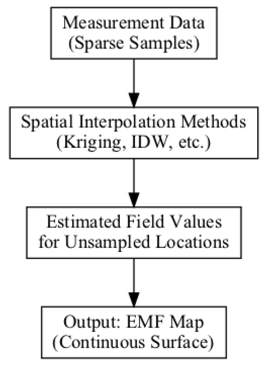
Figure 6.
Model-based interpolation for EMF mapping.
In [56], a hybrid approach is proposed that combines kriging-based spatial interpolation and recurrent neural networks for temporal prediction. This framework estimates spectrum occupancy probabilities using empirical measurements in cellular cognitive radio (CR) networks. The analysis in [57] evaluates spatial interpolation methods, such as Inverse Distance Weighting (IDW), for indoor radio information field (RIF) estimation. The study demonstrates robust and reliable performance in a prototype REM setting. In a case study conducted in Caracas, Venezuela, ref. [58] investigates interpolation methods for mapping EMF magnitudes. The authors compare SPLINE, IDW, and Kriging, finding IDW to offer the most accurate estimates across the pilot area. Three spatial interpolation techniques for estimating radio environments are compared in [59], with simulations performed for both indoor and outdoor scenarios. The results highlight trade-offs in accuracy and reliability among the methods. Finally, ref. [60] presents a geostatistical modeling approach applied to a 2.5 GHz WiMax network. The study evaluates robust techniques for radio environment and coverage mapping, validated through a case study at the University of Colorado, Boulder. Interference cartography is introduced in [61] as a means to detect and utilize spectrum opportunities in secondary usage scenarios. The method combines geo-located measurements from various network entities and applies spatial interpolation to estimate interference levels across a target area. Finally, Guillén-Piña et al. [62] employ evolutionary computation to identify an optimal subset of measurement points for constructing high-quality electromagnetic field exposure maps—minimizing error with respect to a reference map—and demonstrate that accurate exposure maps can be achieved with significantly fewer samples. Panagiotakopoulos et al. [63] aim to determine the most effective geospatial interpolation method for constructing electromagnetic field strength maps in large-scale urban environments. The study evaluates five interpolation techniques: four based on Gaussian Process Regression (Kriging) and one using the classical inverse-distance weighted average of nearest neighbors. Using a dataset of 3632 EMF measurements collected across the city of Paris, the authors demonstrate that Kriging—particularly with the exponential variogram model—offers superior performance in capturing spatial autocorrelation compared to the nearest-neighbor approach. Additionally, the removal of outliers was found to significantly enhance the performance of all models, reducing both the mean squared error (MSE) and prediction variability. Also, Kiouvrekis et al. [64] compared five methods for mapping nationwide electric-field strength (30 MHz–6 GHz) using 3621 measurements over 9251 km2. Gaussian-process (Kriging) models generally produce the most accurate spatial predictions, but when outliers are removed, a simple weighted nearest-neighbor approach performs almost as well. This suggests that both advanced Kriging and classical neighbor techniques can be effective, depending on data quality.
In [65] the authors proposed a methodology for assessing electromagnetic-field exposure over large areas. It is demonstrated in an urban zone of 2.8 km2 within a 35.11 km2 municipality, with both rural and urban settings being considered. To limit the sampling density, the authors introduce line-of-sight criteria to identify relevant emitters. In the urban case study, they estimate that 8–10 measurement points per square kilometer are sufficient.
3.4. Model-Free Radio Map Reconstruction Machine Learning Based Methods
In this case, the situation is more akin to a black-box modeling approach, where no explicit analytical expression for the electromagnetic field distribution is available. Instead, the mapping is learned directly from data using machine learning techniques. The radio map can therefore be expressed as:
where denotes a regression function approximated by a data-driven model, such as a neural network, random forest, or Gaussian process regression, trained on a set of sensor observations. Here, represents the i-th sensor location or measurement or characteristic vector, f is the frequency, and t is the time instance.
Instead of relying on predefined rules or neighborhood structures like model-based and interpolation approaches, black-box models directly infer complex spatial and spectral relationships from the data, proving useful in dynamic or hard-to-model settings.
Figure 7 consists of the flowchart showing the data-driven approach, where measurements and contextual features are used to train machine learning models (e.g., Random Forests, XGBoost, CNNs, GANs) that learn the mapping between features and field strength, enabling prediction of EMF maps for new locations and conditions.
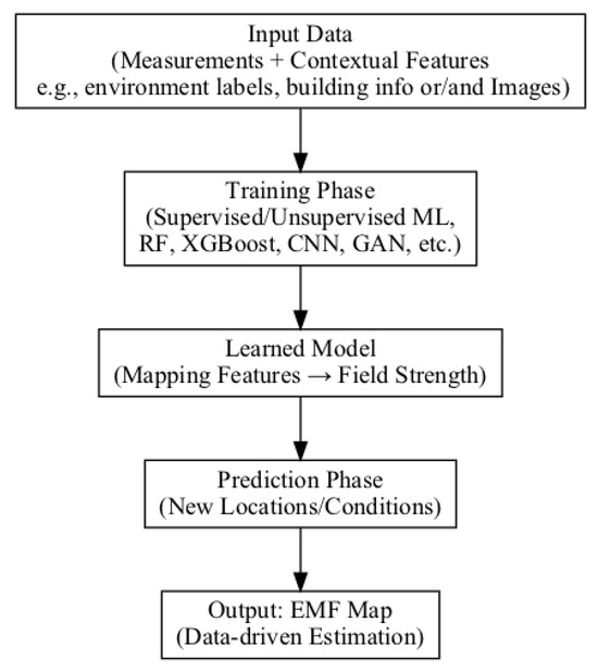
Figure 7.
Machine learning approaches for EMF mapping.
The study in [66] introduces a disaggregated emitter radio map approach, where deep neural networks (DNNs) model the radio maps of individual emitters. This framework mitigates learning and generalization challenges and incorporates a two-stage spectrum cartography (SC) method that combines non-negative matrix factorization and an optimized iterative algorithm. Theoretical contributions address recoverability, sample complexity, and robustness to noise, properties that are not often formally established in the completion of the deep learning-based radio tensor. In [67], a limited feedback-based SC framework is proposed, which incorporates a deep generative adversarial network (GAN) based on deep feedback to mitigate the effects of heavy shadowing. Unlike conventional real-valued feedback strategies, the authors adopt a random quantization technique with a maximum likelihood estimation (MLE) criterion, theoretically proving radio map recoverability under certain conditions and validating performance through simulations.
Chaves-Villota et al. [68] introduced DeepREM, a framework comprising two deep learning models—U-Net and cGAN—designed to estimate radio environment maps (REMs) from sparse measurement data, without the need for any supplementary information. In [53], a two-phase learning framework for radio map estimation (RME) is developed by combining a conventional propagation model with a conditional GAN (cGAN). The method leverages global propagation patterns and local shadowing features to optimize the generative model, demonstrating improved accuracy in outdoor environments with scarce data.
The work in [69] presents a spectrum cartography algorithm to estimate power spectrum distributions in wide frequency bands. The algorithm is based on a nonparametric regression framework, leading to a support vector machine (SVM) formulation. Simulations show that the method yields accurate maps using a simplified sensing architecture with reduced feedback. In [70], DNNs are used to predict the strength of radio signals in urban environments. The model incorporates sampled signal strengths and 3D environmental data to account for wave scattering effects, enhancing spatial prediction accuracy. The authors of [6] propose a deep learning model, RadioUNet, to estimate the propagation path loss between arbitrary transmitter-receiver pairs. The model is trained on a simulation dataset and significantly reduces computation time compared to traditional simulation tools, maintaining high accuracy. To address the challenges in cognitive radio networks, Ref. [71] presents MEGANs, a GAN-based algorithm to estimate power spectrum maps (PSMs). Unlike traditional approaches that rely on predefined propagation assumptions, MEGANs learns propagation features directly, yielding more accurate spectrum estimations.
The paper in [72] introduces a deep-complete autoencoder architecture to estimate radio occupancy maps with fewer measurements by learning spatial propagation characteristics. This is the first reported use of DNNs in this context, demonstrating substantial measurement reduction while maintaining accuracy. In [73], a hybrid algorithm is proposed that combines estimators of deep neural networks and traditional models, addressing the trade-off between performance and data requirements. The study emphasizes the potential of combining learning-based and classical approaches to improve efficiency and accuracy. RecNet, a neural network designed to reconstruct fine-grained radio maps, is introduced in [74]. Imagining reconstruction as a super-resolution task, the model generates high-resolution maps from low-resolution data, reducing the error by more than 20% compared to recent algorithms. In [6], the authors propose RadioUNet, a deep neural network trained on simulation data to estimate path loss in urban environments. The model delivers high accuracy while significantly reducing computation time, making it suitable for real-time use.
In [75], the authors conducted field measurements in an urban environment to collect geographic and network-related data from receiving mobile equipment and to assess path loss for radio signals transmitted at 189.25 MHz and 479.25 MHz. Multiple artificial neural network (ANN) models were developed and trained, exploring different input parameter combinations, network architectures, activation functions, and learning algorithms. The aim was to accurately predict path loss values under varying conditions. Model performance was rigorously evaluated using several statistical indicators, including Mean Absolute Error (MAE), Mean Squared Error (MSE), Root Mean Squared Error (RMSE), Standard Deviation (SD), and the Regression Coefficient (R), providing a comprehensive assessment of prediction accuracy. In [76], a federated learning model called RadioSRCNet is proposed, incorporating super-resolution techniques for prediction of pathloss. Users locally train the model while a Unmanned aerial vehicle (UAV) aggregates non-sensitive data. The approach balances resolution and computational overhead through an Arbitrary Position Prediction (APP) module.
A transfer learning framework is proposed in [77] to reconstruct radio maps for different antenna tilt configurations. By transferring knowledge between configurations, the model achieves high accuracy with minimal or no new measurements, outperforming traditional machine learning methods. The work in [78] evaluates artificial neural networks (ANNs) for the prediction of macrocell pathloss, comparing them against the ITU-R P.1546 and Okumura–Hata models. The results indicate that ANNs can outperform classical models in certain terrain conditions. A convolutional neural network (CNN)-based propagation prediction model is introduced in [79]. The paper details model architecture and input mapping, demonstrating improved accuracy in modeling complex propagation patterns. Deep learning techniques incorporating satellite imagery are used in [80] to model channel characteristics. The proposed model is benchmarked against ray-tracing and stochastic approaches, with results showing competitive performance. In [81], the authors introduce FadeNet, a CNN-based model for large-scale fading prediction.
Using topographical features as input, FadeNet achieves root mean square error as low as 5.6 dB across millimeter-wave deployments in multiple cities. Kiouvrekis et al. [82] present an explainable machine learning framework for predicting electric field strength across urban, semi-urban, and rural areas in Cyprus. The model is trained on 6543 EMF measurements collected in 2023 from mobile and digital TV stations. The dataset includes geospatial and environmental features such as antenna distance, population density, urbanization level, and building characteristics. Several models—kNN, neural networks, decision trees, random forests, XGBoost, and LightGBM—were evaluated using a two-semester split. Explainable AI analysis identified antenna distance, building volume, and population density as key predictors of EMF intensity. In [83], the authors propose a novel framework for indoor radio map construction that integrates image sensing, 3D reconstruction, deep learning, and ray tracing. The approach models indoor environments using RGB-D images, representing structural information as a set of cuboids. By converting room materials and obstacles into vector data, the method enables accurate ray-tracing simulations based on detailed indoor geometry.
Zhang et al. [84] propose a deep learning framework for predicting electric field (E-field) levels in complex urban environments. The study begins by describing the measurement campaign and publicly available databases used to construct the training dataset, including a detailed explanation of how these datasets are processed and integrated to optimize their compatibility with Convolutional Neural Network (CNN)-based models. The authors then introduce the proposed model, ExposNet, and provide a comprehensive description of its network architecture and operational workflow. Nyakyi et al. [85] conducted measurements of power density levels at various locations in Dodoma, Dar es Salaam, and Mwanza—areas characterized by high population density—to assess RF-EMF exposure. To estimate the total power density at different sites, the authors developed predictive models based on Artificial Neural Networks (ANN) and Multiple Linear Regression (MLR), using data from multiple RF-EMF sources.
Xiangyu et al. [86] introduce DeepMap, a deep Gaussian process framework designed for indoor radio map construction and location estimation. The proposed method aims to enhance the accuracy of WiFi-based localization, which remains one of the most widely used positioning techniques due to the broad availability of WiFi infrastructure and its cost-effectiveness. In [79], the authors propose a radio propagation prediction model based on deep learning using convolutional neural networks (CNNs). The study provides a detailed explanation of the model and evaluates its performance by analyzing the influence of map-related input parameters on the CNN’s predictive behavior. Seretis et al. [87] develop generalizable models for indoor radio wave propagation capable of predicting received signal strength in previously unseen environments. Their approach supports varying transmitter and receiver positions, as well as different operating frequencies. The study demonstrates that a convolutional neural network (CNN) can effectively learn the underlying physics of indoor propagation from ray-tracing simulations of a limited set of training geometries, enabling it to generalize to substantially different layouts.
In [88], the authors constructed a detailed electric field strength map of urban Paris by evaluating 410 machine learning models based on k-nearest neighbors, neural networks, and decision trees. This extensive analysis enabled the optimization of model performance for accurate EMF predictions. SHAP analysis revealed that building volume around antennas is the most influential feature in the kNN model, followed by population density. In [89], the authors propose a conditional generative adversarial network (cGAN)-based approach to reconstruct electromagnetic field exposure maps using sparse sensor data in outdoor urban environments. The model learns to estimate propagation characteristics based on the surrounding topology. When compared with simple Kriging, the cGAN-based method demonstrated superior accuracy, highlighting its potential as a reliable solution for EMF exposure map reconstruction.
Kiouvrekis et al. [90] conducted a large-scale analysis involving 566 machine learning models across eight French cities, employing six core approaches: k-Nearest Neighbors, XGBoost, Random Forest, Neural Networks, Decision Trees, and Linear Regression. Ensemble methods like Random Forest and XGBoost outperformed other models in predictive accuracy, while simpler models such as Decision Trees and k-NN provided competitive yet slightly less precise results. Neural Networks showed potential for further refinement. All machine learning models significantly outperformed the linear regression baseline. SHAP analysis also revealed notable differences in feature importance rankings between tree-based methods and other model types. M. Mallik et al. [91] propose an algorithm for estimating electromagnetic field exposure maps using a U-Net-based convolutional neural network. The task is formulated as an image reconstruction problem, where each pixel represents received power intensity. The model learns indoor wireless propagation characteristics, accounting for varying positions of Wi-Fi access points. Results demonstrate that realistic indoor environments can be effectively modeled from data, enabling accurate power map estimation.
Also, Kalatzis et al [92] apply explainable-AI (XAI) techniques to the spectral analysis of electromagnetic-field (EMF) measurements collected across Cyprus in the 30 MHz–6 GHz range. The data set combines emissions from mobile telephony, radio broadcasting, and terrestrial digital television, covering FM radio (87.5–108 MHz); VHF and UHF television; and mobile bands at 700, 800, 900, 1800, 2100, 2600, and 3600 MHz—capturing both legacy and emerging wireless technologies. Six machine-learning algorithms (XGBoost, LightGBM, Random Forests, k-nearest neighbours, neural networks, and decision trees) were evaluated for predictive performance in each band. SHAP (Shapley Additive Explanations) was then used to quantify how spatial and demographic factors influence EMF intensity. Ensemble tree models, particularly Random Forests and LightGBM, consistently delivered the highest accuracy and interpretability. SHAP analysis revealed distinct exposure patterns tied to urban form, population density, and built-environment metrics. This XAI-based framework enables data-driven EMF-exposure mapping to support infrastructure planning, compliance monitoring, and public-health risk assessment.
The tables below (Table 4, Table 5 and Table 6) provide the taxonomy based on computational methods. Neural network architectures, including NN, and CNN, are widely used for spatial prediction and interpolation. Generative models such as GANs and cGANs are used for sparse data reconstruction and adversarial learning. Statistical methods such as kriging, inverse distance weighting (IDW), and spline interpolation remain fundamental in many model-based studies. Several works also employ ensemble learning strategies, combining models such as random forests, XGBoost, and k-nearest neighbors. Hybrid approaches, for instance those blending kriging with Gaussian models or neural networks, exemplify efforts to integrate physical knowledge with data-driven inference. The methodological diversity reflects the interdisciplinary nature of EMF mapping research, which brings together expertise from geostatistics, machine learning, and wireless communications.
Table 4.
Summary of studies that employ closed-form analytical expressions for radio-map construction.
Table 4.
Summary of studies that employ closed-form analytical expressions for radio-map construction.
| Reference | Taxonomy Domain | Map Category | Construction Method–Models–Tools | Environment | Dismnsion of the Map | Units of Metric |
|---|---|---|---|---|---|---|
| [49] | Wireless Communication | Radio Map | Analytical expressions for radio map construction | Indoor | 2D | Mean Distance Error in meter |
| [50] | RMSE in dB | |||||
| [51] | RMSE in dB | |||||
| [52] | Outdoor | Mean error in dB |
Table 5.
Summary of studies that employ model-free radio map based to interpolation geospatial methods for radio-map construction.
Table 5.
Summary of studies that employ model-free radio map based to interpolation geospatial methods for radio-map construction.
| Reference | Taxonomy Domain | Map Category | Construction Method–Model–Tools | Dataset Acquisition | Environment | Dismnsion of the Map | Units of Metric |
|---|---|---|---|---|---|---|---|
| [58] | Public Health | Map | Model-free radio map reconstruction interpolation geospatial based methods. | Measurement points | Outdoor | 2D | MAE and MSE in V/m |
| [62] | Electromagnetic field exposure maps | Logarithm of sum of absolute differences in V/m | |||||
| [63] | RMSE in V/m | ||||||
| [64] | RMSE in V/m | ||||||
| [65] | Absolute error in V/m | ||||||
| [57] | Wireless Communication | Radio environment map | Model-free radio map reconstruction interpolation geospatial based methods. | Indoor | MAE in dB | ||
| [59] | Outdoor and Indoor | Relative Mean Absolute Error | |||||
| [60] | Outdoor | Mean RMSE in dB | |||||
| [61] | - | - | - | Mean error in dBm |
Table 6.
Summary of studies that employ model-free radio map based machine learning methods for radio-map construction.
Table 6.
Summary of studies that employ model-free radio map based machine learning methods for radio-map construction.
| Reference | Taxonomy Domain | Map Category | Construction Method–Models–Tools | Dataset Acquisition | Environment | Dismnsion of the Map | Units of Metric |
|---|---|---|---|---|---|---|---|
| [67] | Wireless Communication | Radio Map | Model-free radio map reconstruction machine learning based methods. | Measurement points | - | 2D | LNMSE |
| log-domain normalized mean square error | |||||||
| [69] | spectrum distribution | MSE | |||||
| [72] | Radio Map | RMSE | |||||
| [74] | Wireless Communication | Radio Map | Model-free radio map reconstruction machine learning based methods. | Measurement points | Indoor | Mean RSSI Difference | |
| [83] | Images | RMSE | |||||
| [86] | Measurement points | Mean Distance Error, Mean training error | |||||
| [87] | - | Map data | Outdoor | RMSE | |||
| [68] | Wireless Communication | Radio environment map | Model-free radio map reconstruction machine learning based methods. | DeepREM dataset | Outdoor | RMSE | |
| - | |||||||
| Images | And | ||||||
| - | |||||||
| MAE | |||||||
| [76] | Radio Map | Images | Outdoor | normalized mean squared error (NMSE) | |||
| [79] | - | Measurement points | RMSE | ||||
| [80] | Satellite images | RMSE | |||||
| [81] | Images | RMSE | |||||
| [66] | Wireless Communication | Radio Map | Model-free radio map reconstruction machine learning based methods. | Measurement points | Outdoor | Squared Reconstruction Error | |
| [70] | - | Model-free radio map reconstruction machine learning based methods. | Measurement points and #D model of environment | Mean absolute error | |||
| [71] | Power Spectrum Map | Images + distribution functions | average image reconstruction error | ||||
| [73] | Radio Map | Measurement points | RMSE | ||||
| [75] | - | RMSE, MSE, MAE | |||||
| [77] | Radio Map | MAPE | |||||
| [78] | - | average total hit rate error (AHRE) | |||||
| [82] | Public Helath | Radio Environment Map | Model-free radio map reconstruction machine learning based methods. | Measurement points | Outdoor | RMSE | |
| [84] | Exposure maps | Images | RMSE and MAPE | ||||
| [85] | - | Measurement points | R squared and MSE | ||||
| [88] | - | Images | Indoor | - | |||
| [89] | Electric Field Strength Map | Measurement points | Outdoor | RMSE | |||
| [90] | Electromagnetic Field Exposure Map | Measurement points and Images | structural similarity index (SSIM) | ||||
| [91] | Electric Field Strength Map | Measurement points | RMSE | ||||
| [92] | EMF Exposure Map | sensor measurement map images | Indoor | - | |||
| - | |||||||
| Average SSIM | |||||||
| [93] | Electric Field Strength Map | Measurement points | Outdoor | RMSE |
In this section, we reviewed three primary methodological families for EMF mapping: analytical models, model-based interpolation techniques, and machine learning-driven approaches. While earlier reviews typically concentrate on a single category—often analytical or geospatial methods—our taxonomy captures the full methodological spectrum, including state-of-the-art deep learning models and hybrid techniques that merge physical modeling with data-driven inference. This comprehensive perspective highlights the evolution from traditional propagation models toward adaptive, intelligent systems, underscoring the novelty of our work in unifying these diverse approaches and revealing new opportunities for interdisciplinary applications in both wireless network optimization and public health exposure assessment.
4. Discussion
The analysis presented in this review highlights several key trends shaping the current landscape of electromagnetic field (EMF) exposure mapping. First, there is a notable transition from classical analytical propagation models toward more sophisticated, data-driven approaches, particularly those leveraging machine learning and deep learning techniques. These modern methodologies offer significant advantages in terms of adaptability, accuracy, and the ability to handle complex, dynamic environments where traditional approaches often fail.
Another important observation is the substantial variation in terminology used across studies, including terms such as “radio map,” “path loss map,” “electromagnetic exposure map,” and “electric field strength map.” This diversity underscores the existing ambiguity and frequent overlap in definitions within the field. Establishing a unified and consistent definitional framework, as proposed in this review, is crucial to advance both academic research and practical applications.
An important distinction must be made between single-source, single-frequency mapping and multi-band exposure surveys. The former is typically motivated by engineering needs, such as optimizing coverage and capacity in wireless networks, and can often be addressed with established propagation models. By contrast, exposure surveys that span multiple sources and frequency bands are vastly more complex, as they must capture the aggregate contribution of heterogeneous transmitters operating simultaneously in dynamic environments. This challenge is further amplified in public health studies, where assessments often require not only cross-band exposure levels at a given point in time but also historical trends to support epidemiological analyses. Developing methods that can integrate such spatial, spectral, and temporal dimensions remains an open and pressing research direction.
In addition, the review emphasizes the distinct methodological considerations necessary for indoor versus outdoor environments. Outdoor EMF mapping typically involves dealing with sparse data, large-scale geographic areas, and environmental variables such as terrain and atmospheric conditions, often necessitating predictive modeling and interpolation. In contrast, indoor mapping presents challenges due to complex signal propagation patterns influenced by building structures and interior elements, highlighting the need for advanced ray tracing and detailed structural modeling techniques.
The comprehensive taxonomy presented in this review categorizes EMF mapping methodologies effectively, providing clarity regarding current practices and identifying existing knowledge gaps. Although computational techniques, including interpolation and kriging methods, remain foundational, rapid advancement in machine learning methodologies, such as neural networks and generative adversarial networks (GANs), indicates a strong direction for future research. Specifically, hybrid models that combine traditional physical models with machine learning show promise, as they can potentially leverage the strengths of both approaches.
Based on the results, the imbalance in domain taxonomy suggests that scientific effort remains chiefly motivated by network design and optimization, with comparatively less emphasis on exposure assessment for epidemiological or regulatory purposes. A stronger integration of exposure mapping with public health research could provide valuable evidence for epidemiological studies and inform risk communication efforts.
Machine-learning techniques are the predominant construction approach, accounting for roughly two thirds of the corpus, while interpolation-based geospatial models contribute a further quarter and purely analytical formulations less than ten per cent. The dominance of data-driven ensembles reflects the availability of powerful regressors and open-source frameworks, but it also raises questions of transparency and generalisability, particularly when comparative baselines are sparse. There is room for hybrid paradigms that combine the physical grounding of analytical models with the flexibility of learning algorithms.
Direct measurement remains the chief data source, representing about sixty-two per cent of studies. Image-based or remotely sensed data now supply close to thirty per cent, highlighting growing interest in fast, low-cost sampling surrogates. Around ten per cent of papers (formerly blank, now labelled input of analytical methods) rely on look-up parameters or synthetic data instead of empirical observations. As image repositories expand and photogrammetric tools mature, the relative weight of the Images category can be expected to rise, potentially reducing deployment costs and enabling large-scale exposure mapping.
Two-dimensional outdoor scenarios dominate: two thirds of the investigations concentrate exclusively on outdoor propagation, twenty-one per cent examine indoor exposure, and the remainder either combine the two or leave the field undefined. No study in the present sample produces an explicit three-dimensional map, even though multilayer urban environments are known to exhibit strong vertical gradients. Expanding empirical coverage to complex indoor venues, high-rise districts and mixed-use neighbourhoods would markedly improve the ecological validity of exposure models.
The results underscore a pronounced technical tilt in the field. Most contributions are rooted in wireless-communication engineering, whereas public-health–oriented work occupies a noticeably smaller—but still significant—niche. No additional thematic branches surfaced, suggesting that EMF-mapping research remains anchored in these two primary motivations.
Turning to terminology, the landscape is strikingly fragmented. A sizeable subset of authors leaves their maps without any formal label, hinting either at implicit understanding within sub-communities or at a lack of consensus. Among the studies that do assign a name, “Radio Map” clearly dominates, with “Radio Environment Map” following behind. Labels such as “Electromagnetic-field exposure map” and “Electric-field-strength map” form a middle tier, while an eclectic mix of eight additional terms appears only sporadically, forming a long semantic tail. This dispersion complicates literature searches and reinforces the need for a standardised vocabulary.
With respect to construction methodology, machine-learning pipelines overwhelmingly lead the way. Classic geostatistical interpolation holds a respectable but secondary position, whereas purely analytical formulations now occupy the margins. The methodological hierarchy thus mirrors a broader trend across applied electromagnetics, where data-driven surrogates increasingly supplant first-principles solvers when speed and adaptability matter.
Examining how data are gathered, on-site field measurements remain the dominant evidence base. Remote imagery—be it satellite, aerial, or street-level—constitutes a robust alternative that is gaining traction, especially as open geo-datasets expand. In contrast, studies that forego empirical inputs altogether and rely on synthetic parameters or look-up tables represent only a small minority, underscoring the community’s preference for measurement-anchored validation.
Finally, the environmental taxonomy reveals that outdoor propagation scenarios attract the lion’s share of attention. Indoor deployments form a smaller, but vibrant cluster, reflecting the growing importance of connectivity in buildings. Mixed indoor–outdoor studies are still rare, and a nontrivial set of articles leaves the operational setting vague, an omission that limits reproducibility and comparability between studies.
From an evaluative perspective, recent evidence suggests that ensemble learning methods such as Random Forests and XGBoost, together with deep learning hold particular promise for advancing EMF mapping. These approaches are effective in capturing non-linear spatial patterns, reconstructing sparse datasets, and enabling scalable predictions across complex environments. However, their adoption also faces limitations: ensemble models often sacrifice interpretability, while deep learning frameworks typically require extensive training data and risk reduced generalizability when applied across different urban or regulatory contexts. Beyond the engineering perspective, there remains a notable gap in the public health application of field mapping. Addressing this requires research that systematically integrates multi-band, multi-source assessments with temporal and historical dimensions of exposure, thus strengthening the evidentiary base for epidemiological studies and regulatory decision-making.
A key avenue for future research lies in the systematic comparison of methods for assessing total RF exposure in urban environments. Measurement-based campaigns, simulation-driven approaches, and machine learning models each present distinct trade-offs: direct measurements offer high reliability but are costly and labor-intensive; simulations provide scalability but often rely on simplifying assumptions; and data-driven models can capture complex dynamics at lower cost but may suffer from generalization challenges. A comparative framework that evaluates these approaches in terms of cost, accuracy, scalability, and limitations would be highly valuable for guiding both urban network planning and public health assessments.
5. Conclusions
This review has presented a comprehensive and structured synthesis of methodologies for electromagnetic field (EMF) exposure mapping, spanning analytical models, interpolation techniques, and machine learning approaches. Unlike previous surveys that focus primarily on wireless communication engineering, our work integrates perspectives from both communication networks and public health, thereby broadening the scope and societal relevance of EMF mapping research. A unified taxonomy was proposed to clarify the fragmented terminology in the field, distinguishing among radio maps, radio environment maps, and EMF exposure maps, and linking each to its methodological foundations. This framework not only organizes the diverse literature but also highlights knowledge gaps, such as the under representation of health-oriented applications, the limited exploration of three-dimensional and hybrid mapping approaches, and the challenges posed by data sparsity and generalization.
By situating technical innovations within a wider interdisciplinary context, this review underscores the need for future research that combines computational rigor with public health priorities. Integrating big data, edge computing, and explainable AI holds particular promise for developing next-generation EMF mapping frameworks that are robust, scalable, and socially impactful. Ultimately, the contribution of this review lies in providing both a comprehensive state-of-the-art reference and a roadmap for future directions, reinforcing its novelty compared to prior works and supporting the development of reliable, interdisciplinary solutions for EMF exposure assessment.
Author Contributions
Conceptualization, Y.K. and T.P.; methodology, Y.K.; validation, Y.K. and T.P.; formal analysis, Y.K. and T.P.; investigation, Y.K.; writing—original draft preparation, Y.K.; writing—review and editing, Y.K. and T.P.; visualization, Y.K.; supervision, Y.K. and T.P.; project administration, Y.K. and T.P. All authors have read and agreed to the published version of the manuscript.
Funding
This research received no external funding.
Data Availability Statement
The original contributions presented in this study are included in the article. Further inquiries can be directed to the corresponding authors.
Conflicts of Interest
The authors declare no conflicts of interest.
Abbreviations
The following abbreviations are used in this manuscript:
| EMF | Electromagnetic Field |
| RF | Radio Frequency |
| REM | Radio Environment Map |
| UAV | Unmanned aerial vehicle |
| ANN | Artificial Neural Network |
| CNN | Convolutional Neural Network |
| DNN | Deep Neural Network |
| GAN | Generative Adversarial Network |
| DL | Deep Learning |
| ML | Machine Learning |
| IDW | Inverse Distance Weighting |
| SVM | Support Vector Machine |
| KNN | k-Nearest Neighbors |
| XGBoost | Extreme Gradient Boosting |
| SAR | Specific Absorption Rate |
| RSSI | Received Signal Strength Indicator |
| SNR | Signal-to-Noise Ratio |
| NNI | Natural Neighbor Interpolation |
| GIS | Geographic Information System |
| ICNIRP | International Commission on Non-Ionizing Radiation Protection |
| WHO | World Health Organization |
| ITU | International Telecommunication Union |
| IEEE | Institute of Electrical and Electronics Engineers |
Appendix A. Two-Ray Gound Reflection Model Equations
In this model, the received power is estimated using the following approximation:
where is transmitted power; , are the gains of the transmitting and receiving antennas; , are the heights of the transmitter and receiver antennas, respectively and d is the distance between the transmitter and receiver [93,94,95].
Appendix B. Egli Model for Radio Propagation
Basic analytics models form a common family of formulas, primarily focused on calculating path loss along a single propagation path. These models typically utilize distance, carrier frequency, and transmitter/receiver heights as inputs and often include environment-specific correction factors derived from measurements. Our starting point is the Egli model, an empirical radio propagation model designed to predict path loss for point-to-point communication in both urban and rural settings. It is commonly applied to UHF and VHF frequencies (30 MHz to 3 GHz) and considers the influence of transmitter and receiver antenna heights, the operational frequency, and the separation distance
The path loss L [96] in decibels (dB) is given by:
where L is the attenuation (the path loss) in dB; d is the distance between the transmitter and receiver in miles; is the height of the transmitting antenna in feet; is the height of the receiving antenna in feet and f is the frequency in MHz. The Egli model is particularly useful for providing fast estimates of signal attenuation in wireless communication system design, especially in relatively unobstructed environments [97,98].
Appendix C. Hata Model Equations
The Hata model, also known as the Hata-Okumura model [35], is an empirical for formulation of the Okumura model. It is widely used for predicting path loss in outdoor environments—urban, suburban, and rural—based on extensive field measurements. This model is particularly applicable to mobile network planning within the frequency range of 150 MHz to 1500 MHz.
The general formula [99] for median path loss in urban areas is given by:
where L is the path loss in dB, f is the frequency in MHz (), is the transmitter antenna height in meters (), is the receiver antenna height in meters (), d is the distance between antennas in kilometers (), is the correction factor for receiver antenna height, defined as follows: for small to medium-sized cities:
and for large cities and frequencies MHz:
The Hata model also provides modifications for suburban and open rural environments. It is favored for its simplicity, minimal input requirements, and practical accuracy in network planning. However, it is not suitable for frequencies above 1500 MHz or scenarios involving complex terrain or significant obstructions.
References
- Wu, Y.; Gao, X.; Zhou, S.; Yang, W.; Polyanskiy, Y.; Caire, G. Massive Access for Future Wireless Communication Systems. IEEE Wirel. Commun. 2020, 27, 148–156. [Google Scholar] [CrossRef]
- Attaran, M. The impact of 5G on the evolution of intelligent automation and industry digitization. J. Ambient Intell. Humaniz. Comput. 2023, 14, 5977–5993. [Google Scholar] [CrossRef] [PubMed]
- Verbeek, J.; Oftedal, G.; Feychting, M.; van Rongen, E.; Rosaria Scarfì, M.; Mann, S.; Wong, R.; van Deventer, E. Prioritizing health outcomes when assessing the effects of exposure to radiofrequency electromagnetic fields: A survey among experts. Environ. Int. 2021, 146, 106300. [Google Scholar] [CrossRef]
- Santra, A.; Wang, P.; Shaker, G.; Mysore, B.S.; Dolmans, G.; Chen, Y.; Shariati, N.; Pandharipande, A. Machine Learning-Powered Radio Frequency Sensing: A Review. IEEE Sens. J. 2025, 25, 23164–23183. [Google Scholar] [CrossRef]
- Sarkar, T.; Ji, Z.; Kim, K.; Medouri, A.; Salazar-Palma, M. A survey of various propagation models for mobile communication. IEEE Antennas Propag. Mag. 2003, 45, 51–82. [Google Scholar] [CrossRef]
- Levie, R.; Yapar, C.; Kutyniok, G.; Caire, G. RadioUNet: Fast Radio Map Estimation With Convolutional Neural Networks. IEEE Trans. Wirel. Commun. 2021, 20, 4001–4015. [Google Scholar] [CrossRef]
- Zhang, S.; Zhang, R. Radio Map Based Path Planning for Cellular-Connected UAV. In Proceedings of the 2019 IEEE Global Communications Conference (GLOBECOM), Waikoloa, HI, USA, 9–13 December 2019; pp. 1–6. [Google Scholar] [CrossRef]
- Rafie, I.F.M.; Lim, S.Y.; Chung, M.J.H. Path Loss Prediction in Urban Areas: A Machine Learning Approach. IEEE Antennas Wirel. Propag. Lett. 2023, 22, 809–813. [Google Scholar] [CrossRef]
- Romero, D.; Kim, S.J. Radio Map Estimation: A data-driven approach to spectrum cartography. IEEE Signal Process. Mag. 2022, 39, 53–72. [Google Scholar] [CrossRef]
- Liang, Y.C.; Chen, K.C.; Li, G.Y.; Mahonen, P. Cognitive radio networking and communications: An overview. IEEE Trans. Veh. Technol. 2011, 60, 3386–3407. [Google Scholar] [CrossRef]
- Bennett, N.D.; Croke, B.F.; Guariso, G.; Guillaume, J.H.; Hamilton, S.H.; Jakeman, A.J.; Marsili-Libelli, S.; Newham, L.T.; Norton, J.P.; Perrin, C.; et al. Characterising performance of environmental models. Environ. Model. Softw. 2013, 40, 1–20. [Google Scholar] [CrossRef]
- Frank, J.W. Electromagnetic fields, 5G and health: What about the precautionary principle? J. Epidemiol. Community Health 2021, 75, 562–566. [Google Scholar] [CrossRef]
- Kiouvrekis, Y.; Manios, G.; Tsitsia, V.; Gourzoulidis, G.; Kappas, C. A statistical analysis for RF-EMF exposure levels in sensitive land use: A novel study in Greek primary and secondary education schools. Environ. Res. 2020, 191, 109940. [Google Scholar] [CrossRef]
- Panagiotakopoulos, T.; Kiouvrekis, Y.; Misthos, L.M.; Kappas, C. RF-EMF Exposure Assessments in Greek Schools to Support Ubiquitous IoT-Based Monitoring in Smart Cities. IEEE Access 2023, 11, 7145–7156. [Google Scholar] [CrossRef]
- ICNIRP. Guidelines for limiting exposure to electromagnetic fields (100 kHz to 300 GHz). Health Phys. 2020, 118, 483–524. [Google Scholar] [CrossRef]
- Elzanaty, A.; Chiaraviglio, L.; Alouini, M.S. 5G and EMF Exposure: Misinformation, Open Questions, and Potential Solutions. Front. Commun. Netw. 2021, 2, 635716. [Google Scholar] [CrossRef]
- Korkmaz, E.; Aerts, S.; Coesoij, R.; Bhatt, C.R.; Velghe, M.; Colussi, L.; Land, D.; Petroulakis, N.; Spirito, M.; Bolte, J. A comprehensive review of 5G NR RF-EMF exposure assessment technologies: Fundamentals, advancements, challenges, niches, and implications. Environ. Res. 2024, 260, 119524. [Google Scholar] [CrossRef]
- Gajšek, P.; Ravazzani, P.; Grellier, J.; Samaras, T.; Bakos, J.; Thuróczy, G. Review of Studies Concerning Electromagnetic Field (EMF) Exposure Assessment in Europe: Low Frequency Fields (50 Hz–100 kHz). Int. J. Environ. Res. Public Health 2016, 13, 875. [Google Scholar] [CrossRef]
- Veludo, A.F.; Stroobandt, B.; Van Bladel, H.; Sandoval-Diez, N.; Guxens, M.; Joseph, W.; Röösli, M. Exploring RF-EMF levels in Swiss microenvironments: An evaluation of environmental and auto-induced downlink and uplink exposure in the era of 5G. Environ. Res. 2025, 266, 120550. [Google Scholar] [CrossRef] [PubMed]
- Lee, A.K.; Jeon, S.B.; Choi, H.D. EMF Levels in 5G New Radio Environment in Seoul, Korea. IEEE Access 2021, 9, 19716–19722. [Google Scholar] [CrossRef]
- Ramirez-Vazquez, R.; Escobar, I.; Thielens, A.; Arribas, E. Measurements and Analysis of Personal Exposure to Radiofrequency Electromagnetic Fields at Outdoor and Indoor School Buildings: A Case Study at a Spanish School. IEEE Access 2020, 8, 195692–195702. [Google Scholar] [CrossRef]
- Ramirez-Vazquez, R.; Escobar, I.; Arribas, E.; Vandenbosch, G.A.E. Systematic Review of Exposure Studies to Radiofrequency Electromagnetic Fields: Spot Measurements and Mixed Methodologies. Appl. Sci. 2024, 14, 11161. [Google Scholar] [CrossRef]
- Seybold, J.S. Introduction to RF Propagation; John Wiley & Sons, Inc.: Hoboken, NJ, USA, 2005. [Google Scholar] [CrossRef]
- Yun, Z.; Iskander, M.F. Ray Tracing for Radio Propagation Modeling: Principles and Applications. IEEE Access 2015, 3, 1089–1100. [Google Scholar] [CrossRef]
- Bi, S.; Lyu, J.; Ding, Z.; Zhang, R. Engineering Radio Maps for Wireless Resource Management. IEEE Wirel. Commun. 2019, 26, 133–141. [Google Scholar] [CrossRef]
- Romero, D.; Ha, T.N.; Shrestha, R.; Franceschetti, M. Theoretical Analysis of the Radio Map Estimation Problem. Trans. Wirel. Comm. 2024, 23, 13722–13737. [Google Scholar] [CrossRef]
- Bazerque, J.A.; Giannakis, G.B. Distributed spectrum sensing for cognitive radio networks by exploiting sparsity. Trans. Signal Proc. 2010, 58, 1847–1862. [Google Scholar] [CrossRef]
- Yilmaz, H.B.; Tugcu, T.; Alagöz, F.; Bayhan, S. Radio environment map as enabler for practical cognitive radio networks. IEEE Commun. Mag. 2013, 51, 162–169. [Google Scholar] [CrossRef]
- Haykin, S. Cognitive radio: Brain-empowered wireless communications. IEEE J. Sel. Areas Commun. 2005, 23, 201–220. [Google Scholar] [CrossRef]
- Koutlia, K.; Bojović, B.; Lagén, S.; Giupponi, L. Novel radio environment map for the ns-3 NR simulator. In Proceedings of the WNS3 ’21, Virtual, 23–24 June 2021; Association for Computing Machinery: New York, NY, USA, 2021; pp. 41–48. [Google Scholar] [CrossRef]
- Colombi, D.; Ghasemifard, F.; Joshi, P.; Xu, B.; Paola, C.D.; Törnevik, C. Methods and Practices for In Situ Measurements of RF EMF Exposure From 5G Millimeter Wave Base Stations. IEEE Trans. Electromagn. Compat. 2022, 64, 1986–1993. [Google Scholar] [CrossRef]
- Capriglione, D. In-Situ RF Measurements of EMFs for Human Exposure Assessment Due to Modern Cellular Base Stations. IEEE Instrum. Meas. Mag. 2021, 24, 31–36. [Google Scholar] [CrossRef]
- Wang, S.; Wiart, J. Sensor-Aided EMF Exposure Assessments in an Urban Environment Using Artificial Neural Networks. Int. J. Environ. Res. Public Health 2020, 17, 3052. [Google Scholar] [CrossRef]
- Miclăuş, S.; Petriţa, T. Electromagnetic Field Monitoring by Fixed Stations in Romania: Data Processing Methods and Outcomes. Int. Conf. Knowl.-Based Organ. 2024, 30, 93–98. [Google Scholar] [CrossRef]
- Phillips, C.; Sicker, D.; Grunwald, D. A Survey of Wireless Path Loss Prediction and Coverage Mapping Methods. IEEE Commun. Surv. Tutor. 2013, 15, 255–270. [Google Scholar] [CrossRef]
- Department of Electronic Communications, Republic of Cyprus. EMF Measurements—Electromagnetic Fields Website. 2025. Available online: http://www.emf.mcw.gov.cy/emf/?page=emfmeasurements (accessed on 20 May 2025).
- Agence Nationale des Fréquences (ANFR). ANFR—Agence Nationale des Fréquences. 2025. Available online: https://www.anfr.fr/accueil (accessed on 20 May 2025).
- Bakirtzis, S.; Yapar, C.; Qui, K.; Wassell, I.; Zhang, J. Indoor Radio Map Dataset. IEEE DataPort 2024. [Google Scholar] [CrossRef]
- Yapar, Ç.; Levie, R.; Kutyniok, G.; Caire, G. Dataset of Pathloss and ToA Radio Maps With Localization Application. arXiv 2022, arXiv:2212.11777. [Google Scholar]
- Yapar, Ç.; Levie, R.; Kutyniok, G.; Caire, G. Dataset of Pathloss and ToA Radio Maps With Localization Application. IEEE DataPort 2022. [Google Scholar] [CrossRef]
- Zheng, Y. RSRPSet_urban: Radio map in dense urban. IEEE DataPort 2022. [Google Scholar] [CrossRef]
- Burmeister, F.; Li, Z.; Bizon, I. High-Resolution Radio Environment Map Data Set for Indoor Office Environment. IEEE DataPort 2022. [Google Scholar] [CrossRef]
- Abdulkarim, A.; Faruk, N.; Alozie, E.; Sowande, O.A.; Olayinka, I.F.Y.; Usman, A.D.; Adewole, K.S.; Oloyede, A.A.; Chiroma, H.; Garba, S.; et al. Application of Machine Learning Algorithms to Path Loss Modeling: A Review. In Proceedings of the 2022 5th Information Technology for Education and Development (ITED), Abuja, Nigeria, 1–3 November 2022; pp. 1–6. [Google Scholar] [CrossRef]
- Li, J.; Ding, G.; Zhang, X.; Wu, Q. Recent Advances in Radio Environment Map: A Survey. In Proceedings of the Machine Learning and Intelligent Communications, Weihai, China, 5–6 August 2017; Gu, X., Liu, G., Li, B., Eds.; Springer: Cham, Switzerland, 2018; pp. 247–257. [Google Scholar]
- Feng, B.; Zheng, M.; Liang, W.; Zhang, L. A Recent Survey on Radio Map Estimation Methods for Wireless Networks. Electronics 2025, 14, 1564. [Google Scholar] [CrossRef]
- Dare, O.E.; Okokpujie, K.; Adetiba, E. Radio Environment Map Construction: A Mini-Review. In Proceedings of the 2023 2nd International Conference on Multidisciplinary Engineering and Applied Science (ICMEAS), Abuja, Nigeria, 1–3 November 2023; Volume 1, pp. 1–7. [Google Scholar] [CrossRef]
- Kurt, S.; Tavli, B. Path-Loss Modeling for Wireless Sensor Networks: A review of models and comparative evaluations. IEEE Antennas Propag. Mag. 2017, 59, 18–37. [Google Scholar] [CrossRef]
- Friis, H. A Note on a Simple Transmission Formula. Proc. IRE 1946, 34, 254–256. [Google Scholar] [CrossRef]
- Lee, M.; Han, D. Voronoi Tessellation Based Interpolation Method for Wi-Fi Radio Map Construction. IEEE Commun. Lett. 2012, 16, 404–407. [Google Scholar] [CrossRef]
- Herring, K.T.; Holloway, J.W.; Staelin, D.H.; Bliss, D.W. Path-Loss Characteristics of Urban Wireless Channels. IEEE Trans. Antennas Propag. 2010, 58, 171–177. [Google Scholar] [CrossRef]
- de Souza, R.S.; Lins, R.D. A new propagation model for 2.4 GHz wireless LAN. In Proceedings of the 2008 14th Asia-Pacific Conference on Communications, Akihabara, Japan, 14–16 October 2008; pp. 1–5. [Google Scholar]
- Rizk, K.; Wagen, J.F.; Gardiol, F. Two-dimensional ray-tracing modeling for propagation prediction in microcellular environments. IEEE Trans. Veh. Technol. 1997, 46, 508–518. [Google Scholar] [CrossRef]
- Zhang, S.; Wijesinghe, A.; Ding, Z. RME-GAN: A Learning Framework for Radio Map Estimation Based on Conditional Generative Adversarial Network. IEEE Internet Things J. 2023, 10, 18016–18027. [Google Scholar] [CrossRef]
- Bazerque, J.A.; Mateos, G.; Giannakis, G.B. Group-Lasso on Splines for Spectrum Cartography. IEEE Trans. Signal Process. 2011, 59, 4648–4663. [Google Scholar] [CrossRef]
- Sato, K.; Suto, K.; Inage, K.; Adachi, K.; Fujii, T. Space-Frequency-Interpolated Radio Map. IEEE Trans. Veh. Technol. 2021, 70, 714–725. [Google Scholar] [CrossRef]
- Agarwal, A.; Gangopadhyay, R. Predictive spectrum occupancy probability-based spatio-temporal dynamic channel allocation map for future cognitive wireless networks. Trans. Emerg. Telecommun. Technol. 2018, 29, e3442. [Google Scholar] [CrossRef]
- Denkovski, D.; Atanasovski, V.; Gavrilovska, L.; Riihijärvi, J.; Mähönen, P. Reliability of a radio environment Map: Case of spatial interpolation techniques. In Proceedings of the 2012 7th International ICST Conference on Cognitive Radio Oriented Wireless Networks and Communications (CROWNCOM), Stockholm, Sweden, 18–20 June 2012; pp. 248–253. [Google Scholar] [CrossRef]
- Azpurua, M.A.; Dos Ramos Teixeira, K. A comparison of spatial interpolation methods for estimation of average electromagnetic field magnitude. Prog. Electromagn. Res. M 2010, 14, 135–145. [Google Scholar] [CrossRef]
- Angjelicinoski, M.; Atanasovski, V.; Gavrilovska, L. Comparative analysis of spatial interpolation methods for creating radio environment maps. In Proceedings of the 2011 19thTelecommunications Forum (TELFOR) Proceedings of Papers, Belgrade, Serbia, 22–24 November 2011; pp. 334–337. [Google Scholar] [CrossRef]
- Phillips, C.; Ton, M.; Sicker, D.; Grunwald, D. Practical radio environment mapping with geostatistics. In Proceedings of the 2012 IEEE International Symposium on Dynamic Spectrum Access Networks, Bellevue, WA, USA, 16–19 October 2012; pp. 422–433. [Google Scholar] [CrossRef]
- Alaya-Feki, A.B.H.; Jemaa, S.B.; Sayrac, B.; Houze, P.; Moulines, E. Informed spectrum usage in cognitive radio networks: Interference cartography. In Proceedings of the 2008 IEEE 19th International Symposium on Personal, Indoor and Mobile Radio Communications, Cannes, France, 15–18 September 2008; pp. 1–5. [Google Scholar] [CrossRef]
- Guillén-Pina, J.; Pérez-Aracil, J.; del Cerro, R.C.; Sánchez-Montero, R.; López-Espí, P.L.; Salcedo-Sanz, S. Efficient design of electromagnetic field exposure maps with multi-method evolutionary ensembles. Environ. Res. 2025, 278, 121636. [Google Scholar] [CrossRef]
- Panagiotakopoulos, T.; Kiouvrekis, Y.; Ploussi, A.; Spyratou, E.; Efstathopoulos, E.P. Comparative Analysis of Interpolation Models for RF-EMF Exposure Mapping in Urban Areas. IEEE Access 2025, 13, 67006–67016. [Google Scholar] [CrossRef]
- Kiouvrekis, Y.; Zikas, S.; Katis, I.; Tsilikas, I.; Filippopoulos, I. Development of electromagnetic pollution maps utilizing Gaussian process spatial models. Sci. Total Environ. 2024, 955, 176907. [Google Scholar] [CrossRef] [PubMed]
- López-Espí, P.; Sánchez-Montero, R.; Guillén-Pina, J.; del Cerro, R.C.; Rojas, J. Optimal design of electromagnetic field exposure maps in large areas. Environ. Impact Assess. Rev. 2024, 106, 107525. [Google Scholar] [CrossRef]
- Shrestha, S.; Fu, X.; Hong, M. Deep Spectrum Cartography: Completing Radio Map Tensors Using Learned Neural Models. IEEE Trans. Signal Process. 2022, 70, 1170–1184. [Google Scholar] [CrossRef]
- Timilsina, S.; Shrestha, S.; Fu, X. Deep Spectrum Cartography Using Quantized Measurements. In Proceedings of the ICASSP 2023—2023 IEEE International Conference on Acoustics, Speech and Signal Processing (ICASSP), Rhodes Island, Greece, 4–10 June 2023; pp. 1–5. [Google Scholar] [CrossRef]
- Chaves-Villota, A.; Viteri-Mera, C.A. DeepREM: Deep-Learning-Based Radio Environment Map Estimation From Sparse Measurements. IEEE Access 2023, 11, 48697–48714. [Google Scholar] [CrossRef]
- Romero, D.; Kim, S.J.; López-Valcarce, R.; Giannakis, G.B. Spectrum cartography using quantized observations. In Proceedings of the 2015 IEEE International Conference on Acoustics, Speech and Signal Processing (ICASSP), South Brisbane, Australia, 19–24 April 2015; pp. 3252–3256. [Google Scholar] [CrossRef]
- Krijestorac, E.; Hanna, S.; Cabric, D. Spatial Signal Strength Prediction using 3D Maps and Deep Learning. In Proceedings of the ICC 2021—IEEE International Conference on Communications, Montreal, QC, Canada, 14–23 June 2021; pp. 1–6. [Google Scholar] [CrossRef]
- Han, X.; Xue, L.; Shao, F.; Xu, Y. A Power Spectrum Maps Estimation Algorithm Based on Generative Adversarial Networks for Underlay Cognitive Radio Networks. Sensors 2020, 20, 311. [Google Scholar] [CrossRef]
- Teganya, Y.; Romero, D. Deep Completion Autoencoders for Radio Map Estimation. IEEE Trans. Wirel. Commun. 2022, 21, 1710–1724. [Google Scholar] [CrossRef]
- Shrestha, R.; Ha, T.N.; Viet, P.Q.; Romero, D. Radio Map Estimation in the Real-World: Empirical Validation and Analysis. In Proceedings of the 2023 IEEE Conference on Antenna Measurements and Applications (CAMA), Genoa, Italy, 15–17 November 2023; pp. 169–174. [Google Scholar] [CrossRef]
- Niu, Q.; Nie, Y.; He, S.; Liu, N.; Luo, X. RecNet: A Convolutional Network for Efficient Radiomap Reconstruction. In Proceedings of the 2018 IEEE International Conference on Communications (ICC), Kansas City, MO, USA, 20–24 May 2018; pp. 1–7. [Google Scholar] [CrossRef]
- Popoola, S.I.; Jefia, A.; Atayero, A.A.; Kingsley, O.; Faruk, N.; Oseni, O.F.; Abolade, R.O. Determination of Neural Network Parameters for Path Loss Prediction in Very High Frequency Wireless Channel. IEEE Access 2019, 7, 150462–150483. [Google Scholar] [CrossRef]
- Tan, Z.; Xiao, L.; Tang, X.; Zhao, M.; Li, Y. A FL-Based Radio Map Reconstruction Approach for UAV-Aided Wireless Networks. Electronics 2023, 12, 2817. [Google Scholar] [CrossRef]
- Parera, C.; Liao, Q.; Malanchini, I.; Tatino, C.; Redondi, A.E.C.; Cesana, M. Transfer Learning for Tilt-Dependent Radio Map Prediction. IEEE Trans. Cogn. Commun. Netw. 2020, 6, 829–843. [Google Scholar] [CrossRef]
- Ostlin, E.; Zepernick, H.J.; Suzuki, H. Macrocell Path-Loss Prediction Using Artificial Neural Networks. IEEE Trans. Veh. Technol. 2010, 59, 2735–2747. [Google Scholar] [CrossRef]
- Imai, T.; Kitao, K.; Inomata, M. Radio Propagation Prediction Model Using Convolutional Neural Networks by Deep Learning. In Proceedings of the 2019 13th European Conference on Antennas and Propagation (EuCAP), Krakow, Poland, 31 March–5 April 2019; pp. 1–5. [Google Scholar]
- Thrane, J.; Zibar, D.; Christiansen, H.L. Model-Aided Deep Learning Method for Path Loss Prediction in Mobile Communication Systems at 2.6 GHz. IEEE Access 2020, 8, 7925–7936. [Google Scholar] [CrossRef]
- Ratnam, V.V.; Chen, H.; Pawar, S.; Zhang, B.; Zhang, C.J.; Kim, Y.J.; Lee, S.; Cho, M.; Yoon, S.R. FadeNet: Deep Learning-Based mm-Wave Large-Scale Channel Fading Prediction and its Applications. IEEE Access 2021, 9, 3278–3290. [Google Scholar] [CrossRef]
- Kiouvrekis, Y.; Panagiotakopoulos, T.; Nousi, E.; Filippopoulos, I.; Ploussi, A.; Spyratou, E.; Efstathopoulos, E.P. Explainable Machine Learning for Radio Environment Mapping: An Intelligent System for Electric Field Strength Monitoring. IEEE Access 2025, 13, 75100–75118. [Google Scholar] [CrossRef]
- Suga, N.; Maeda, Y.; Sato, K. Indoor Radio Map Construction via Ray Tracing With RGB-D Sensor-Based 3D Reconstruction: Concept and Experiments in WLAN Systems. IEEE Access 2023, 11, 24863–24874. [Google Scholar] [CrossRef]
- Zhang, Y.; Wang, S.; Wiart, J. ExposNet: A Deep Learning Framework for EMF Exposure Prediction in Complex Urban Environments. arXiv 2025, arXiv:2503.02966. [Google Scholar] [CrossRef]
- Nyakyi, C.P.; Mpeshe, S.C.; Dida, M.A. Optimization of RF-EMF exposure to public in Tanzania using Artificial Neural Network and multi linear regression models. Environ. Chall. 2025, 18, 101066. [Google Scholar] [CrossRef]
- Wang, X.; Wang, X.; Mao, S.; Zhang, J.; Periaswamy, S.C.G.; Patton, J. Indoor Radio Map Construction and Localization With Deep Gaussian Processes. IEEE Internet Things J. 2020, 7, 11238–11249. [Google Scholar] [CrossRef]
- Seretis, A.; Sarris, C.D. Toward Physics-Based Generalizable Convolutional Neural Network Models for Indoor Propagation. IEEE Trans. Antennas Propag. 2022, 70, 4112–4126. [Google Scholar] [CrossRef]
- Kiouvrekis, Y.; Psomadakis, I.; Vavouranakis, K.; Zikas, S.; Katis, I.; Tsilikas, I.; Panagiotakopoulos, T.; Filippopoulos, I. Explainable Machine Learning-Based Electric Field Strength Mapping for Urban Environmental Monitoring: A Case Study in Paris Integrating Geographical Features and Explainable AI. Electronics 2025, 14, 254. [Google Scholar] [CrossRef]
- Mallik, M.; Tesfay, A.A.; Allaert, B.; Kassi, R.; Egea-Lopez, E.; Molina-Garcia-Pardo, J.M.; Wiart, J.; Gaillot, D.P.; Clavier, L. Towards Outdoor Electromagnetic Field Exposure Mapping Generation Using Conditional GANs. Sensors 2022, 22, 9643. [Google Scholar] [CrossRef]
- Kiouvrekis, Y.; Givisis, I.; Panagiotakopoulos, T.; Tsilikas, I.; Ploussi, A.; Spyratou, E.; Efstathopoulos, E.P. A Comparative Analysis of Explainable Artificial Intelligence Models for Electric Field Strength Prediction over Eight European Cities. Sensors 2025, 25, 53. [Google Scholar] [CrossRef]
- Mallik, M.; Kharbech, S.; Mazloum, T.; Wang, S.; Wiart, J.; Gaillot, D.P.; Clavier, L. EME-Net: A U-net-based Indoor EMF Exposure Map Reconstruction Method. In Proceedings of the 2022 16th European Conference on Antennas and Propagation (EuCAP), Madrid, Spain, 27 March–1 April 2022; pp. 1–5. [Google Scholar] [CrossRef]
- Kalatzis, D.; Ploussi, A.; Spyratou, E.; Panagiotakopoulos, T.; Efstathopoulos, E.P.; Kiouvrekis, Y. Explainable AI for Spectral Analysis of Electromagnetic Fields. IEEE Access 2025, 13, 113407–113427. [Google Scholar] [CrossRef]
- Sommer, C.; Joerer, S.; Dressler, F. On the applicability of Two-Ray path loss models for vehicular network simulation. In Proceedings of the 2012 IEEE Vehicular Networking Conference (VNC), Seoul, Republic of Korea, 14–16 November 2012; pp. 64–69. [Google Scholar] [CrossRef]
- Sommer, C.; Dressler, F. Using the Right Two-Ray Model? A Measurement-based Evaluation of PHY Models in VANETs. In Proceedings of the MobiCom 2011, Las Vegas, NV, USA, 19–23 September 2011. [Google Scholar]
- Giordano, E.; Frank, R.; Ghosh, A.; Pau, G.; Gerla, M. Two Ray or not Two Ray this is the price to pay. In Proceedings of the 2009 IEEE 6th International Conference on Mobile Adhoc and Sensor Systems, Macau, China, 12–15 October 2009; pp. 603–608. [Google Scholar]
- Egli, J.J. Radio Propagation above 40 MC over Irregular Terrain. Proc. IRE 1957, 45, 1383–1391. [Google Scholar] [CrossRef]
- Jawhly, T.; Tiwari, R.C. The special case of Egli and Hata model optimization using least-square approximation method. SN Appl. Sci. 2020, 2, 1296. [Google Scholar] [CrossRef]
- Mlinar, T.; Podgrajšek, U.; Batagelj, B. Comparison of Coverage-Prediction Models for Modern Mobile Radio Networks. Electronics 2023, 12, 4554. [Google Scholar] [CrossRef]
- Deme, A.; Dajab, D.D.; Bajoga, B.G.; Mu’azu, M.A.; Choji, D.N. Hata-Okumura Model Computer Analysis for Path Loss Determination at 900MHz for Maiduguri, Nigeria. Math. Theory Model. 2013, 3, 1–9. [Google Scholar]


Disclaimer/Publisher’s Note: The statements, opinions and data contained in all publications are solely those of the individual author(s) and contributor(s) and not of MDPI and/or the editor(s). MDPI and/or the editor(s) disclaim responsibility for any injury to people or property resulting from any ideas, methods, instructions or products referred to in the content. |
© 2025 by the authors. Licensee MDPI, Basel, Switzerland. This article is an open access article distributed under the terms and conditions of the Creative Commons Attribution (CC BY) license (https://creativecommons.org/licenses/by/4.0/).