Advanced Convolutional Neural Network-Based Hybrid Acoustic Models for Low-Resource Speech Recognition


Abstract
:1. Introduction
- We propose the gated convolutional neural network (GCNN), recurrent convolutional neural network (RCNN), gated recurrent convolutional neural network (GRCNN), highway recurrent convolutional neural network (HRCNN), residual recurrent convolutional neural network (Res-RCNN), and residual recurrent gated convolutional neural network (Res-RGCNN) models for low-resource-languages speech recognition. These models have not been explored for speech recognition tasks before as far as we know.
- Empirical results using Amharic and Chaha languages and the limited language packages (10-h) of the four Babel languages (Cebuano, Kazakh, Telugu, and Tok-Pisin) speech recognition tasks demonstrate that our models are able to achieve 0.1–42.79% relative performance improvements over the baseline neural network models, namely, DNN, CNN, BRNN, and BGRU models.
2. State-of-the-Art Acoustic Models
3. Proposed Neural Network Approaches
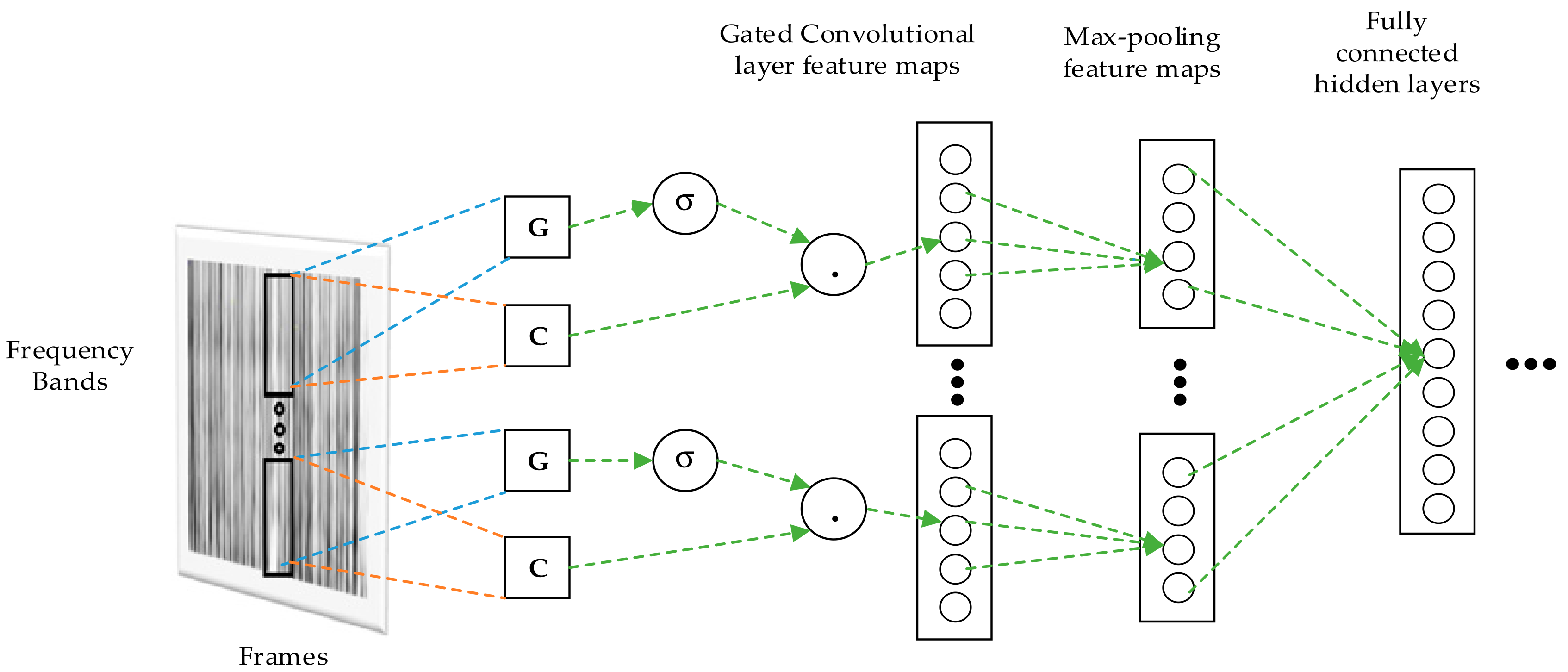
3.1. Gated Convolutional Neural Network Model
3.2. Recurrent Convolutional Neural Network Model
3.3. Gated Recurrent Convolutional Neural Network Model
3.4. Highway Recurrent Convolutional Neural Network Model
3.5. Res-RCNN and Res-RGCNN Models
4. Experimental Results
4.1. Data Corpus
4.2. Results of the Baseline Acoustic Models
4.3. Results of the Proposed Neural Network Models
4.3.1. Gated Convolutional Neural Network Model
4.3.2. Recurrent Convolutional Neural Network Model
4.3.3. Gated Recurrent Convolutional Neural Network Model
4.3.4. Highway Recurrent Convolutional Neural Network Model
4.3.5. Residual Recurrent Convolutional Neural Network Model
4.3.6. Residual Recurrent Gate Convolutional Neural Network Model
4.3.7. Various CNN-BGRU Neural Network Models for All Languages
4.3.8. Training Time, Recognition Speed, and Parameters of the Models
5. Discussion
6. Conclusions and Future Directions
Author Contributions
Funding
Conflicts of Interest
References
- Dahl, G.E.; Yu, D.; Deng, L.; Acero, A. Context-Dependent Pre-Trained Deep Neural Networks for Large Vocabulary Speech Recognition. IEEE Trans. Audio Speech Lang. Process. 2011, 20, 30–42. [Google Scholar] [CrossRef] [Green Version]
- Maas, A.L.; Qi, P.; Xie, Z.; Hannun, A.Y.; Lengerich, C.T.; Jurafsky, D.; Ng, A.Y. Building DNN acoustic models for large vocabulary speech recognition. Comput. Speech Lang. 2017, 41, 195–213. [Google Scholar] [CrossRef] [Green Version]
- Dahl, G.E.; Sainath, T.N.; Hinton, G.E. Improving deep neural networks for LVCSR using rectified linear units and dropout. In Proceedings of the International Conference on Acoustics, Speech and Signal Processing, Vancouver, BC, Canada, 26–31 May 2013; pp. 8609–8613. [Google Scholar]
- Cai, M.; Shi, Y.; Liu, J. Deep maxout neural networks for speech recognition. In Proceedings of the IEEE Workshop on Automatic Speech Recognition and Understanding, Olomouc, Czech Republic, 8–12 December 2013; pp. 291–296. [Google Scholar]
- Zhang, X.; Trmal, J.; Povey, D.; Khudanpur, S. Improving deep neural network acoustic models using generalized maxout networks. In Proceedings of the IEEE International Conference on Acoustics, Speech and Signal Processing, Vancouver, BC, Canada, 26–31 May 2014; pp. 215–219. [Google Scholar]
- Hinton, G.; Deng, L.; Yu, D.; Dahl, G.E.; Mohamed, A.; Jaitly, N.; Senior, A.; Vanhoucke, V.; Nguyen, P.; Sainath, T.N.; et al. Deep Neural Networks for Acoustic Modeling in Speech Recognition: The Shared Views of Four Research Groups. IEEE Signal Process. Mag. 2012, 29, 82–97. [Google Scholar] [CrossRef]
- Fantaye, T.G.; Yu, J.; Hailu, T.T. Investigation of Various Hybrid Acoustic Modeling Units via a Multitask Learning and Deep Neural Network Technique for LVCSR of the Low-Resource Language, Amharic. IEEE Access 2019, 7, 105593–105608. [Google Scholar] [CrossRef]
- Sriranjani, R.; MuraliKarthick, B.; Umesh, S. Investigation of different acoustic modeling techniques for low resource Indian language data. In Proceedings of the Twenty First National Conference on Communications (NCC), Mumbai, India, 27 February–1 March 2015; pp. 1–5. [Google Scholar]
- Sainath, T.N.; Kingsbury, B.; Saon, G.; Soltau, H.; Mohamed, A.; Dahl, G.E.; Ramabhadran, B. Deep Convolutional Neural Networks for Large-scale Speech Tasks. Neural Netw. 2015, 64, 39–48. [Google Scholar] [CrossRef] [PubMed]
- Abdel-Hamid, O.; Mohamed, A.; Jiang, H.; Deng, L.; Penn, G.; Yu, D. Convolutional Neural Networks for Speech Recognition. IEEE/ACM Trans. Audio Speech Lang. Process. 2014, 22, 1533–1545. [Google Scholar] [CrossRef] [Green Version]
- Marryam, M.; Sharif, M.; Yasmin, M.A.; Ahmad, T. Facial expression detection using Six Facial Expressions Hexagon (SFEH) model. In Proceedings of the 2019 IEEE 9th Annual Computing and Communication Workshop and Conference (CCWC), Las Vegas, NV, USA, 7–9 January 2019; pp. 0190–0195. [Google Scholar]
- Cai, M.; Liu, J. Maxout neurons for deep convolutional and LSTM neural networks in speech recognition. Speech Commun. 2016, 77, 53–64. [Google Scholar] [CrossRef]
- Huang, J.; Li, J.; Gong, Y. An analysis of convolutional neural networks for speech recognition. In Proceedings of the IEEE International Conference on Acoustics, Speech and Signal Processing, Brisbane, QLD, Australia, 19–24 April 2014; pp. 4989–4993. [Google Scholar]
- Cai, M.; Shi, Y.; Kang, J.; Liu, J.; Su, T. Convolutional maxout neural networks for low-resource speech recognition. In Proceedings of the 9th International Symposium on Chinese Spoken Language Processing, Singapore, 12–14 September 2014; pp. 133–137. [Google Scholar]
- Sainath, T.N.; Mohamed, A.; Kingsbury, B.; Ramabhadran, B. Deep convolutional neural networks for LVCSR. In Proceedings of the IEEE International Conference on Acoustics, Speech and Signal Processing, Vancouver, BC, Canada, 26–31 May 2013; pp. 8614–8618. [Google Scholar]
- Chan, W.; Lane, I. Deep convolutional neural networks for acoustic modeling in low resource languages. In Proceedings of the IEEE International Conference on Acoustics, Speech and Signal Processing, Queensland, Australia, 19–24 April 2015; pp. 2056–2060. [Google Scholar]
- Saon, G.; Soltau, H.; Emami, A.; Picheny, M. Unfolded recurrent neural networks for speech recognition. In Proceedings of the INTERSPEECH, Singapore, 14–18 September 2014; pp. 343–347. [Google Scholar]
- Alan, G.; Abdelrahman, M.; Geoffrey, H. Speech recognition with deep recurrent neural networks. In Proceedings of the IEEE International Conference on Acoustics, Speech and Signal Processing, Vancouver, BC, Canada, 26–31 May 2013; pp. 6645–6649. [Google Scholar]
- Alan, G.; Navdeep, J.; Abdelrahman, M. Hybrid speech recognition with deep bidirectional lstm. In Proceedings of the IEEE Workshop on Automatic Speech Recognition and Understanding, Olomouc, Czech Republic, 8–12 December 2013; pp. 273–278. [Google Scholar]
- Kang, J.; Zhang, W.; Liu, W.; Liu, J.; Johnson, M.T. Advanced recurrent network-based hybrid acoustic models for low resource speech recognition. Eurasip J. Audio Spee. 2018, 2018, 1–15. [Google Scholar] [CrossRef]
- Chan, W.; Lane, I. Deep Recurrent Neural Networks for Acoustic Modelling. arXiv preprint 2015, arXiv:1504.01482. [Google Scholar]
- Sak, H.; Senior, A.; Beaufays, F. Long short-term memory recurrent neural network architectures for large-scale acoustic modeling. In Proceedings of the INTERSPEECH, Singapore, 14–18 September 2014; pp. 338–342. [Google Scholar]
- Kyunghyun, C.; Bart, V.M.; Caglar, G.; Dzmitry, B.; Fethi, B.; Holger, S.; Yoshua, B. Learning phrase representations using rnn encoder-decoder for statistical machine translation. arXiv preprint 2014, arXiv:1406.1078. [Google Scholar]
- Ravanelli, M.; Brakel, P.; Omologo, M.; Bengio, Y. Light Gated Recurrent Units for Speech Recognition. IEEE Trans. Emerg. Top. Comput. Intell. 2018, 2, 92–102. [Google Scholar] [CrossRef] [Green Version]
- Ravanelli, M.; Brakel, P.; Omologo, M.; Bengio, Y. Improving speech recognition by revising gated recurrent units. In Proceedings of the INTERSPEECH, Stockholm, Sweden, 20–24 August 2017. [Google Scholar]
- Chung, J.; Gulcehre, C.; Cho, K.; Bengio, Y. Empirical evaluation of gated recurrent neural networks on sequence modeling. arXiv 2014, arXiv:1412.3555. [Google Scholar]
- Kang, J.; Zhang, W.; Liu, J. Gated convolutional networks based hybrid acoustic models for low resource speech recognition. In Proceedings of the IEEE Automatic Speech Recognition and Understanding Workshop, Okinawa, Japan, 16–20 December 2017; pp. 157–164. [Google Scholar]
- Nußbaum-Thom, M.; Cui, J.; Ramabhadran, B.; Goel, V. Acoustic Modeling Using Bidirectional Gated Recurrent Convolutional Units. In Proceedings of the INTERSPEECH, San Francisco, CA, USA, 8–12 September 2016; pp. 390–394. [Google Scholar]
- Lu, L.; Renals, S. Small-Footprint Highway Deep Neural Networks for Speech Recognition. IEEE/ACM Trans. Audio Speech Lang. Process. 2017, 25, 1502–1511. [Google Scholar] [CrossRef]
- Pundak, G.; Sainath, T.N. Highway LSTM and Recurrent Highway Networks for Speech Recognition. In Proceedings of the INTERSPEECH, Stockholm, Sweden, 20–24 August 2017; pp. 1303–1307. [Google Scholar]
- Zhou, S.; Zhao, Y.; Xu, S.; Xu, B. Multilingual Recurrent Neural Networks with Residual Learning for Low-Resource Speech Recognition. In Proceedings of the INTERSPEECH, Stockholm, Sweden, 20–24 August 2017; pp. 704–708. [Google Scholar]
- Wang, Y.; Deng, X.; Pu, S.; Huang, Z. Residual Convolutional CTC Networks for Automatic Speech Recognition. arXiv 2017, arXiv:1702.07793. [Google Scholar]
- Tan, T.; Qian, Y.; Hu, H.; Zhou, Y.; Ding, W.; Yu, K. Adaptive Very Deep Convolutional Residual Network for Noise Robust Speech Recognition. IEEE/ACM Trans. Audio Speech Lang. Process. 2018, 26, 1393–1405. [Google Scholar] [CrossRef]
- Sercu, T.; Puhrsch, C.; Kingsbury, B.; LeCun, Y. Very deep multilingual convolutional neural networks for LVCSR. In Proceedings of the IEEE International Conference on Acoustics, Speech and Signal Processing, Shanghai, China, 20–25 March 2016; pp. 4955–4959. [Google Scholar]
- Deng, L.; Platt, J.C. Ensemble Deep Learning for Speech Recognition. In Proceedings of the Interspeech, Singapore, 14–18 September 2014. [Google Scholar]
- Sainath, T.N.; Vinyals, O.; Senior, A.; Sak, H. Convolutional, Long Short-Term Memory, fully connected Deep Neural Networks. In Proceedings of the IEEE International Conference on Acoustics, Speech and Signal Processing, Brisbane, QLD, Australia, 19–24 April 2015; pp. 4580–4584. [Google Scholar]
- Hsu, W.; Zhang, Y.; Lee, A.; Glass, J. Exploiting Depth and Highway Connections in Convolutional Recurrent Deep Neural Networks for Speech Recognition. In Proceedings of the INTERSPEECH, San Francisco, CA, USA, 8–12 September 2016; pp. 395–399. [Google Scholar]
- Wang, D.; Lv, S.; Wang, X.; Lin, X. Gated Convolutional LSTM for Speech Commands Recognition. In Proceedings of the International Conference on Computational Science, Wuxi, China, 11–13 June 2018; pp. 669–681. [Google Scholar]
- Zhao, Y.; Jin, X.; Hu, X. Recurrent convolutional neural network for speech processing. In Proceedings of the IEEE International Conference on Acoustics, Speech and Signal Processing, New Orleans, LA, USA, 5–9 March 2017; pp. 5300–5304. [Google Scholar]
- Tran, D.T.; Delcroix, M.; Karita, S.; Hentschel, M.; Ogawa, A.; Nakatani, T. Unfolded Deep Recurrent Convolutional Neural Network with Jump Ahead Connections for Acoustic Modeling. In Proceedings of the INTERSPEECH, Stockholm, Sweden, 20–24 August 2017; pp. 1596–1600. [Google Scholar]
- Sainath, T.N.; Parada, C. Convolutional neural networks for small-footprint keyword spotting. In Proceedings of the INTERSPEECH, Dresden, Germany, 6–10 September 2015; pp. 1478–1482. [Google Scholar]
- Fantaye, T.G.; Yu, J.; Hailu, T.T. Investigation of Automatic Speech Recognition Systems via the Multilingual Deep Neural Network Modeling Methods for a Very Low-Resource Language, Chaha. J. Signal Inf. Process. 2020, 11, 1–21. [Google Scholar] [CrossRef] [Green Version]
- Fantaye, T.G.; Yu, J.; Hailu, T.T. Syllable-based Speech Recognition for a Very Low-Resource Language, Chaha. In Proceedings of the 2019 2nd International Conference on Algorithms, Computing and Artificial Intelligence (ACAI 2019), Sanya, China, 20–22 December 2019; pp. 415–420. [Google Scholar]
- Pipiras, L.; Maskeliūnas, R.; Damaševičius, R. Lithuanian Speech Recognition Using Purely Phonetic Deep Learning. Computers 2019, 8, 76. [Google Scholar] [CrossRef] [Green Version]
- Rosenberg, A.; Audhkhasi, K.; Sethy, A.; Ramabhadran, B.; Picheny, M. End-to-end speech recognition and keyword search on low-resource languages. In Proceedings of the IEEE International Conference on Acoustics, Speech and Signal Processing, New Orleans, LA, USA, 5–9 March 2017; pp. 5280–5284. [Google Scholar]
- Daneshvar, M.B.; Veisi, H. Persian phoneme recognition using long short-term memory neural network. In Proceedings of the Eighth International Conference on Information and Knowledge Technology (IKT), Hamedan, Iran, 7–8 September 2016; pp. 111–115. [Google Scholar]
- Gales, M.J.F.; Kate, K.; Anton, R. Unicode-based graphemic systems for limited resource languages. In Proceedings of the IEEE International Conference on Acoustics, Speech and Signal Processing, Brisbane, QLD, Australia, 19–24 April 2015; pp. 5186–5190. [Google Scholar]
- Dalen, R.C.; Yang, J.; Wang, H.; Ragni, A.; Zhang, C.; Gales, M.J. Structured discriminative models using deep neural network features. In Proceedings of the IEEE Workshop on Automatic Speech Recognition and Understanding, Scottsdale, Maricopa, AZ, USA, 13–17 December 2015; pp. 160–166. [Google Scholar]
- Bluche, T.; Messina, R. Gated Convolutional Recurrent Neural Networks for Multilingual Handwriting Recognition. In Proceedings of the 14th IAPR International Conference on Document Analysis and Recognition, Kyoto, Japan, 9–15 November 2017; pp. 646–651. [Google Scholar]
- Liu, Y.; Ji, L.; Huang, R.; Ming, T.; Gao, C.; Zhang, J. An Attention Gated Convolutional Neural Network for Sentence Classification. Intell. Data Anal. 2019, 23, 1091–1107. [Google Scholar] [CrossRef] [Green Version]
- Dauphin, Y.N.; Fan, A.; Auli, M.; Grangier, D. Language Modeling with Gated Convolutional Networks. arXiv 2016, arXiv:1612.08083. [Google Scholar]
- Spoerer, C.J.; McClure, P.; Kriegeskorte, N. Recurrent Convolutional Neural Networks: A Better Model of Biological Object Recognition. Front. Psychol. 2017, 8, 1551. [Google Scholar] [CrossRef]
- Lai, S.; Xu, L.; Liu, K.; Zhao, J. Recurrent Convolutional Neural Networks for Text Classification. In Proceedings of the Twenty Ninth AAAI Conference on Artificial Intelligence, Austin, TX, USA, 25–30 January 2015; pp. 2267–2273. [Google Scholar]
- Liang, M.; Hu, X. Recurrent convolutional neural network for object recognition. In Proceedings of the IEEE Conference on Computer Vision and Pattern Recognition, Boston, MA, USA, 7–12 June 2015; pp. 3367–3375. [Google Scholar]
- Liang, M.; Hu, X.; Zhang, B. Convolutional Neural Networks with Intra-Layer Recurrent Connections for Scene Labeling. In Proceedings of the 28th International Conference on Neural Information Processing Systems, Montreal, QC, Canada, 8–13 December 2014; pp. 937–945. [Google Scholar]
- Srivastava, R.K.; Greff, K.; Schmidhuber, J. Highway Networks. arXiv 2015, arXiv:1505.00387. [Google Scholar]
- Bi, M.; Qian, Y.; Yu, K. Very deep convolutional neural networks for LVCSR. In Proceedings of the INTERSPEECH, Dresden, Germany, 6–10 September 2015; pp. 3259–3263. [Google Scholar]
- Lucy, A.; Aric, B.; Thomas, C.; Luanne, D.; Eyal, D.; Jonathan, G.; Mary, H.; Hanh, L.; Arlene, M.; Jennifer, M.; et al. IARPA Babel Cebuano Language Pack IARPA-babel301b-v2.0b LDC2018S07; Web Download; Linguistic Data Consortium: Philadelphia, PA, USA, 2018. [Google Scholar]
- Aric, B.; Thomas, C.; Anne, D.; Eyal, D.; Jonathan, G.; Mary, H.; Brook, H.; Kirill, K.; Jennifer, M.; Jessica, R.; et al. IARPA Babel Kazakh Language Pack IARPA-babel302b-v1.0a LDC2018S13; Web Download; Linguistic Data Consortium: Philadelphia, PA, USA, 2018. [Google Scholar]
- Aric, B.; Thomas, C.; Anne, D.; Eyal, D.; Jonathan, G.F.; Simon, H.; Mary, H.; Alice, K.-S.; Jennifer, M.; Shelley, P.; et al. IARPA Babel Telugu Language Pack IARPA-babel303b-v1.0a LDC2018S16; Web Download; Linguistic Data Consortium: Philadelphia, PA, USA, 2018. [Google Scholar]
- Aric, B.; Thomas, C.; Miriam, C.; Eyal, D.; Jonathan, G.F.; Mary, H.; Melanie, H.; Kirill, K.; Nicolas, M.; Jennifer, M.; et al. IARPA Babel Tok-Pisin Language Pack IARPA-babel207b-v1.0e LDC2018S02; Web Download; Linguistic Data Consortium: Philadelphia, PA, USA, 2018. [Google Scholar]
- Stolcke, A. SRILM-an extensible language modeling toolkit. In Proceedings of the ICSLP, Denver, CO, USA, 16–20 September 2002; pp. 901–904. [Google Scholar]
- Povey, D.; Ghoshal, A.; Boulianne, G.; Burget, L.; Glembek, O.; Goel, N.; Hannemann, M.; Motl´ıcek, P.; Qian, Y.; Schwarz, P.; et al. The Kaldi Speech Recognition Toolkit. In Proceedings of the IEEE ASRU, Waikoloa, HI, USA, 11–15 December 2011. [Google Scholar]
- Ravanelli, M.; Parcollet, T.; Bengio, Y. The PyTorch-Kaldi Speech Recognition Toolkit. In Proceedings of the IEEE International Conference on Acoustics, Speech and Signal Processing, Brighton, UK, 12–17 May 2019; pp. 6465–6469. [Google Scholar]
- Yi, J.; Jianhua, T.; Zhengqi, W.; Ye, B. Adversarial Multilingual Training for Low-Resource Speech Recognition. In Proceedings of the IEEE International Conference on Acoustics, Speech and Signal Processing, Calgary, AB, Canada, 15–20 April 2018; pp. 4899–4903. [Google Scholar]


| Remark | Language | Training Dataset Size (Hours) | Studies | Word Error Rate (WER) (%) | ||||||
|---|---|---|---|---|---|---|---|---|---|---|
| DNN | CNN/Very Deep CNN | TDNN | RNN | LSTM | GRU | End-to-End | ||||
| Ethiopic languages | Chaha | 8.01 | [42] | 23.50 | ||||||
| [43] | 28.05 | |||||||||
| Own | 23.70 | 22.75 | 25.82 | 22.36 | ||||||
| Amharic | 26 | [7] | 11.28 | |||||||
| Own | 11.35 | 10.30 | 12.76 | 9.89 | ||||||
| European Union language | Lithuanian | 52 | [44] | 1.303 | ||||||
| Babel option period three languages | Cebuano | 10.37 | [34] | 76.3 | 74.2/70.3 | |||||
| Own | 68.33 | 67.23 | 72.63 | 66.41 | ||||||
| Kazakh | 39.6 | [20] | 54.1 | 52.9 | ||||||
| 9.92 | [34] | 77.3 | 75.2/71.1 | |||||||
| [47] | 76.2 | |||||||||
| Own | 70.75 | 70.08 | 74.85 | 69.38 | ||||||
| Telugu | 10.21 | [34] | 87.00 | 85.4/82.5 | ||||||
| Own | 86.20 | 86.37 | 89.7 | 84.98 | ||||||
| Tok-Pisin | 9.83 | [34] | 62.6 | 59.4/54.2 | ||||||
| [48] | 52.7 | |||||||||
| Own | 50.14 | 49.35 | 54.71 | 48.22 | ||||||
| Swahili | 44 | [20] | 46.2 | 42.5 | ||||||
| [27] | 42.9 | 42.4 | 42.1 | |||||||
| Indian Languages | Tamil | 22 | [8] | 20.01 | ||||||
| Hindi | 22 | [8] | 3.91 | |||||||
| Babel option period one languages | Bengali | 10 | [16] | 70.8 | 69.2 | |||||
| Cantonese | 140.7 | [12] | 44.8 | 46.1 | 40.7 | |||||
| Pashto | 77.3 | 51.2 | 52.0 | 50.5 | ||||||
| [20] | 51.2 | 50.5 | ||||||||
| Turkish | 76.3 | [12] | 47.6 | 47.6 | 47.4 | |||||
| Tagalog | 83.7 | 49.8 | 49.6 | 47.9 | ||||||
| Vietnamese | 87.1 | 53.1 | 51.8 | 47.8 | ||||||
| [20] | 53.1 | 47.8 | ||||||||
| Tamil | 62.3 | [12] | 66.7 | 66.0 | 65.0 | |||||
| [20] | 66.7 | 65.0 | ||||||||
| Iranian language | Persian | 15 | [46] | 21.86 | 17.55 | |||||
| Model | GCNN | RCNN | Res-RCNN |
|---|---|---|---|
| Input map size | 11 × 40 Filterbank | 11 × 40 Filterbank | 11 × 40 Filterbank |
| # layers | 3 GCLs | 3 RCLs | 3 Res-RCLs |
| 60 feature maps | GRCL (3, 60) Max pooling (3) Layer-Normalization ReLU Dropout (0.15) | RCL (3, 60) Max pooling (3) Layer-Normalization ReLU Dropout (0.15) | Res-RCL (3, 60) Max pooling (3) Layer-Normalization ReLU Dropout (0.15) |
| 60 feature maps | GRCL (3, 60) Max pooling (2) Layer-normalization ReLU Dropout (0.15) | RCL (3, 60) Max pooling (2) Layer-normalization ReLU Dropout (0.15) | Res-RCL (3, 60) Max pooling (2) Layer-normalization ReLU Dropout (0.15) |
| 60 feature maps | GRCL (3, 60) Layer-Normalization ReLU Dropout (0.15) | RCL (3, 60) Layer-Normalization ReLU Dropout (0.15) | Res-RCL (3, 60) Layer-Normalization ReLU Dropout (0.15) |
| 4 Fully connected layers (1024 nodes, batch-normalization, dropout (0.15)) or 3 BGRU layers (550 nodes, batch-normalization, dropout (0.2)) | |||
| Softmax output layer | |||
| Model | CNN | GRCNN | HRCNN | Res-RGCNN |
|---|---|---|---|---|
| Input map size | 11 × 40 Filterbank | 11 × 40 Filterbank | 11 × 40 Filterbank | 11 × 40 Filterbank |
| # layers | 2 conv. layers | 3 GRCLs | 3 HRCLs | 3 Res-RGCLs |
| 80 feature maps | conv. (3, 80) Max pooling (3) Layer-normalization ReLU Dropout(0.15) | GRCL (3, 80) Max pooling (3) Layer-normalization ReLU Dropout (0.15) | HRCL (3, 80) Max pooling (3) Layer-normalization ReLU Dropout (0.15) | Res-RGCL (3, 80) Max pooling (3) Layer-normalization ReLU Dropout (0.15) |
| 80 feature maps | Conv. (3, 80) Layer-normalization ReLU Dropout(0.15) | GRCL (3, 80) Max pooling (2) Layer-normalization ReLU Dropout (0.15) | HRCL (3, 80) Max pooling (2) Layer-normalization ReLU Dropout (0.15) | Res-RGCL (3, 80) Max pooling (2) Layer-normalization ReLU Dropout (0.15) |
| 80 feature maps | GRCL (3, 80) Layer-normalization ReLU Dropout (0.15) | HRCL (3, 80) Layer-normalization ReLU Dropout (0.15) | Res-RGCL (3, 80) Layer-normalization ReLU Dropout (0.15) | |
| 4 Fully connected layers (1024 nodes, batch-normalization, dropout (0.15)) or 3 BGRU layers (550 nodes, batch-normalization, dropout (0.2)) | ||||
| Softmax output layer | ||||
| Language | ID | Release | Description |
|---|---|---|---|
| Cantonese | 101 | IARPA-babel101-v0.4c | Babel option period one languages |
| Pashto | 104 | IARPA-babel104b-v0.4aY | |
| Tagalog | 106 | IARPA-babel106-v0.2g | |
| Vietnamese | 107 | IARPA-babel107b-v0.7 | |
| Assamese | 102 | IARPA-babel102b-v0.5a | Babel option period two languages |
| Bengali | 103 | IARPA-babel103b-v0.4b | |
| Haitian Creole | 201 | IARPA-babel201b-v0.2b | |
| Lao | 203 | IARPA-babel203b-v3.1a | |
| Tamil | 204 | IARPA-babel204b-v1.1b | |
| Zulu | 206 | IARPA-babel206b-v0.1e | |
| Swahili | 202 | IARPA-babel202b-v1.0d | Babel option period three languages |
| Kurdish | 205 | IARPA-babel205b-v1.0a | |
| Tok-Pisin | 207 | IARPA-babel207b-v1.0c | |
| Cebuano | 301 | IARPA-babel301b-v2.0b | |
| Kazakh | 302 | IARPA-babel302b-v1.0a | |
| Telugu | 303 | IARPA-babel303b-v1.0a | |
| Lithuanian | 304 | IARPA-babel304b-v1.0b | |
| Guarani | 305 | IARPA-babel305b-v1.0b | Babel option period four languages |
| Igbo | 306 | IARPA-babel306b-v2.0c | |
| Amharic | 307 | IARPA-babel307b-v1.0b | |
| Mongolian | 401 | IARPA-babel401b-v2.0b | |
| Javanese | 402 | IARPA-babel402b-v1.0b | |
| Dholuo | 403 | IARPA-babel403b-v1.0b |
| Language | Training Dataset | Development Dataset | ||||
|---|---|---|---|---|---|---|
| # of Speaker | # of Sentences | Duration (Hours) | # of Speakers | # of Sentences | Duration (Hours) | |
| Amharic | 125 | 13,549 | 26.00 | 20 | 359 | 1.00 |
| Chaha | 15 | 5334 | 8.01 | 5 | 222 | 0.33 |
| Cebuano | 127 | 11,215 | 10.37 | 134 | 11,199 | 10.27 |
| Kazakh | 130 | 11,570 | 9.92 | 140 | 11,678 | 9.73 |
| Telugu | 134 | 11,150 | 10.21 | 120 | 10,120 | 9.74 |
| Tok-Pisin | 127 | 9820 | 9.83 | 132 | 10,156 | 9.92 |
| Language | Lexicon Size (Number of Words) | Number of Phonemes | Language Model Perplexity |
|---|---|---|---|
| Amharic | 85,000 | 233 | 76 |
| Chaha | 4000 | 41 | 103 |
| Cebuano | 7617 | 28 | 129 |
| Kazakh | 8552 | 61 | 229 |
| Telugu | 15,552 | 50 | 461 |
| Tok-Pisin | 3780 | 37 | 77 |
| Model | WER (%) | |||||
|---|---|---|---|---|---|---|
| Amharic | Chaha | Cebuano | Kazakh | Telugu | Tok-Pisin | |
| DNN | 11.35 | 23.70 | 68.33 | 70.75 | 86.20 | 50.14 |
| CNN | 10.30 | 22.75 | 67.23 | 70.08 | 86.37 | 49.35 |
| BRNN | 12.76 | 25.82 | 72.63 | 74.85 | 89.70 | 54.71 |
| BGRU | 9.89 | 22.36 | 66.41 | 69.38 | 84.98 | 48.22 |
| Remark | Model | WER (%) | |||||
|---|---|---|---|---|---|---|---|
| Amharic | Chaha | Cebuano | Kazakh | Telugu | Tok-Pisin | ||
| Baseline neural network models | DNN | 11.35 | 23.70 | 68.33 | 70.75 | 86.20 | 50.14 |
| CNN | 10.30 | 22.75 | 67.23 | 70.08 | 86.37 | 49.35 | |
| BRNN | 12.76 | 25.82 | 72.63 | 74.85 | 89.7 | 54.71 | |
| BGRU | 9.89 | 22.36 | 66.41 | 69.38 | 84.98 | 48.22 | |
| Proposed neural network models | GCNN | 9.95 | 22.35 | 67.08 | 70.01 | 86.02 | 48.99 |
| RCNN | 9.63 | 22.05 | 66.66 | 69.27 | 85.62 | 48.45 | |
| GRCNN | 9.73 | 22.11 | 66.63 | 69.29 | 85.40 | 48.49 | |
| HRCNN | 9.83 | 22.19 | 66.58 | 69.25 | 85.33 | 48.58 | |
| Res-RCNN | 9.66 | 22.02 | 66.64 | 69.27 | 85.55 | 48.44 | |
| Res-RGCNN | 9.58 | 21.93 | 66.49 | 69.17 | 85.25 | 48.37 | |
| CNN-BGRU | 9.35 | 21.69 | 66.33 | 69.28 | 84.94 | 48.15 | |
| GCNN-BGRU | 8.85 | 21.14 | 66.03 | 69.08 | 84.18 | 47.39 | |
| RCNN-BGRU | 8.20 | 20.38 | 65.35 | 67.57 | 83.33 | 46.25 | |
| GRCNN-BGRU | 8.00 | 20.15 | 65.26 | 67.53 | 82.77 | 46.23 | |
| HRCNN-BGRU | 7.85 | 19.97 | 65.11 | 67.39 | 82.85 | 46.18 | |
| Residual RCNN-BGRU | 7.92 | 20.05 | 65.33 | 67.51 | 83.30 | 46.23 | |
| Residual RGCNN-BGRU | 7.30 | 19.78 | 65.00 | 67.25 | 82.90 | 45.95 | |
| Best case absolute WER (%) reduction | 5.46 | 6.04 | 7.63 | 7.6 | 6.8 | 8.76 | |
| Time-Steps | WER (%) |
|---|---|
| 1 | 48.46 |
| 2 | 48.45 |
| 3 | 48.48 |
| Remark | Model | Training Time per Epoch (Hours) | Average RTF per Model | Model Size | |||||
|---|---|---|---|---|---|---|---|---|---|
| Am. | Ch. | Ceb. | Ka. | Tel. | Tok. | ||||
| Baseline neural network models | DNN | 0.25 | 0.09 | 0.11 | 0.15 | 0.17 | 0.16 | 9.788 | 7.7 |
| CNN | 0.70 | 0.33 | 0.37 | 0.35 | 0.39 | 0.38 | 7.651 | 13.9 | |
| BRNN | 0.38 | 0.17 | 0.20 | 0.19 | 0.22 | 0.21 | 11.814 | 2.2 | |
| BGRU | 1.12 | 0.54 | 0.61 | 0.56 | 0.63 | 0.59 | 9.756 | 8.7 | |
| Proposed neural network models | GCNN | 0.5 | 0.23 | 0.25 | 0.27 | 0.29 | 0.28 | 8.113 | 19.8 |
| RCNN | 1.40 | 0.66 | 0.69 | 0.70 | 0.73 | 0.71 | 7.865 | 19.8 | |
| GRCNN | 2.90 | 1.30 | 1.45 | 1.46 | 1.48 | 1.45 | 8.143 | 24.8 | |
| HRCNN | 3.04 | 1.50 | 1.53 | 1.55 | 1.54 | 1.52 | 8.8599 | 24.8 | |
| Res-RCNN | 1.38 | 0.67 | 0.69 | 0.73 | 0.70 | 0.71 | 7.865 | 19.8 | |
| Res-RGCNN | 3.08 | 1.52 | 1.55 | 1.56 | 1.58 | 1.54 | 8.8745 | 25.9 | |
| CNN-BGRU | 1.82 | 0.88 | 0.98 | 0.91 | 1.02 | 0.97 | 7.764 | 23.9 | |
| GCNN-BGRU | 1.73 | 0.82 | 0.86 | 0.87 | 0.92 | 0.87 | 8.342 | 28 | |
| RCNN-BGRU | 2.55 | 1.22 | 1.30 | 1.26 | 1.36 | 1.30 | 7.849 | 28 | |
| GRCNN-BGRU | 4.08 | 2.00 | 2.14 | 2.10 | 2.11 | 2.04 | 8.523 | 34.5 | |
| HRCNN-BGRU | 2.22 | 2.08 | 2.14 | 2.11 | 2.17 | 2.11 | 8.872 | 34.6 | |
| Residual RCNN-BGRU | 2.60 | 1.27 | 1.30 | 1.29 | 1.33 | 1.30 | 7.912 | 28 | |
| Residual RGCNN-BGRU | 4.40 | 2.09 | 2.16 | 2.12 | 2.21 | 2.13 | 8.976 | 36.6 | |
© 2020 by the authors. Licensee MDPI, Basel, Switzerland. This article is an open access article distributed under the terms and conditions of the Creative Commons Attribution (CC BY) license (http://creativecommons.org/licenses/by/4.0/).
Share and Cite
Fantaye, T.G.; Yu, J.; Hailu, T.T. Advanced Convolutional Neural Network-Based Hybrid Acoustic Models for Low-Resource Speech Recognition. Computers 2020, 9, 36. https://doi.org/10.3390/computers9020036
Fantaye TG, Yu J, Hailu TT. Advanced Convolutional Neural Network-Based Hybrid Acoustic Models for Low-Resource Speech Recognition. Computers. 2020; 9(2):36. https://doi.org/10.3390/computers9020036
Chicago/Turabian StyleFantaye, Tessfu Geteye, Junqing Yu, and Tulu Tilahun Hailu. 2020. "Advanced Convolutional Neural Network-Based Hybrid Acoustic Models for Low-Resource Speech Recognition" Computers 9, no. 2: 36. https://doi.org/10.3390/computers9020036