Abstract
Free riding incentives make it difficult to control climate change. To improve the chances of the Paris Agreement’s ambitious goal, many nations are forming scientific networks in carbon capture and storage (CCS). These networks take many forms (bilateral, hub-and-spoke, and multilateral). Studies of social interactions among scientists demonstrate that research networks are limited because of relational issues, such as lack of trust. This paper provides a rationale for the formation of various types of international CCS networks and examines their impacts on climate change. Our concept of stability focuses on Nash equilibria that are immune to coalitional deviations in overlapping networks. Players may belong to various research networks. A particular research network is a climate club. We show that in the absence of top-down coordination in clubs, the type of global network that forms depends on relational attrition. The complex task is to mitigate free riding while enhancing trust.
1. Introduction
On 2 November 2021, during the Conference of Parties (COP26) in Glasgow, the prime minister of Canada, Justin Trudeau, pushed the world to commit to a global carbon tax by 2030 that will account for 60% of global greenhouse emissions (see https://www.ctvnews.ca/politics/trudeau-takes-carbon-pricing-debate-to-the-global-stage-at-cop26-1.5648007; accessed on 18 October 2021). This challenge signals a widespread concern about the catastrophic effects that unabated global warming will cause to all nations in the near future. Voluntary national commitments made under the Paris Agreement (PA) may be insufficient to deliver the desirable goal of preventing an increase of more than 2 degrees Celsius in global temperature by the end of the century. A global carbon tax may be ideal, but it may be politically and institutionally difficult to design and implement. One should consider more realistic alternatives.
Among possible alternatives to a global carbon tax, one that is especially noteworthy is the creation of climate clubs. Nordhaus [1] proposes the formation of climate clubs to overcome free riding in climate policy. Clubs motivate participation by providing an excludable public good (club good). Only club members enjoy the benefits associated with the provision of the club good. In Nordhaus [1], the club good is a common carbon tax that all members agree to impose on activities that cause carbon emissions. As the common carbon tax promotes outside benefits to non-club members, the club mechanism also punishes non-club members through trade sanctions.
In this paper, we build on the notion proposed by Nordhaus but focus on another type of club good: R&D spillovers shared by club members produced by improvements in carbon abatement. We also extend the concept by considering overlapping climate clubs. A member of a club may simultaneously belong to another club. Unlike Nordhaus [1], we examine settings where club formation accounts for unilateral and coalitional deviations, and there is no punishment imposed on players that stand alone (i.e., do not join any club), (see Silva and Kahn [2] for an early analysis of exclusion incentives in voluntary club good provision, in which coalition-proofness is utilized to select a stable Nash equilibrium).
The PA’s ambitious goal of limiting an increase in the global temperature to no more than 2 degrees Celsius by the end of the century can only be achieved by further technological development and a combination of several carbon emission reduction strategies, including carbon capture and storage (CCS) (see e.g., “The Global Status of CCS: 2017”). CCS has tremendous potential to reduce global carbon emissions (see, e.g., de Coninck et al. [3], Herzog [4], Leach et al. [5] and The Royal Society [6]). Not surprising, Australia, Canada, China, the EU, India, Japan, Korea, Norway, South Africa, the UK, and the USA have been active in the formation of international joint CCS agreements. Notably, China and the EU are “hubs” in the CCS network: they are central pieces of multiple bilateral and multilateral international agreements (see, e.g., Hagemann et al. [7]).
The fact that China and the EU have entered into several bilateral and multilateral CCS agreements illustrates a major advantage of such a strategy. A large research network enables China or the EU to have access to new as well as complementary pieces of knowledge and reduces the likelihoods of inertia and redundancy in its R&D process. The amount of R&D spillovers enjoyed by a nation may significantly increase as it forms new partnerships. Several studies find that the size of a research team (i.e., research network size) is positively correlated to various types of indicators of the number and quality of publications (see, e.g., Defazio et al. [8]).
However, there are also important factors that limit the efficient size of research networks. In the case of CCS, the inherent interdependency of the various research tasks (i.e., carbon capture, logistics, and storage) implies that research teams need to be very cohesive. The knowledge underlying CCS projects seem to fit well the description of complex knowledge in Sorenson et al. [9]. Complexity is defined “…in terms of the level of interdependence inherent in the subcomponents of a piece of knowledge…Interdependence arises when a subcomponent significantly affects the contribution of one or more other subcomponents to the functionality of a piece of knowledge. When subcomponents are interdependent, a change in one may require the adjustment, inclusion or replacement of others for a piece of knowledge to remain effective.” (Sorenson et al. [9] (p. 995)). Cohesive research teams are those in which research collaborators are prone to cooperate in knowledge creation and diffusion because they have a great deal of trust in each other (see, e.g., Forti et al. [10]. These authors find that research teams are more productive the more cohesive they are. This finding gives support to the idea that strong ties among research collaborators promote trust and cooperation, and these factors enable these researchers to effectively enhance mutual exchange of highly sensitive and fine-grained information. Their result adds to the controversy of which weak or strong ties among researchers are more important for knowledge creation and diffusion. As hypothesized by Granovetter [11], weak ties among individuals may facilitate bridge formation and information diffusion). Trust among research collaborators builds slowly because collaborators prefer past or existing relationships to new collaborations (see, e.g., Goyal [12], pp. 259–261). The argument is that researchers who contemplate new collaborations face a substantial lack of knowledge with respect to each other’s opportunistic behavior. This creates a moral hazard problem, which may reduce communication and knowledge sharing within the research team.
In this paper, we focus on R&D production that emerges from interactions among research teams across nations. In Fershtman and Gandal [13], direct project spillovers “exist whenever there are knowledge spillovers between projects that are directly connected, that is, they have common contributors” and indirect project spillovers “exist whenever there are knowledge spillovers between projects that are not directly connected, that is, projects for which there are no common contributors.” In our multilateral R&D agreements, there exist direct project spillovers only. In our hub-and-spoke R&D agreements, there are both direct and indirect project spillovers. Fershtman and Gandal [13] find evidence of direct and indirect project spillovers in their analysis of open-source software. We follow the basic premise of the “coauthor model” developed by Jackson and Wollinsky [14] that the benefits of the interaction between a pair of research collaborators are both the benefit that each collaborator puts into the project and the benefit associated with synergy.
As for the costs of joint R&D activities in clubs, we consider the cost of hiring inputs (labor and capital) and the transaction costs that lack of trust produces. Transaction costs generate efficiency losses, measured in terms of the potential R&D product foregone. We account for two potential sources of efficiency losses. First, lack of trust weakens ties between any pair of researcher collaborators due to moral hazard issues. International research collaboration is also more likely to be less efficient than domestic research collaboration because of the extra burden faced by researchers in traveling long distances and dealing with differences in time zones (which affect the proper times for one-on-one communication over the internet) and in culture and social working habits. We call the loss of efficiency due to the weakening of ties between collaborators “relational attrition cost”. Second, the total relational attrition cost faced by any researcher should be proportional to the number of collaborators that this individual possesses since the moral hazard problem becomes more severe as the number of partners expands (for example, in his study of R&D performance carried out in one of the U.S. armed services’ largest R&D stations in the early 1960s, Friedlander [15] found that trust among team members was negatively affected by team size).
Following the bottom-up approach embedded in the Paris Agreement, we initially considered a setting in which there are no income transfers within clubs and research collaboration among club members is not coordinated (i.e., R&D spillovers are not internalized). We started the analysis with three nations. We have several results. We first show that a nation that stands alone in the presence of a bilateral club necessarily enjoys an equilibrium payoff that is lower than the common equilibrium payoff earned by the bilateral club members. Even though the stand-alone nation free rides on the emission reductions produced by the bilateral club members, it does not directly benefit from R&D sharing (i.e., the club good). Second, we show that all possible club structures are Perfectly Coalition-Proof-Nash Equilibria (PCPNE) for different ranges of transaction costs. Third, if climate clubs allow and coordinate ex-post transfers, the transfer mechanisms align the incentives of club members: each member finds it desirable to produce R&D at levels that internalize both types of positive externalities within the club. Fourth, in contrast to the situation without transfers, a nation that stands alone in the presence of a bilateral club now enjoys an equilibrium payoff that is higher than the common equilibrium payoff earned by the bilateral club members. The reason for this is that the benefits from free riding outweigh the benefits produced by R&D sharing. Finally, we obtain significantly different equilibrium payoff rankings and PCPNE for larger economies, depending on whether or not clubs implement income transfers (for a comprehensive analysis of network formation in the presence of transfers, see Bloch and Jackson [16]).
We organize the paper as follows. Section 2 provides a brief review of the literature. Section 3 builds the basic model for an economy featuring three nations. Section 4 determines PCPNE for settings in which R&D agreements prohibit or allow transfers. Section 5 provides an analysis of global welfare. Section 6 examines PCPNE with and without transfers for larger economies. Section 7 offers concluding remarks.
2. Literature Review
Our paper contributes to the vast literature on international environmental agreements (see, e.g., Carraro and Siniscalco [17], Barrett [18], Eyckmans and Tulkens [19], Diamantoudi and Sartzetakis [20,21], Diamantoudi, E., E.S. Sartzetakis, and S. Strantza [22,23], Chander [24], Osmani and Tol [25], Silva and Zhu [26], Battaglini and Harstad [27], Silva [28], Bayramoglu et al. [29], Breton and Sbragia [30] and Finus et al. [31]) and to the literature on environmental R&D (see, e.g., Greaker and Hoel [32] and Golombek and Hoel [33]). With the exception of Finus and Rundshagen [34] and Silva and Zhu [26], the coalition-proof approach we utilize here deviates from the ones utilized in the literature on international environmental agreements. Coalition-proofness is a refinement of Nash equilibrium. As for our key contributions to the literature on environmental R&D, to the best of our knowledge, we are the first ones to model the production of collaborative R&D in overlapping international research networks and, therefore, the first to consider the efficiency and stability of overlapping climate clubs.
CCS agreements provide just one of the motivations behind the emergence of hub-and-spoke networks among nations. Indeed, perhaps, the greatest motivation for the development of such networks is trade expansion (see, e.g., Mukunoki and Tachi [35] and Saggi and Yildiz [36]; for additional references, see these papers and Hur et al. [37]). Mukunoki and Tachi [35] study sequential negotiations of bilateral free trade agreements and show that hub-and-spoke networks are likely to be more effective in delivering multilateral free trade than the alternative system of customs unions. They also show that there is an incentive for a nation to be a hub since the hub nation enjoys greater welfare than the spoke nations in equilibrium. Like Mukunoki and Tachi [35], we show that the hub nation in a hub-and-spoke structure without income transfers fares better than the spoke nations. The “hub-incentive effect” disappears if the climate clubs implement income transfers since club members get the same level of welfare in equilibrium.
3. Basic Model
We follow Silva and Zhu [26], who extend the concept of Perfectly Coalition-Proof-Nash Equilibrium (PCPNE), advanced by Bernheim et al. [38], to settings in which overlapping coalitions may coexist. It employs the PCPNE concept to the sets of players produced by the union of intersecting (i.e., overlapping) sets of players.
Suppose that denotes the set of all players. In addition to , the subsets of the set of all players are the singletons and the pairs ,,. The standard coalition-proof concept is applicable to all coalitional structures except to the overlapping ones, in which one nation is a hub. The extended concept of Silva and Zhu [26] is applicable to the overlapping coalitional structures: it is employed over the union of the overlapping bilateral coalitions; namely, the set . Consider, for example, the coalitional structure in which nation 1 is a hub and nations 2 and 3 are spokes; that is, the coalitions and coexist in equilibrium. The Nash equilibrium for this structure is coalition-proof if and only if there is no individual nor collective incentive to deviate; that is, player 1 has no incentive to exit either coalition, and players 2 and 3 have no incentives to exit their respective coalitions in order to stand alone or to form the bilateral coalition . The latter is one of the possible self-enforcing sub-coalitions that can be produced from the set .
The game considered here is a strategic network formation game. We formulate a multistage game, in which the first stage is a participation stage. If the climate clubs prohibit transfers, the game contains two stages: following the participation stage, there is a contribution stage. If the climate clubs allow transfers, the game also includes a third stage in which clubs implement transfers. Formally, the participation stage can be described as follows: For a game where , a pointing game is a list , where for each (a representative element describes the countries that country is pointing towards to initiate a club, and means that country selects country , while means that country does not select country , and for each . We later extend the model to allow for a larger number of nations. For , where , and multiple clubs , let and for all . The equilibrium concept is PCPNE. Finus and Rundshagen [39] argue that the Strong Nash equilibrium instead of the CPNE is useful for many economic problems belonging to the class of positive externality games such as IEAs. However, it is not the case for R&D collaboration in our setting since each nation collaborates not to maximize aggregate payoffs to the coalition but to maximize its own payoff by decreasing production costs. In this case, there is no Strong Nash equilibrium because the grand coalition structure is not Pareto-optimal.
In the basic model, our economy consists of three identical nations, with each nation being indexed by , . There is one consumer in each nation. The utility consumer gets from consumption of units of a numeraire good and units of a pure public good (say, reduction in global carbon dioxide emissions through CCS technology) is , . The budget constraint for consumer is , where is nation ’s cost of contributing units of R&D utilizing its own resources (i.e., working alone) and is nation ’s total income. We assume that , where is a scale parameter. We also assume that is sufficiently large so that all Nash equilibria examined below are characterized by strictly positive consumption of the numeraire good (these details of our basic model are widely used in the environmental economics literature which examines transboundary pollution issues; see, e.g., Diamantoudi and Sartzetakis [20], Nagase and Silva [40], Silva and Yamaguchi [41], and Silva and Zhu [42].
We assume that one unit of carbon-reducing R&D product reduces one unit of carbon emission. If nation is an independent R&D producer, its contribution to carbon-emission reduction is equal to . If nation collaborates with at least one nation in R&D production, nation ’s contribution to carbon-emission reduction is equal to (in the absence of relational attrition), where denotes the total spillover R&D flow that enjoys from its collaborators. We follow previous works on cooperative R&D with spillovers in oligopolies and R&D teams. Nation ’s R&D output increases on its collaborators’ R&D efforts due to knowledge sharing (see, e.g., Spence [43], Katz [44], d’Aspremont and Jacquemin [45], Yi and Shin [46] and Huang [47]) and collaborative problem solving, learning, and feedbacks (see, e.g., Friedlander [15], Dailey [48] and Bruns [49]). We assume that , where denotes the fraction of one unit of time that nation dedicates to itself (i.e., the fraction of time spent alone in research) and to each of its collaborators (i.e., the fraction of time producing synergy in research) when this nation belongs to a research network containing nations (including itself), and is the total R&D effort that ’s collaborators produce. That is, the amount of knowledge spillover that nation receives from each of its collaborators is equal to the product of the fraction of synergistic time it spends with a collaborator and the amount of R&D output produced by a collaborator.
Having discussed the key components of R&D products, let us now turn to the impact of relational attrition on R&D products. Relational attrition reduces the R&D output produced by a nation that is engaged in R&D collaboration. Let denote the relational attrition faced by in its R&D team (possibly composed of partners who belong to multiple clubs). Let be the relational efficiency level experienced by in its R&D team. For simplicity, we assume that . This implies that if and if . Let , where is the rate of relational attrition and denotes the size of ’s R&D team (including self). Formally, the size of ’s R&D team can be defined as follows. Given a nondirected graph , let be the set of ’s collaborators under . Let be the cardinality of R&D team (which includes ). Hence, is the size of ’s R&D team excluding self. This symmetric formulation assumes that faces the same loss in efficiency from relational attrition through its research interactions with any of its R&D collaborators. We have considered different specifications for the efficiency function, for example, , but the qualitative results regarding payoff rankings remain the same. Hence, we chose the specification described above because of its simplicity and its intuitive appeal since ; that is, the marginal efficiency loss associated with increasing a nation’s network size from two to three nations is equal to the attrition rate. As one nation is added to the network with two nations, it makes sense to think that the implied efficiency loss is equal to the additional loss that the extra nation imposes in terms of attrition, namely, a quantity equal to the attrition rate. Then, nation ’s relational efficiency rate works as a scaling function: it transforms nation ’s potential R&D output into nation ’s actual R&D output: . Bruns [49] notes that expert and collaborative practices reinforce each other and are also glued and influenced by the coordination practice that emerges within R&D teams. Hence, we postulate that relational attrition in collaborative practice should affect the entire R&D production process, scaling down the potential R&D output that each researcher can produce (see also Forti et al. [10]). Finally, we assume that the attrition rate is not more than one so that the amount of R&D produced through collaboration is equal to or greater than that by single nations who are standing alone. That is, nation i ’s R&D collaboration is weakly efficient compared to the singleton equilibrium if , where denotes the amount of R&D among singletons. Evaluating the above expression with yields , which is nonnegative as long as . Otherwise, no country will have an incentive to collaborate with other countries.
4. Equilibrium Analysis
The participation stage may produce several club structures depending on the values of the parameters of the model. We need to consider all possible club structures that may result in the participation stage and then compare the equilibrium payoffs in order to determine the PCPNE. We examine two different settings: (i) without transfers within clubs; and (ii) with coordinated transfers within clubs.
4.1. Equilibrium without Transfers
In the participation stage, the possible club structures are:
- (i)
- The singleton structure—all nations are independent (i.e., stand alone);
- (ii)
- The isolated bilateral structure—two nations belong to a club and one nation stands alone;
- (iii)
- The hub-and-spoke structure—one nation forms bilateral clubs with the other two nations (i.e., the hub) and the latter form bilateral clubs with the hub only (i.e., the spokes); and
- (iv)
- The multilateral structure—each nation forms bilateral clubs with the other two nations. In our framework, this is equivalent to the Grand Coalition.
Consider the multilateral structure. In the Nash equilibrium for the contribution game, contributions are determined according to the first-order conditions, , where denotes nation ’s R&D effort, denotes the total amount of the global public good, and represents nation ’s R&D product. The symmetry in interactions implies that all nations earn the same payoff in the Nash equilibrium for the contribution game, , .
In a hub-and-spoke structure, only the hub interacts directly with the other nations (the spokes). Since there is asymmetry in interactions, the Nash equilibrium for the contribution game, the hub earns a higher payoff than the spokes. This important result is gathered in the following lemma:
Lemma 1.
For all, a hub nation’s welfare is higher than a spoke nation’s welfare.
Proof.
Consider the hub-and-spoke structure in which nation 1 is the hub. Let , denote the Nash equilibrium R&D output levels. Let , denote the nations’ own R&D contributions in the Nash equilibrium. The conditions that characterize the Nash equilibrium are
See also Appendix C for the corresponding second-order conditions.
Equation (1b) imply that . Equations (1a) and (1b), the crowding properties of the efficiency function and the strict convexity of the cost function, imply that . To see this, note that is implied by Equations (1a) and (1b). Hence, for all . Since this implies that for all and , we obtain for all . The equilibrium payoff earned by the hub nation is , where . The equilibrium payoff for a spoke nation is . It follows that for all because for all and . □
The hub premium follows from the fact that the hub nation spends fewer resources to produce R&D than the spoke nations when the attrition rate is positive. This result is consistent with the result obtained by Mukunoki and Tachi [35] in that a hub enjoys a premium relative to a spoke, even though the essential details that generate our result are quite different from the essential details that lead to their result. Mukunoki and Tachi [35] examine the free-trade agreements (FTAs) in an oligopoly model. In their model, the abolition of protective tariffs via bilateral FTAs increases the hub’s gains from increasing consumer surplus and the benefits from free access to spoke markets more than the losses from decreases in the profit of the domestic firm and its tariff revenue. Since trade barriers between spoke countries give the hub an advantage in their markets, being a hub is better than having multilateral free trade.
In the isolated bilateral club structure, the stand-alone nation does not enjoy R&D spillovers. The nations that form a bilateral club enjoy R&D spillovers from each other. Thus, in the Nash equilibrium for the contribution game, the equilibrium payoffs for the nations that form a bilateral club are always the same. The following lemma informs us that in the Nash equilibrium for the contribution game, the stand-alone nation is never better off than the nations that form a bilateral club:
Lemma 2.
The equilibrium payoff for the stand-alone nation in the contribution game is never greater than the equilibrium payoffs for the nations that belong to the bilateral club. The stand-alone nation is worse off than the other nations whenever.
Proof.
Consider the isolated bilateral structure in which nations 1 and 2 collaborate and nation 3 stands alone. Let , , denote the Nash equilibrium green R&D product levels. Let , , denote the nations’ own R&D contributions in the Nash equilibrium. The first-order conditions that characterize the Nash equilibrium are
See also Appendix C for the second-order conditions.
The equilibrium payoffs are , , and . Hence, if and only if , . But because . If , and , , and and , , otherwise. □
Let us now determine the PCPNE. Anticipating the Nash equilibria payoffs for the contribution games, each nation decides which clubs it will join, if any, in the network formation stage. To determine the PCPNE, we must compare the Nash equilibria payoffs for the contribution games.
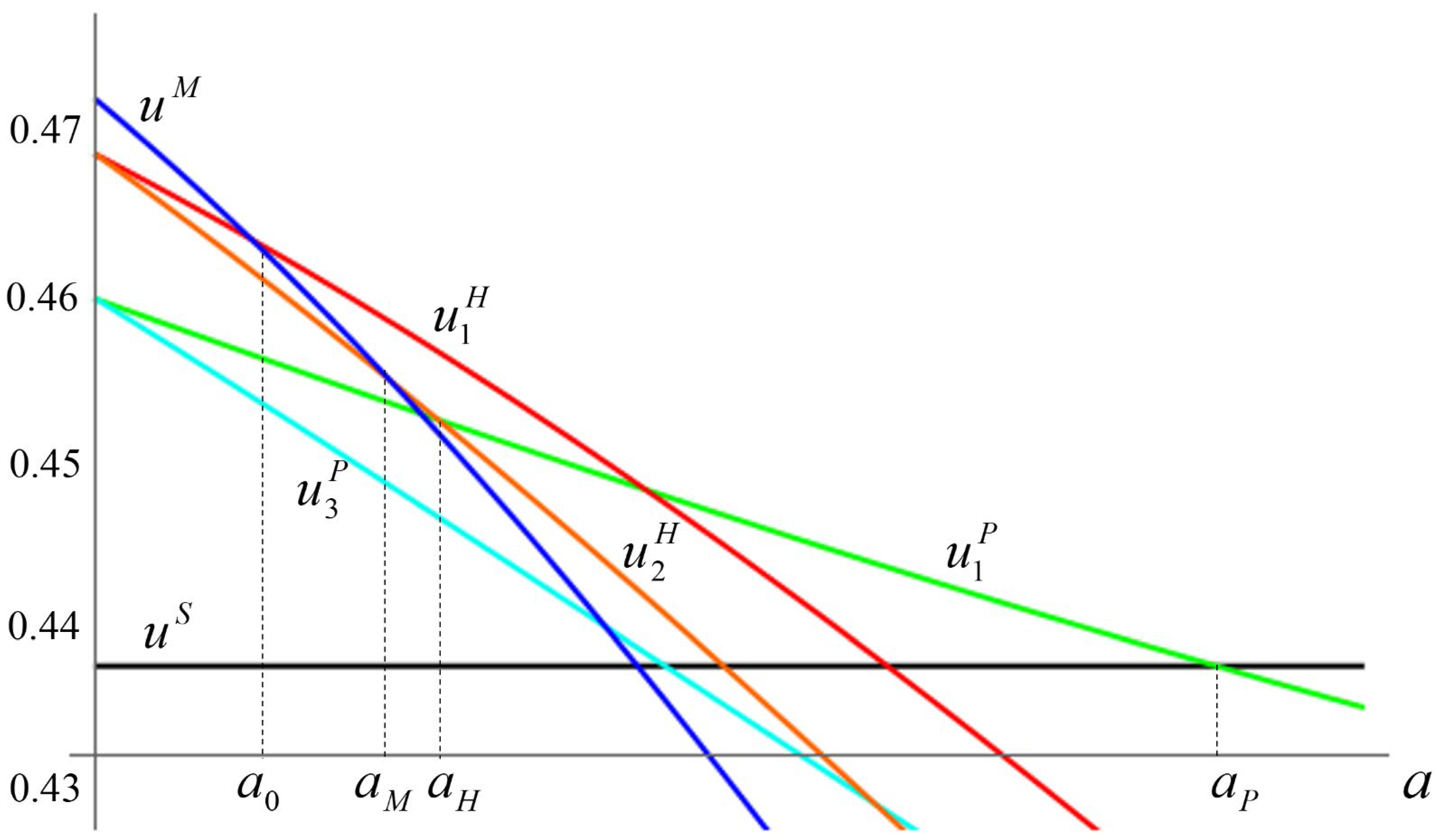
The direct R&D spillovers in the multilateral structure should provide each nation with an equilibrium payoff that is greater than the lowest equilibrium payoff that any hub-and-spoke structure produces—namely, the common payoff earned by the spokes—for a sufficiently small attrition rate. This is the relevant condition because two nations can effectively deny another nation a high payoff in a particular equilibrium by selecting another equilibrium in which both are better off. By a similar argument, the hub-and-spoke structure becomes superior to the multilateral structure for the spokes if the attrition is sufficiently high. The equilibrium for the hub-and-spoke structure then becomes coalition-proof if the common equilibrium payoffs that the spokes earn are higher than the payoffs that these nations obtain in the equilibrium for the setting with one isolated bilateral club. This should be possible since the hub-and-spoke agreement provides direct (for the hub) and indirect R&D spillover benefits relative to the restricted direct bilateral R&D spillover benefits enjoyed by the members of the isolated bilateral club. This is indeed the case for an interval of attrition rates, as the proposition below demonstrates. Finally, by continuity, the isolated bilateral club is coalition-proof for another interval of attrition rates. The upper attrition rate of this interval is the level at which the equilibrium payoff for the nations in the bilateral club is just equal to the equilibrium common equilibrium payoff that each nation can earn in the arrangement in which all nations stand alone. Figure 1 illustrates the results.
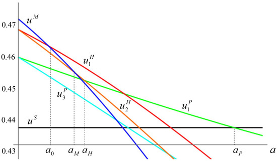
Figure 1.
Nash equilibrium payoff levels without transfers for c = 1.
Proposition 1.
For an interval of sufficiently small attrition rates, the multilateral structure is the PCPNE. For an interval of higher attrition rates, the hub-and-spoke structure is the PCPNE. For another interval of even higher attrition rates, the structure containing an isolated bilateral club is the PCPNE. Finally, for an interval of sufficiently high attrition rates, the equilibrium for the structure in which all nations stand alone is the PCPNE.
Proof.
Let and denote the Nash equilibrium payoffs in the multilateral and stand-alone structures, respectively. From Lemma 1, for , and for . From Lemma 2, for , and for . Combining the various Nash equilibria payoffs, it follows that the PCPNE is: (i) the Nash equilibrium for the multilateral structure for since for , for , for , for , for ; (ii) the Nash equilibrium for the hub-and-spoke structure for , since for and for ; (iii) the Nash equilibrium for the structure containing an isolated bilateral club for , since for and for and (iv) the Nash equilibrium for the structure containing singletons for , since for (see Figure 1 and Appendix A). □
4.2. Equilibrium with Coordinated Transfers within Clubs
We now determine the PCPNE for climate clubs in which income transfers are feasible and coordinated. Each club determines its transfers and implements them after the club members make their decisions concerning R&D efforts. We assume that each club selects the transfers to maximize the product of its members’ payoffs (i.e., the Nash-bargaining functional). The optimal transfers within any club equate the payoffs of the club members. When club members choose R&D efforts, in the second stage, they anticipate that transfers equate payoffs. Formally, we consider three-stage games of complete but imperfect information. The first and second stages are as before. In the third stage, the clubs implement transfers (see Appendix B for details).
The multilateral and hub-and-spoke structures internalize both types of externalities. The critical difference between these arrangements is the fact that the multilateral arrangement connects all nations while the hub-and-spoke arrangement connects the hub to the spokes, but the spokes do not connect. This implies that for sufficiently small attrition rates, the equilibrium for the multilateral arrangement is Pareto superior to the equilibrium for the hub-and-spoke arrangement.
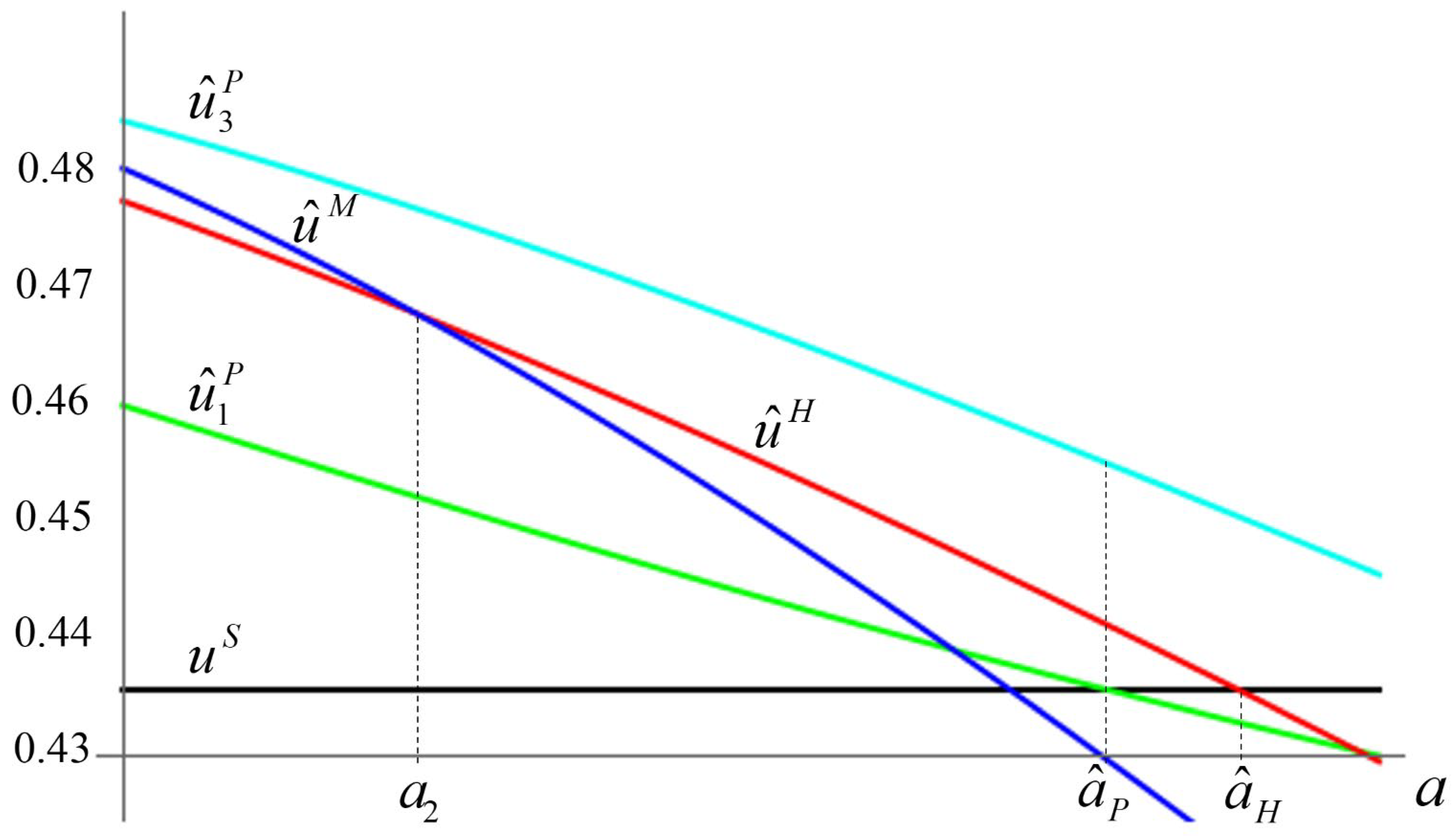
The equilibrium for the multilateral arrangement is not self-enforcing. For an interval of sufficiently low attrition rates, a single nation benefits from deviating from this arrangement, and the remaining nations also benefit from sticking together because the common equilibrium payoffs that two nations earn in the isolated bilateral club is at least as high as the payoffs these nations obtain in the stand-alone arrangement. Interestingly, when the common equilibrium payoff for the nations in the isolated bilateral club equals the stand-alone equilibrium payoff, it becomes individually rational for the free riding nation to “broker” an agreement with the other two nations in order to form the hub-and-spoke arrangement. Since all nations in the hub-and-spoke arrangement internalize externalities, the common equilibrium payoff for such an arrangement falls less quickly with the attrition rate than the common equilibrium payoff earned by the nations that belong to the isolated bilateral club. Hence, all three nations find it advantageous to select the equilibrium for the hub-and-spoke arrangement for a subsequent interval of attrition rates. Once the attrition rate erodes all benefits from R&D sharing, the PCPNE becomes the equilibrium for the stand-alone structure, see Figure 2.
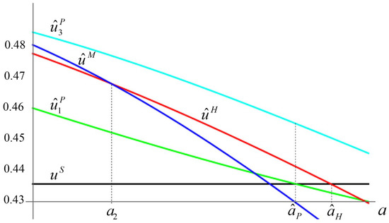
Figure 2.
Nash equilibrium payoff levels with transfers.
Proposition 2.
For sufficiently small attrition rates, the equilibrium for the setting in which there is an isolated bilateral club is the PCPNE. As attrition rates increase, the PCPNE structure is first the hub-and-spoke and later the stand-alone.
Proof.
Let , , and denote the Nash equilibrium payoffs for the multilateral, hub-and-spoke, and isolated bilateral structures, respectively. Consider the isolated bilateral structure in which nations 1 and 2 collaborate and nation 3 stands alone in what follows. Combining the PCPNE payoffs for the relevant structures, we find that the PCPNE is: (i) the Nash equilibrium for the setting in which there is an isolated bilateral club for , since for , for and at ; (ii) the Nash equilibrium for the hub-and-spoke structure for , since for and at ; (iii) the Nash equilibrium for the structure with singletons for , since (see also Figure 2 and Appendix B). □
5. Global Welfare Analysis
We now consider global welfare levels in the absence and in the presence of transfers within clubs. We let superscript index the global welfare level for each relevant club structure. The global welfare level are denoted by when agreements do not allow transfers and when agreements allow transfers.
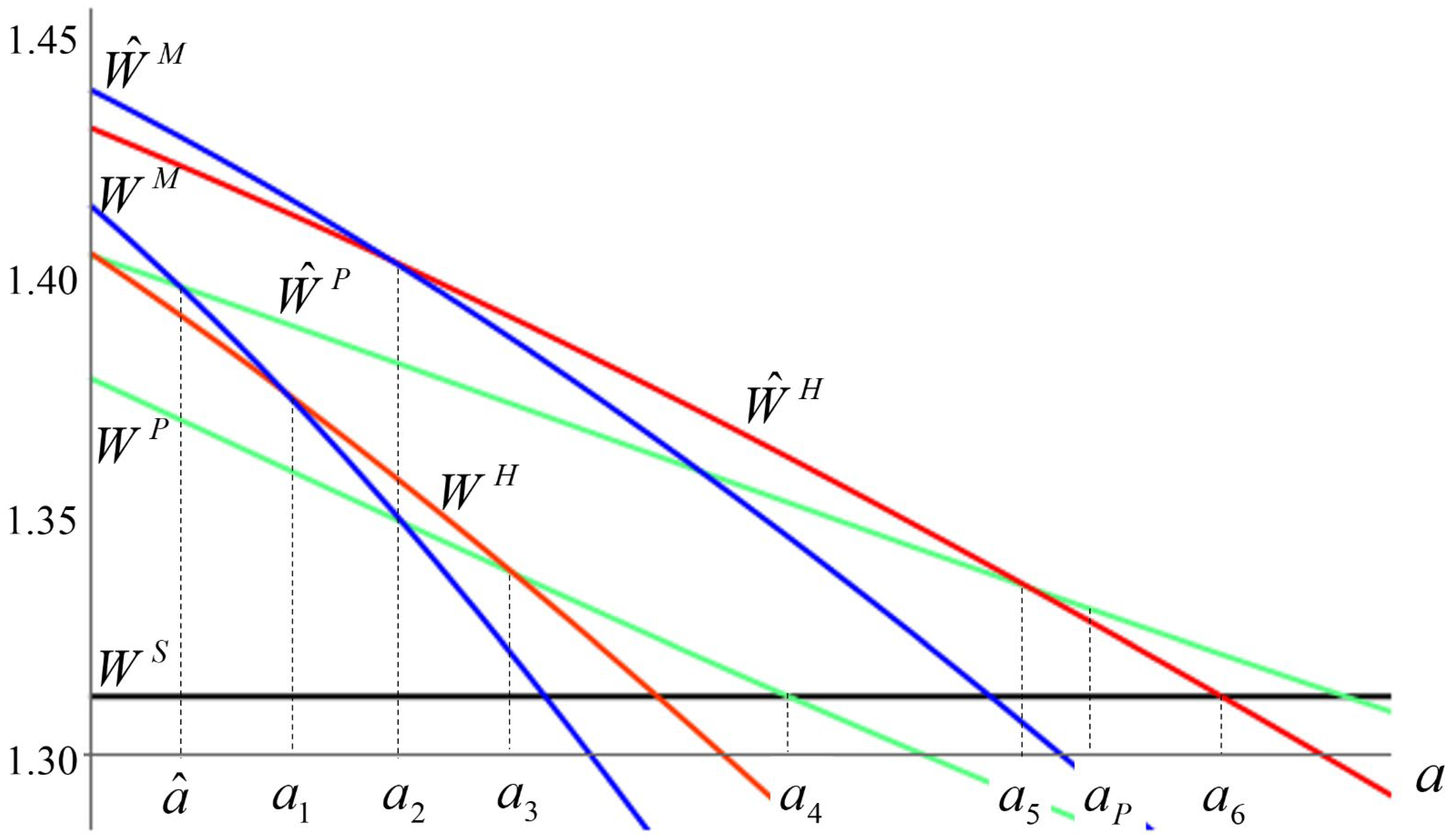
We compute the global welfare levels as functions of the attrition rate and the scale parameter. Figure 3 provides the global welfare curves and enables us to derive the following ranking of global welfare levels:
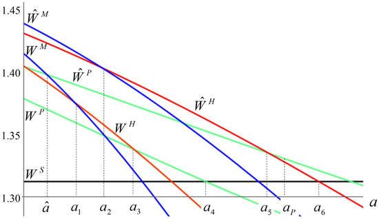
Figure 3.
Global welfare.
- (i)
- for ;
- (ii)
- for ;
- (iii)
- for ;
- (iv)
- for .
When clubs allow transfers, the ranking of global welfare levels is as follows:
- (i)
- for ;
- (ii)
- for ;
- (iii)
- for ;
- (iv)
- for ;
- (v)
- for
where the cut-off values are summarized in Table 1.

Table 1.
Cut-off attrition values.
The ranking of global welfare levels when clubs do not allow transfers capture the advantage of teamwork for sufficiently small attrition rates. As expected, the greatest benefit from teamwork is in the multilateral setting. The second-best and third-best situations are the hub-and-spoke network and the isolated bilateral club network, respectively. When clubs allow transfers, on the other hand, we observe a surprising sort of events. Unlike the well-behaved ranking order for the settings without transfers, we now see that the global welfare level in the setting with an isolated bilateral club exceeds the global welfare level in the hub-and-spoke network for an interval of attrition rates, even though for smaller attrition rates, the reverse is true. The nation outside the club in the setting with an isolated bilateral club enjoys an equilibrium payoff that is larger than the common payoff earned by all nations in the hub-and-spoke network. In addition, for an interval of attrition rates, the difference between the equilibrium payoff for the stand-alone nation and the equilibrium payoff earned by the average nation in the hub-and-spoke network exceeds the difference between the sum of equilibrium payoffs for the remaining hub-and-spoke nations and the sum of equilibrium payoffs for the bilateral club members in the isolated bilateral club structure.
One can understand the welfare analysis above in terms of what a global planner can achieve if he/she has the power to command the nations to collaborate or not in green R&D production. When collaboration improves welfare, the planner can choose which collaboration network (i.e., multilateral, hub-and-spoke, or isolated bilateral depicted) should be formed in order to take advantage of knowledge spillovers. In a more realistic scenario, however, the nations are free to make their own coordination decisions. The club structures that materialize are those that Propositions 1 and 2 predict. Hence, a non-interventionist global planner would have to be content with the global welfare levels that result from the PCPNE set.
Close inspection of Figure 3 reveals an interesting, welfare-improving avenue for policy intervention by a global planner that does not violate the nations’ ability to make their own coordination choices. Proposition 2 informs us that the Nash equilibrium for the setting with multilateral agreements is not coalition proof. Proposition 1, on the other hand, tells us that for sufficiently small attrition rates, the Nash equilibrium for the setting with multilateral agreements is coalition-proof. Hence, if a global planner is capable of deciding whether agreements should allow transfers, there is a window of opportunity to exercise his/her power for sufficiently small attrition rates. By prohibiting transfers for an interval of sufficiently small attrition rates, the planner induces the nations to select the Nash equilibrium for the setting with multilateral agreements without transfers. The global welfare improvement resulting from this smart prohibition choice is clear in Figure 3. It is equal to the horizontal distance between and for sufficiently small attrition levels (i.e., those at which the height of is at least as large as the height of ). This occurs for , where is larger for a smaller . Figure 3 also makes it clear that the global planner should allow transfers within clubs for large values of the attrition rate.
Corollary 1.
For sufficiently small attrition rates, constrained global welfare levels improve when clubs prohibit transfers because multilateral structure without transfers is self-enforcing. For larger attrition rates, constrained global welfare levels are maximal when clubs allow transfers.
6. Larger Economies
In this section, we extend our analysis to settings in which , where there are nations. We consider both clubs in which transfers are prohibited and in which transfers are allowed.
6.1. Larger Economies without Transfers
If clubs do not allow income transfers, the number and types of PCPNE increase because there are several Nash equilibria with asymmetric outcomes. The analysis is more complex, but we are able to provide some coherent results for the PCNPE and for the “second-best” structures for sufficiently low attrition rates. The purpose of this exercise is to illustrate that the stable club structures can indeed be very large, possibly encompassing all nations on the globe. There are multiple types of stable club structures depending on the value of the attrition parameter; these are summarized in Table 2.
Table 2.
Attrition ranges for the top 3 PCPNEs.
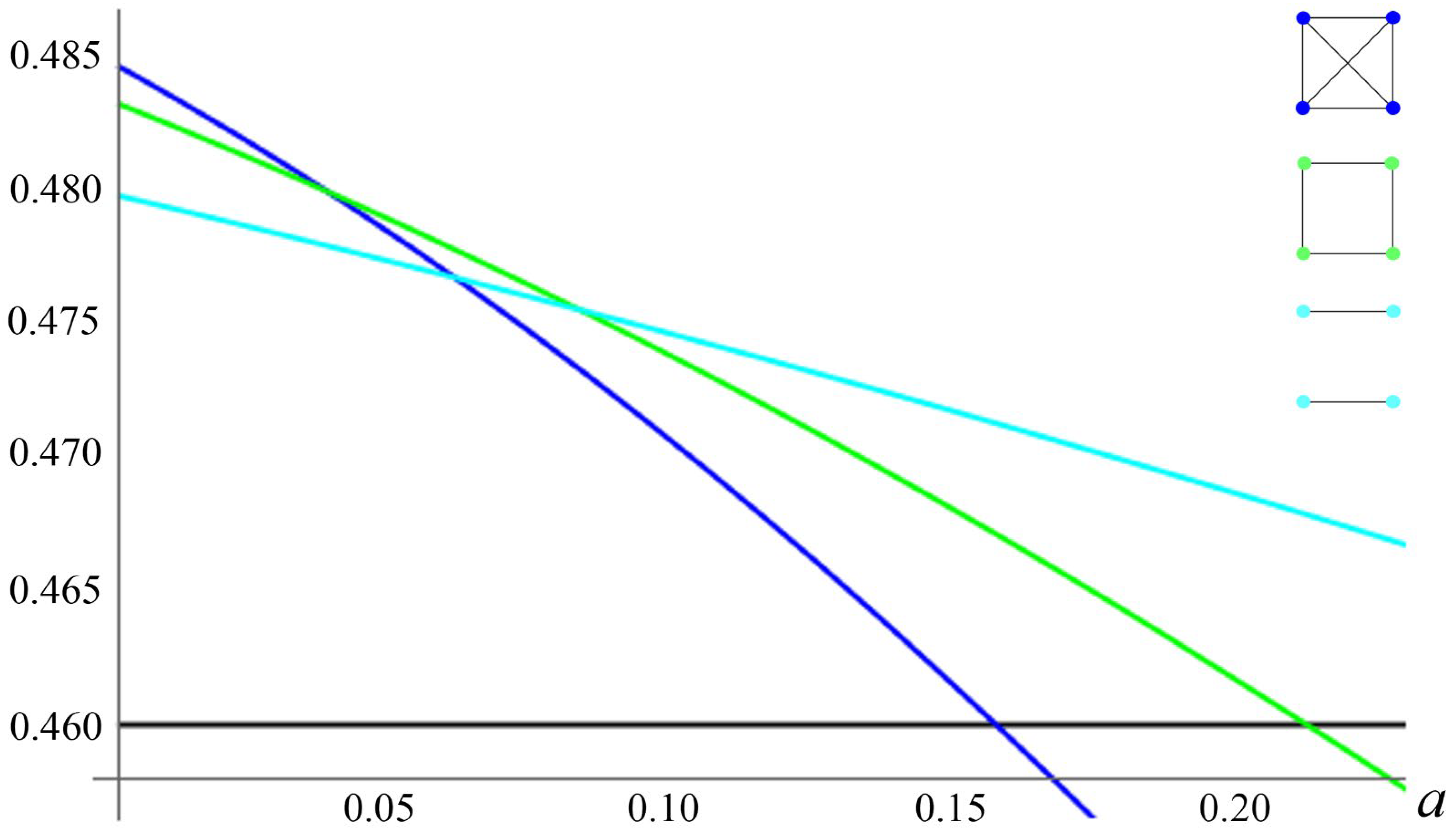
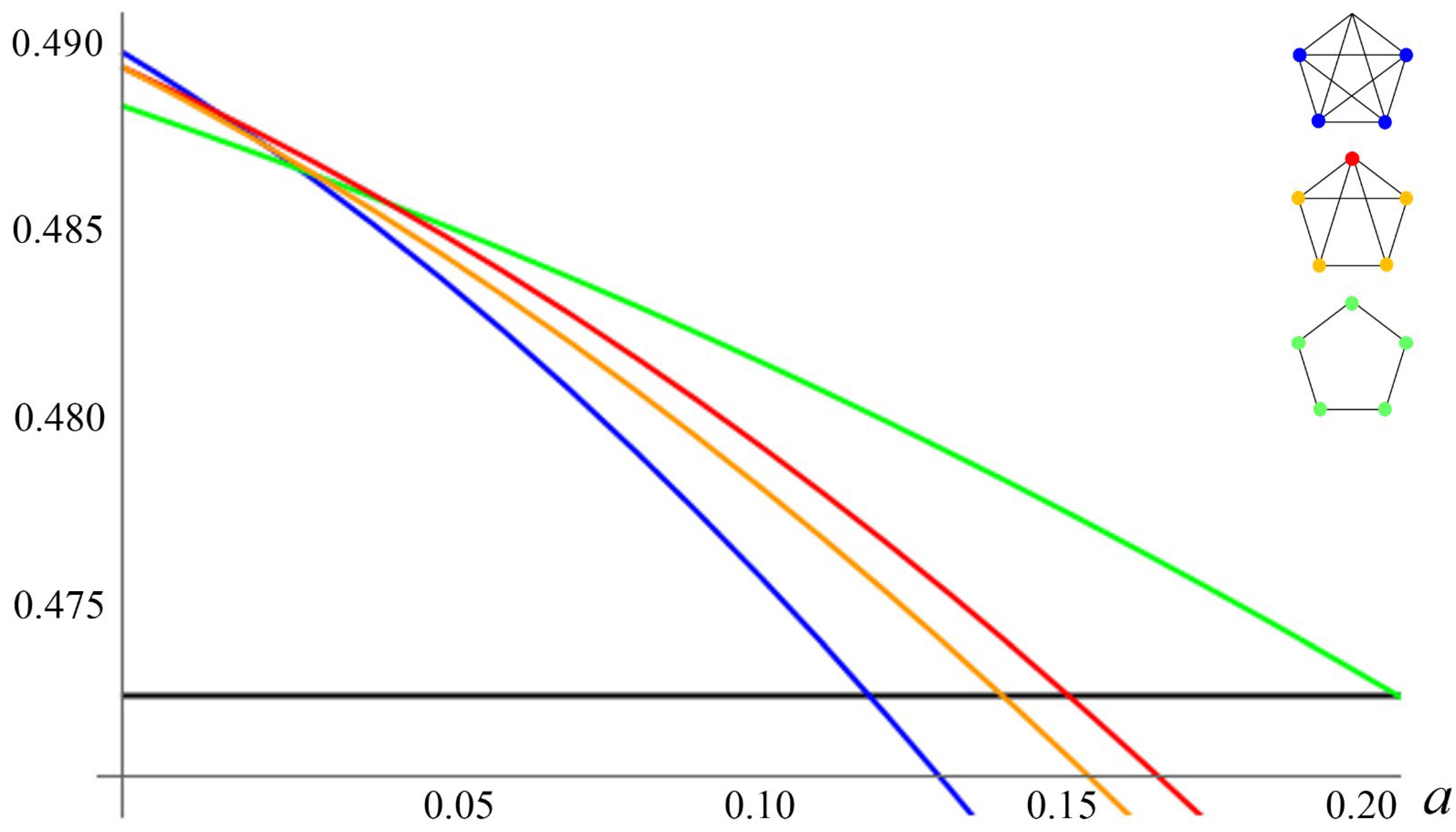
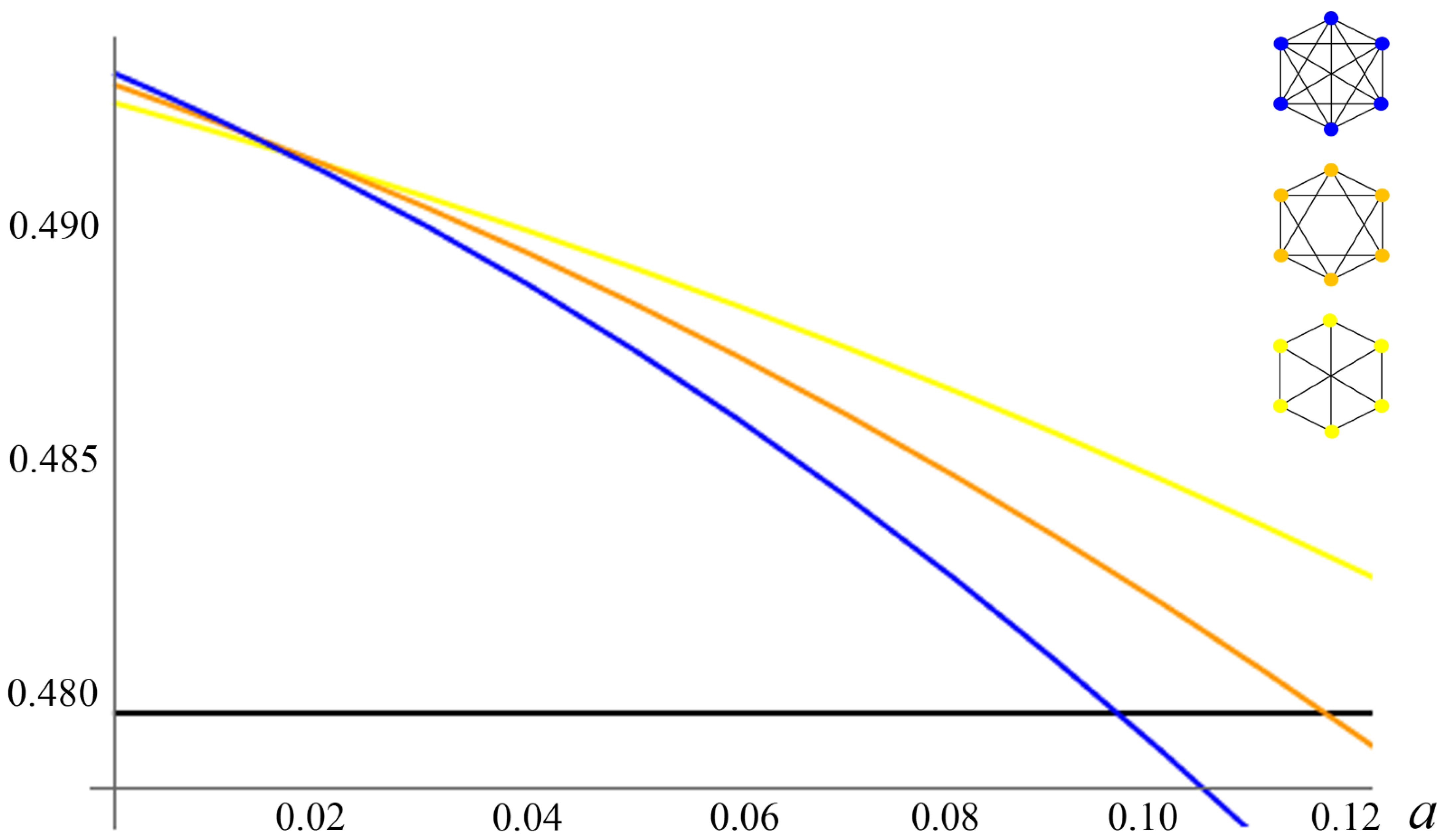
Figure 4, Figure 5 and Figure 6 illustrate the Nash equilibrium payoffs as functions of the attrition rate. Figure 4 clearly shows that the second-best stable formation is the “circle of four”, in which all nations have two links, one link to each of its two neighbors. If , Figure 5 shows that the second-best stable formation is characterized by one nation being a hub (linked to the other four nations) and the other four nations having two links. If , Figure 6 shows that in the second-best-stable formation, each nation is linked to four other nations.

Figure 4.
PCPNE for Z = 4.
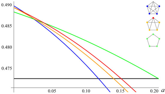
Figure 5.
PCPNE for Z = 5.

Figure 6.
PCPNE for Z = 6.
First, it is important to note that the multilateral club containing all nations is a PCPNE for sufficiently low attrition rates for economies with four, five, and six nations. If the total number of nations is odd, the second-best stable formation features a hub with a larger number of links than the spokes. If the total number of nations is even, the second-best stable formation features a symmetric composition where all nations have the same number of links.
Table 3 expands the number of nations up to 197. The cut-off attrition rates in Table 3 are those that “separate” the stable Grand Coalition and the second-best coalitional structure. By considering larger economies, with up to 197 nations, we see that the two main findings described above are consistent throughout. If the attrition is sufficiently small, the PCPNE will always involve all nations in the globe:
Table 3.
Cut-off attrition values.
Proposition 3.
For a finite number, the PCPNE will be the Grand Coalition structure as long asis sufficiently small, regardless of.
Proof.
Let , , and denote the Nash equilibrium payoffs for the multilateral structure, the second-highest payoff formation for an odd number and an even number , respectively, where the subscripts index the number of links the nation has. A straightforward calculation by using Equations (A1) and (A2) in Appendix A shows that when approaches to zero, is always greater than or , as follows:
□
This is good news for international environmental agreements in which the benefits from R&D spillovers are perfectly excludable. In addition, the second-best PCPNE alternates depending on whether or not the total number of nations is odd.
6.2. Large Economies with Transfers
Let be the number of nations that belong to clubs, with , denoting the number of stand-alone nations. We allow the formation of multiple clubs. To fixate ideas and derive some intuition, we first consider the particular case in which the attrition rate is zero. We later consider the general model in which the attrition rate is nonzero.
We summarize our findings with respect to the effect of an expansion in the number of nations on the size of a stable multilateral club in the absence of attrition in the following proposition:
Proposition 4.
In the absence of attrition (i.e., ), the larger the global economy is, the larger will be the size of the stable club , regardless of.
Proof.
Let denotes the equilibrium payoff when the nation belongs to the bilateral or multilateral club with stand-alone nations. When , the club is the PCPNE if
Let be a number such that the above condition holds as an equation and denote the maximum number of members. Then, applying the implicit function theorem at yields
□
Table 4 shows the results of our analysis under the assumption that there is no attrition and the scale parameter of the cost function is one. For economies of sizes 3 to 5, the PCPNE feature bilateral clubs and 1 to 3 stand-alone nations. For economies of sizes 6 to 8, the PCPNE are trilateral clubs with 3 to 5 stand-alone nations. Finally, for economies of sizes 196 to 198, the PCPNE feature multilateral clubs containing 70 nations and 126 to 128 stand-alone nations.
Table 4.
Stable size for a = 0 and c = 1.
One important result of the analysis is that the nations form, at most, one club. We also find that the size of the stable multilateral club increases at a decreasing rate as the size of the global economy increases. These implications follow from the fact that technological spillovers associated with collaborative R&D efforts flow to nations that join clubs only. In other words, the club good benefits club members only. Outsiders, on the other hand, enjoy the by-product, which results from knowledge creation in clubs. This by-product is the collective carbon emission reductions promoted by the club members. Therefore, there is a tension between the incentive of being a member of a club and the incentive to free ride on the emission reductions promoted by the collective efforts of club members.
The analysis demonstrates that the tension between the incentive to join the club and the incentive to free ride produces the unconventional finding that the size of a stable multilateral club increases with the size of the economy. Diamantoudi and Sartzetakis [20], whose model builds on the model advanced by Barrett [18], demonstrated that the stable coalition involves no more than four countries. More recently, Diamantoudi and Sartzetakis [21] demonstrated that if the nations have perfect foresight about group deviations, the stable coalitions can be larger and efficient. Our results are similar in this regard. We must also emphasize that our stable coalitions emerge from a refinement of Nash equilibrium. This method is quite distinct from the most common notions of coalition stability used in the literature, such as the notion of “internal and external stability” originated by d’Aspremont et al. [50]. Different methods typically generate different outcomes.
We now provide results for the general model in which and . Table 5 shows that the types of stable club structures depend crucially on the number of nations and the attrition rate . As demonstrated above, if , the resulting stable club structures will consist of a mix of multilateral and stand-alone nations, except for isolated bilateral clubs; that is, for , ,, and . The equilibrium payoff for a stand-alone nation in the singleton coalition structure increases with : it becomes larger than the common equilibrium payoff earned by bilateral nations in isolated bilateral clubs for all .
Table 5.
Stable coalition structures and ranges for the attrition rate.
For and , we see that as the attrition rate increases, the stable club structures contain, initially, a mix of bilateral or multilateral and stand-alone nations. Then, for higher attrition rates, it becomes a mix of hub-and-spoke clubs and stand-alone nations. For still higher attrition rates, it features a mix of isolated bilateral clubs and stand-alone nations. Finally, for sufficiently high attrition rates, it consists of stand-alone nations only.
7. Conclusions
Several nations are currently engaged in the production of CCS research in collaborative R&D networks. These networks are bilateral, multilateral, and hub-and-spoke. Such networks are promising additions to the Paris Agreement. Hub-and-spoke networks, in particular, may allow the hub nation to partake in knowledge spillovers from several partners. The hub nation is likely to benefit from novel and non-redundant pieces of knowledge.
Our theoretical model also builds on recent empirical findings of studies of collaborative R&D that demonstrate that the productivity of R&D collaborations may crucially depend on some aspects related to social interactions among researchers. There is evidence that productivity in research teams correlates positively to team cohesiveness. A team is more cohesive the stronger the ties are among its team members. There is also evidence that cohesive R&D collaborations develop in order to alleviate or resolve moral hazard problems within research teams. Thus, there appears to be a chain linking team efforts to alleviate inherent moral hazard problems to the level of trust shared by team members and the latter to the team’s research productivity. We incorporate these notions in our model in a synthetic form. We assume that research collaborations are typically subject to relational attrition, which erodes their efficiency rate. We also allow team size to erode the team’s efficiency rate.
We demonstrate that, conditional on the magnitude of the attrition rate, multilateral, hub-and-spoke, and isolated bilateral agreements can be stable if clubs do not allow income transfers. For sufficiently small attrition rates, multilateral clubs are Pareto-superior to other forms of agreements because the benefits generated by R&D sharing increase with the number of nations that collaborate (directly or indirectly). Hub-and-spoke clubs are second best.
If clubs allow transfers, multilateral clubs are never coalition-proof. Hub-and-spoke and isolated bilateral clubs are stable for different attrition rates. Comparing the stability results for clubs that prohibit transfers with clubs that allow transfers, we demonstrate that global welfare improves if clubs prohibit transfers for sufficiently low attrition rates.
We also considered the effects associated with enlarging the global economy. The findings depend on whether or not clubs allow transfers. If clubs allow transfers, the Grand Coalition is never stable. The size of a stable multilateral club increases as the size of the global economy expands in the absence of attrition. We also demonstrate that for positive attrition rates, all types of club structures can be stable as the size of the global economy expands. On the other hand, if clubs do not allow transfers, the Grand Coalition is stable for sufficiently small attrition rates even if the number of nations is very large. We also show that several other structures, with the participation of almost all nations on the globe, are stable depending on the value of the attrition rate. The type of “second-best” stable structure differs if the number of nations in the globe is even or odd. Our findings enable us to conjecture that the current international CCS networks may be self-enforcing and may still increase in size, even in the presence of significant attrition.
There are, at least, two important avenues for future work. First, we do not consider income or development asymmetries across nations. Given the high concentration of world income and the different development stages that we observe around the globe, one should take income or development asymmetries into account in a subsequent analysis that examines the formation and stability of climate clubs. Such an analysis will inevitably confront equity and efficiency tradeoffs, which immediately leads one to give serious consideration to valid arguments that rely on the Environmental Kuznets Curve, for example, and shall thus be prepared to incorporate political economy issues into the theoretical framework. Second, among promising future technologies to be deployed to mitigate the ill effects of global warming are geoengineering methods, such as solar radiation management, which can be utilized in conjunction or in lieu of current abatement technologies if the latter are not successful in meeting the ambitious PA goals. Incorporating geoengineering methods in the arsenal of weapons that climate clubs may utilize to mitigate global warming shall lead to interesting tradeoffs, including intertemporal choices between net-zero emission and fossil fuel utilization strategies. Future climate clubs may be fairer and broader in terms of technological options.
Author Contributions
Conceptualization, Formal analysis, Visualization, Writing, E.C.D.S. and C.Y. All authors have read and agreed to the published version of the manuscript.
Funding
This research was partially supported by JSPS KAKENHI grant numbers 16K03828 and 20K01727.
Data Availability Statement
Not applicable.
Conflicts of Interest
The authors declare no conflict of interest.
Appendix A. Proof of Proposition 1
Solving the system of first-order conditions for the singleton (i.e., structure with stand-alone nation ) yields the Nash equilibrium payoffs: . In multilateral networks containing nations, each nation forms bilateral coalitions. The first-order conditions are as follows:
which yields since for . Since the maximum number of links for members is , subtracting 1 link between nations 1 and 2 from the multilateral coalitions structure (i.e., bilateral agreements) can be characterized by Equation (A1) for and the following first-order conditions:
Setting , , and in Equations (A1) and (A2) and comparing the resulting utilities yield the corresponding cut-off attrition value for the PCPNE coalition structures.
For , we know that for and from Lemma 1 and 2, respectively. From the conditions that determine the Nash equilibria for the abovementioned contribution games, we obtain
where , , and the superscripts denote equilibrium values for respective coalitional structure, that is, Singleton, Partial (isolated bilateral), Hub & Spokes, and Multilateral. Then, we obtain the respective utilities:
Comparing these equilibrium utility levels yields that: if , if , if , and if , where cut-off values depend on a scale parameter as in Table A1.
Table A1.
Cut-off attrition values.
Table A1.
Cut-off attrition values.
| 0.5 | 0.0612 | 0.1441 | 0.1350 | 0.5667 |
| 1.0 | 0.0612 | 0.1160 | 0.1350 | 0.4426 |
| 1.5 | 0.0612 | 0.1042 | 0.1350 | 0.3969 |
| 2.0 | 0.0612 | 0.0978 | 0.1350 | 0.3726 |
Although an increase in changes the respective attrition range, starting from , the PCPNE structure is always the equilibrium for the multilateral, the hub-and-spoke, the stand-alone, and the singleton as attrition rates increase, which are summarized in Figure 1.
By subtracting another link from the multilateral structure, comparing all the corresponding utilities, and repeating a similar way, we obtain the PCPNE for nations. The results are summarized in Table 3 and Figure 4, Figure 5 and Figure 6.
Furthermore, if is an even number, the second-best stable formation is characterized by the Equation (A2) for , which implies that each nation forms bilateral coalitions, and hence, the total number of links is in the second-best coalitional structure. For an odd number: , it is impossible that each nation links up with an identical number of nations. In this case, the second-best stable formation becomes the hub-and-spoke structure, i.e., one country is a hub, linking with nations, and each spoke nation forms bilateral agreements. The corresponding equilibria can be characterized by the Equation (A1) for the hub nation and Equation (A2) for the other members. In this case, the total number of links is . These second-best stable formations and those cut-off attrition values are summarized in Table 3.
Appendix B. Proof of Proposition 2
An international arbitrator promotes the intra-coalition income transfers according to the Nash bargaining formula after observing coalition members’ non-cooperative and simultaneous contributions to the public good. In the hub-and-spoke partial coalitional structure, hub nation 1 forms bilateral coalitions, while nation(s) form singleton coalition(s). In the third stage, the arbitrator implements intra-coalitional transfers for all , coalitions. The first-order conditions to the optimization problems imply that all transfers satisfy and for , which yields
The first-order conditions for hub 1 and spoke in the second stage are
For the second-order conditions, see Appendix C.
Summing Equations (A3) and (A4) in the symmetric equilibrium with , and for , yields the Samuelson condition for nations’ hub-and-spoke structure; i.e., the sum of nations’ MRS of the public good in the LHS should equal to its MRT in the RHS:
In the multilateral partial coalitions, the solution to the arbitrator’s problem in the third stage satisfies that and , which yields the intra-coalition income transfers for as follows:
The first-order condition for in the second stage is
which yields since for , where the equilibrium variables in the existence of intra-coalitional income transfers are denoted with a hat (see also Appendix C). Summing Equation (A5) yields the Samuelson condition for members’ multilateral coalitions structure as follows:
Setting , , and in Equations (A3)–(A5) yields the resulting utilities. By subtracting another link from the abovementioned structure, comparing all the corresponding utilities and repeating a similar way, we obtain the corresponding cut-off attrition values for the PCPNE structures.
In the case of and , we obtain the following results:
where and . Then, we have the corresponding utilities as follows:
By comparing these payoffs, we obtain that: if , for , if , for , if , where cut-off values are summarized as in Table A2.
Table A2.
Cut-off attrition values.
Table A2.
Cut-off attrition values.
| 0.5 | 0.1454 | 0.4034 | 0.4832 |
| 1.0 | 0.1404 | 0.4705 | 0.5329 |
| 1.5 | 0.1365 | 0.5084 | 0.5649 |
| 2.0 | 0.1333 | 0.5323 | 0.5871 |
These results are in the proof and summarized in Figure 2.
Appendix C. Second-Order Conditions for the Maximization Problems
If there is no income transfer, then all the second-order conditions are characterized by
If there exist income transfers, the first- and second-order conditions in the hub-and-spoke club for the arbitrator’s problems, respectively, are
where , , and . From (A3) and (A4), the second-order conditions for hub 1 and spoke , respectively, are as follows:
For the multilateral coalition structures, the first- and second-order conditions for the arbitrator’s problems in the third stage, respectively, are
where and . From (A5), the second-order conditions in the second stage are as follows:
References
- Nordhaus, W. Climate Clubs: Overcoming Free-riding in International Climate Policy. Am. Econ. Rev. 2015, 105, 1339–1370. [Google Scholar] [CrossRef] [Green Version]
- Silva, E.C.D.; Kahn, C.M. Exclusion and Moral Hazard: The Case of Identical Demand. J. Public Econ. 1993, 52, 217–235. [Google Scholar] [CrossRef]
- de Coninck, H.; Stephens, J.C.; Metz, B. Global learning on carbon capture and storage: A call for strong international cooperation on CCS demonstration. Energy Policy 2009, 37, 2161–2165. [Google Scholar] [CrossRef] [Green Version]
- Herzog, H.J. Scaling up carbon dioxide capture and storage: From megatons to gigatons. Energy Econ. 2011, 33, 597–604. [Google Scholar] [CrossRef]
- Leach, A.; Mason, C.F.; Veld, K.V. T Co-optimization of enhanced oil recovery and carbon sequestration. Resour. Energy Econ. 2011, 33, 893–912. [Google Scholar] [CrossRef] [Green Version]
- The Royal Society. Knowledge, Networks and Nations: Global Scientific Collaboration in the 21st Century. 2011. Available online: https://www.comminit.com/global/content/knowledge-networks-and-nations-global-scientific-collaboration-21st-century (accessed on 15 June 2020).
- Bakker, S.J.A.; Hagemann, M.; Moltmann, S.; Palenberg, A.; de Visser, E.; Höhne, N.; Jung, M. Role of CCS in the international climate regime. Policy Stud. 2013, 2012, 2011. [Google Scholar]
- DeFazio, D.; Lockett, A.; Wright, M. The Impact of Collaboration and Funding on Productivity in Research Networks. Res. Policy 2009, 38, 293–305. [Google Scholar] [CrossRef]
- Sorenson, O.; Rivkin, J.W.; Fleming, L. Complexity, networks and knowledge flow. Res. Policy 2006, 35, 994–1017. [Google Scholar] [CrossRef]
- Forti, E.; Franzoni, C.; Sobrero, M. Bridges or isolates? Investigating the social networks of academic inventors. Res. Policy 2013, 42, 1378–1388. [Google Scholar] [CrossRef] [Green Version]
- Grannovetter, M. The Strength of Weak Ties. Am. J. Sociol. 1973, 78, 1360–1380. [Google Scholar] [CrossRef] [Green Version]
- Goyal, S. Connections: An Introduction to the Economics of Networks; Princeton University Press: Princeton, NJ, USA, 2007. [Google Scholar]
- Fershtman, C.; Gandal, N. Direct and Indirect Knowledge Spillovers: The “Social Network” of Open-Source Projects. RAND J. Econ. 2011, 42, 70–91. [Google Scholar] [CrossRef] [Green Version]
- Jackson, M.O.; Wollinsky, J. A Strategic Model of Social and Economic Networks. J. Econ. Theory 1996, 71, 44–74. [Google Scholar] [CrossRef]
- Friedlander, F. Performance and interactional dimensions of organizational work groups. J. Appl. Psychol. 1966, 50, 257–265. [Google Scholar] [CrossRef]
- Bloch, F.; Jackson, M.O. The formation of networks with transfers among players. J. Econ. Theory 2007, 133, 83–110. [Google Scholar] [CrossRef] [Green Version]
- Carraro, C.; Siniscalco, D. Strategies for the international protection of the environment. J. Public Econ. 1993, 52, 309–328. [Google Scholar] [CrossRef]
- Barrett, S. Self-Enforcing International Environmental Agreements. Oxf. Econ. Pap. 1994, 46, 878–894. [Google Scholar] [CrossRef]
- Eyckmans, J.; Tulkens, H. Simulating coalitionally stable burden sharing agreements for the climate change problem. Resour. Energy Econ. 2003, 25, 299–327. [Google Scholar] [CrossRef]
- Diamantoudi, E.; Sartzetakis, E.S. Stable International Environmental Agreements: An Analytical Approach. J. Public Econ. Theory 2006, 8, 247–263. [Google Scholar] [CrossRef] [Green Version]
- Diamantoudi, E.; Sartzetakis, E. International environmental agreements: Coordinated action under foresight. Econ. Theory 2015, 59, 527–546. [Google Scholar] [CrossRef]
- Diamantoudi, E.; Sartzetakis, E.S.; Strantza, S. International Environmental Agreements-Stability with Transfers among Countries. FEEM Working Paper. 2018, p. 20. Available online: https://www.feem.it/m/publications_pages/ndl2018-020.pdf (accessed on 18 October 2021).
- Diamantoudi, E.; Sartzetakis, E.S.; Strantza, S. International Environmental Agreements—The Impact of Heterogeneity among Countries on Stability. FEEM Working Paper. 2018, p. 22. Available online: https://www.feem.it/m/publications_pages/ndl2018-022.pdf (accessed on 18 October 2021).
- Chander, P. The gamma-core and coalition formation. Int. J. Game Theory 2007, 35, 539–556. [Google Scholar] [CrossRef]
- Osmani, D.; Tol, R. Toward Farsightedly Stable International Environmental Agreements. J. Public Econ. Theory 2009, 11, 455–492. [Google Scholar] [CrossRef]
- Silva, E.C.D.; Zhu, X. Overlapping International Environmental Agreements. Strateg. Behav. Environ. 2015, 5, 255–299. [Google Scholar] [CrossRef]
- Battaglini, M.; Harstad, B. Participation and Duration of Environmental Agreements. J. Political Econ. 2016, 124, 160–204. [Google Scholar] [CrossRef] [Green Version]
- Silva, E.C.D. Self-enforcing agreements under unequal nationally determined contributions. Int. Tax Public Financ. 2017, 24, 705–729. [Google Scholar] [CrossRef] [Green Version]
- Bayramoglu, B.; Finus, M.; Jacques, J.-F. Climate agreements in a mitigation-adaptation game. J. Public Econ. 2018, 165, 101–113. [Google Scholar] [CrossRef] [Green Version]
- Breton, M.; Sbragia, L. The Impact of Adaptation on the Stability of International Environmental Agreements. Environ. Resour. Econ. 2019, 74, 697–725. [Google Scholar] [CrossRef] [Green Version]
- Finus, M.; Furini, F.; Rohrer, A.V. The efficacy of international environmental agreements when adaptation matters: Nash-Cournot vs Stackelberg leadership. J. Environ. Econ. Manag. 2021, 109, 102461. [Google Scholar] [CrossRef]
- Greaker, M.; Hoel, M. Incentives for Environmental R&D. CREE Working Paper. 2011, p. 1. Available online: https://www.cree.uio.no/publications/CREE_working_papers/pdf_2011/envrd_22august2011_wp1_2011.pdf (accessed on 18 October 2021).
- Golombek, R.; Hoel, M. International Cooperation on Climate-friendly Technologies. Environ. Resour. Econ. 2011, 49, 473–490. [Google Scholar] [CrossRef] [Green Version]
- Finus, M.; Rundshagen, B. Endogenous coalition formation in global pollution control: A partition function approach. In The Endogenous Formation of Economic Coalitions; Edward Elgar Publishing: Northampton, MA, USA, 2003. [Google Scholar]
- Mukunoki, H.; Tachi, K. Multilateralism and Hub-and-Spoke Bilateralism. Rev. Int. Econ. 2006, 14, 658–674. [Google Scholar] [CrossRef]
- Saggi, K.; Yildiz, H. Bilateralism, multilateralism, and the quest for global free trade. J. Int. Econ. 2010, 81, 26–37. [Google Scholar] [CrossRef] [Green Version]
- Hur, J.; Alba, J.D.; Park, D. Effects of Hub-and-Spoke Free Trade Agreements on Trade: A Panel Data Analysis. World Dev. 2010, 38, 1105–1113. [Google Scholar] [CrossRef] [Green Version]
- Bernheim, B.; Peleg, B.; Whinston, M.D. Coalition-Proof Nash Equilibria I. Concepts. J. Econ. Theory 1987, 42, 1–12. [Google Scholar] [CrossRef]
- Finus, M.; Rundshagen, B. Mumbership Rules and Stability of Coalition Structures in Positive Externality Games. Soc. Choice Welf. 2009, 32, 389–406. [Google Scholar] [CrossRef]
- Nagase, Y.; Silva, E.C. Acid rain in China and Japan: A game-theoretic analysis. Reg. Sci. Urban Econ. 2007, 37, 100–120. [Google Scholar] [CrossRef]
- Silva, E.C.; Yamaguchi, C. Interregional competition, spillovers and attachment in a federation. J. Urban Econ. 2010, 67, 219–225. [Google Scholar] [CrossRef] [Green Version]
- Silva, E.C.; Zhu, X. Emissions trading of global and local pollutants, pollution havens and free riding. J. Environ. Econ. Manag. 2009, 58, 169–182. [Google Scholar] [CrossRef]
- Spence, A.M. Cost Reduction, Competition, and Industry Performance. Econometrica 1984, 52, 101–121. [Google Scholar] [CrossRef]
- Katz, M.L. An Analysis of Cooperative Research and Development. RAND J. Econ. 1986, 17, 527–543. [Google Scholar] [CrossRef]
- d’Aspremont, C.; Jacquemin, J. Cooperative and Noncooperative R and D in a Duopoly with Spillovers. Am. Econ. Rev. 1988, 78, 1133–1137. [Google Scholar]
- Yi, S.-S.; Shin, H. Endogenous formation of research coalitions with spillovers. Int. J. Ind. Organ. 2000, 18, 229–256. [Google Scholar] [CrossRef] [Green Version]
- Huang, C.-C. Knowledge sharing and group cohesiveness on performance: An empirical study of technology R&D teams in Taiwan. Technovation 2009, 29, 786–797. [Google Scholar] [CrossRef]
- Dailey, R.C. The Role of Team and Task Characteristics in R&D Team Collaborative Problem Solving and Productivity. Manag. Sci. 1978, 24, 1579–1588. [Google Scholar]
- Bruns, H.C. Working Alone Together: Coordination in Collaboration across Domains of Expertise. Acad. Manag. J. 2013, 56, 62–83. [Google Scholar] [CrossRef]
- d’Aspremont, C.; Jacquemin, J.; Gabszeweiz, J.; Weymark, J.A. On the stability of collusive price leadership. Can. J. Econ. 1983, 16, 17–25. [Google Scholar] [CrossRef] [Green Version]
Publisher’s Note: MDPI stays neutral with regard to jurisdictional claims in published maps and institutional affiliations. |
© 2021 by the authors. Licensee MDPI, Basel, Switzerland. This article is an open access article distributed under the terms and conditions of the Creative Commons Attribution (CC BY) license (https://creativecommons.org/licenses/by/4.0/).