Testing Game Theory of Mind Models for Artificial Intelligence

Abstract

In this article, we investigate the relative performance of artificial neural networks and structural models of decision theory by training 69 artificial intelligence models on a dataset of 7080 human decisions in extensive form games. The objective is to compare the predictive power of AIs that use a representation of another agent’s decision-making process in order to improve their own performance during a strategic interaction. We use human game theory data for training and testing. Our findings hold implications for understanding how AIs can use constrained structural representations of other decision makers, a crucial aspect of our ‘Theory of Mind’. We show that key psychological features, such as the Weber–Fechner law for economics, are evident in our tests, that simple linear models are highly robust, and that being able to switch between different representations of another agent is a very effective strategy. Testing different models of AI-ToM paves the way for the development of learnable abstractions for reasoning about the mental states of ‘self’ and ‘other’, thereby providing further insights for fields such as social robotics, virtual assistants, and autonomous vehicles, and fostering more natural interactions between people and machines.

1. Introduction

Developing an effective theory of collective intelligence is a considerable challenge for both artificial intelligence (AI) and social psychology; see, for example, Wolpert et al. [1], Suran et al. [2], or Kameda et al. [3]. One aspect of this challenge comes from the tension between the individual competency of an agent and the co-ordination of group behaviour that allows for the collective output to be of higher quality than any individual agent. Some important contributing factors are already understood from social psychology, for example, the topology of a social network is important, as shown by Momennejad [4], as is the fractal-like scaling of social group sizes, as shown by Harré and Prokopenko [5]. Work by Woolley et al. [6] demonstrated this tension between the individual and the collective: individual skill and effort contribute most to a group’s outcome, but performance is also improved by individual members possessing a capacity for Theory of Mind (ToM), the ability to infer the internal cognitive states of other agents, as shown in the work of Frith [7]. This leads to questions regarding the incentive structure, such as which rewards optimise group performance, a question that was studied by Mann and Helbing [8] using game theoretical mechanisms.

The relationship between game theory and ToM has been developed extensively beginning with Yoshida et al. [9] establishing foundational results. More recent work by researchers in the Meta Team et al. [10] developed the AI Cicero that uses a representation of other agents’ strategies in order to play the game of Diplomacy at a strong human level. The type of opponent decision making used in their KL-divergence module piKL is closely related to the entropic methods of games against nature described by Grünwald et al. [11] and the MaxEnt methods of game theory developed in Wolpert et al. [12]; see, for example, the recent review of inverse reinforcement learning algorithms for an AI-ToM in Ruiz-Serra and Harré [13]. This ‘game theory of mind’ perspective has proliferated in recent years. In Lee [14] and Lee and Seo [15], game theory is used in behavioural studies of macaque monkeys to test for a ToM in animals; in AI research, Bard et al. [16] suggest that ToM is a necessary element for success in complex games such as Hanabi; in social psychology, Ho et al. [17] posit that ToM is a part of planning via the need to change others’ thoughts and actions; and some of the psychological aspects are reported in Harré [18].

With that in mind, we also note that there are multiple scales at which an AI can be formulated with ‘neural’ reality being balanced against ‘psychological’ reality [19,20,21], in particular, the ‘dynamical minimalism’ suggested by Nowak [22]. That psychological phenomena are an emergent property of biological neural networks embedded in an environment is not controversial, but it has only been relatively recently that studies have shown how this may come about. For example, ADHD-related changes in brain function have been shown to have an impact on global, low-dimensional manifold dynamics [23]. These attractor dynamics have also been used to explain memory [24] and decision making [25,26,27] in biological neural networks, as well as extracting psychological phenomena from artificial neural networks [28].

In this spirit, the control parameters of the AI models used in the current study are akin to the ‘…slow dynamical variables that dominate the fast microscopic dynamics of individual neurons and synapses’ [29]. As such, it is not always necessary to model microscopic elements explicitly in an AI in order to test psychological models in and of themselves. Thus, here we model decision making at a high level, where learning is by gradient descent on macroscopic parameters. These parameters are not arbitrary though; instead, they are representations of known psychological properties and have explicit interpretations: as constraints, preferences, beliefs, desires, etc. This is because it can be informative to study the learning and decision-making process from a point of view that allows us to explicitly encode psychological factors that do not have an immediate or obvious mapping to the microscopic neurobiology of the emergent phenomenology.

With the previous discussion in mind, neural level models can make it difficult to explain the structural elements of decision making that mathematical models can make explicit. An example is the modelling of non-strategic decisions in the work of Peterson et al. [30] where they gathered data on 9831 distinct ‘problems’ in order to evaluate formal models of decision making: 12 expected utility (EU) models and a further 8 prospect theory (PT) models that extend the EU models. Peterson et al. [30] also included an unconstrained artificial neural network (ANN) that, as would be expected, performed better than any of the structural models in their analysis and could act as a performance benchmark for comparative analysis, an approach we duplicate in this work. They showed that with sufficient data, new theories can be discovered that shed light on centuries of earlier theoretical work.

In this work, we adapt the formal decision theory models of Peterson et al. [30] to the task of using an AI-ToM to model the first player’s decisions in the extensive form game data of human subjects from Ert et al. [31] (see the website of Ert: https://economics.agri.huji.ac.il/eyalert/choice (accessed on 15 October 2023). The goal is to evaluate which AI-ToM decision models most effectively predict first mover choice in extensive form games, tested against several artificial neural network models that do not have an explicit ToM aspect, but that do have complete knowledge of the players’ choices and the games’ payoffs. In contrast, AI-ToM models are highly structured decision models that explicitly include the constraints of the second player’s decision making. This evaluates constrained AI-ToM models against the theoretical best ANN models available, but the unconstrained neural network has no explanatory power, whereas the structural models have well-studied and often psychologically grounded explanations. The main limitation of this study is in the nature of the experimental games: ‘game theory of mind’ is a very specific form of ToM and a more complete test of an AI-ToM would be based in a naturalistic setting.

2. Materials and Methods

In this section, we introduce the games that the human subjects played in the original article by Ert et al. [31], describing the incentives for each decision and how the incentive structures can categorise the games. We then introduce the payoff model, Equation (1), in which the parameters of the players’ payoff function are introduced, again following [31]. The expected utility decision models and then their prospect theory modifications are introduced in the last two subsections.

2.1. Game Structure

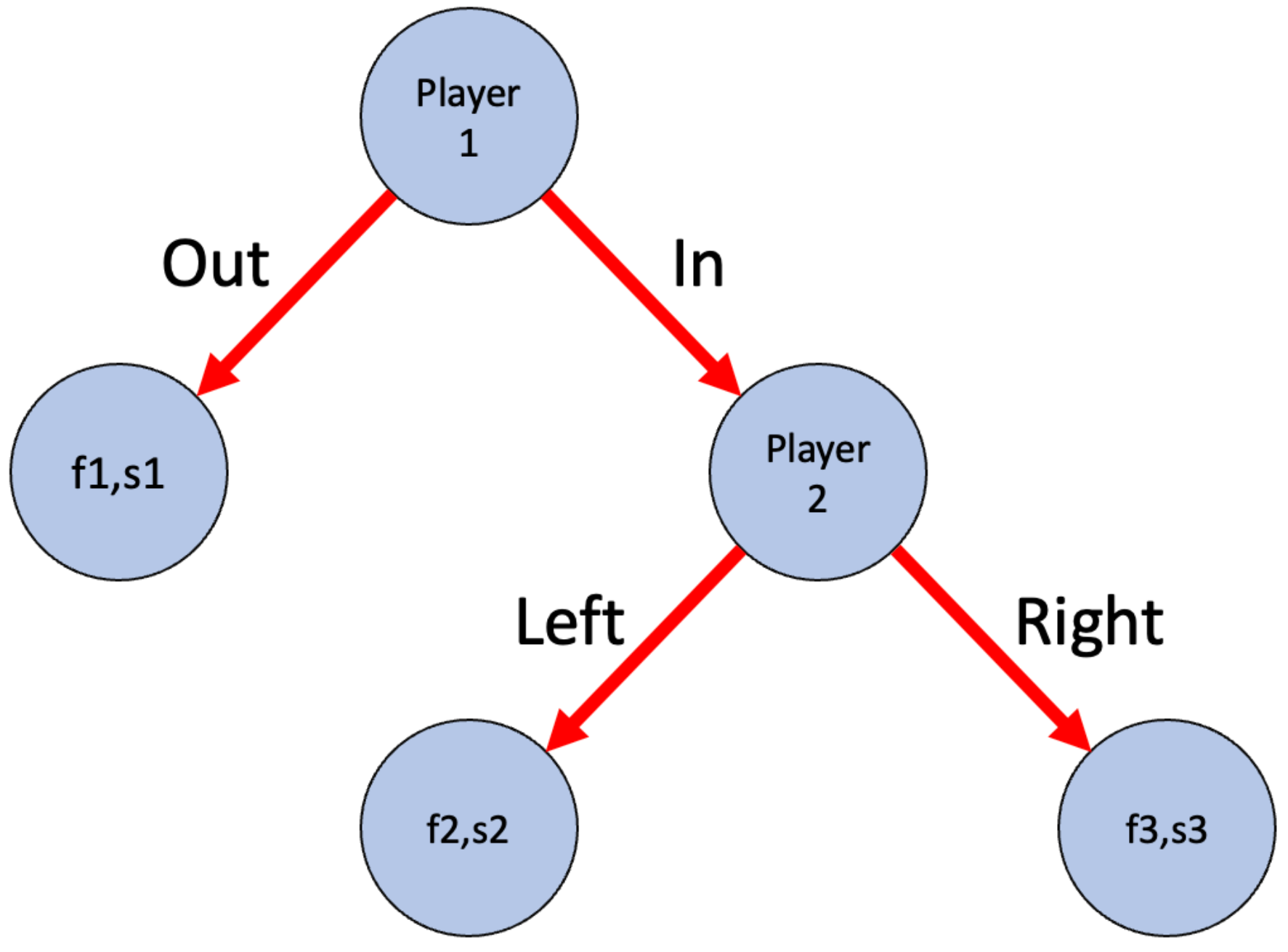
The structure of the interaction between two agents and the labelling convention is shown in Figure 1.

The games that were played can be categorised according to the relative relationships between the payoffs for the various joint strategies $\{f_i,s_j\}$ for $i,j\in \{1,2,3\}$. Game categories are not uniquely identified, and some game configurations can belong to multiple categories, see Ert et al. [31] for further details:

• All: all choices are combined without differentiating between games in which they were made.
• Common Interest: there is one option that is best for both players, e.g., $f_3>f_1>f_2$ and $s_3>s_2>s_1$.
• Safe Shot: “In” is the optimal choice for player 1, e.g., $f_2>f_3>f_1$ and $s_3>s_2>s_1$.
• Strategic Dummy: player 2 cannot affect the payoffs, e.g., $f_1>f_2=f_3$ and $s_2=s_3>s_1$.
• Near Dictator: the best payoff for player 1 is independent of player 2’s choice, e.g., $f_1>f_3>f_2$ and $s_2>s_1>s_3$.
• Free Punish: player 2 can punish player 1’s “In” choice with no cost, e.g., $f_2>f_1>f_3$ and $s_1>s_2=s_3$.
• Rational Punish: punishing player 1’s “In” choice maximises player 2’s payoff, e.g., $f_3>f_1>f_2$ and $s_1>s_2>s_3$.
• Costly Punish: punishing player 1’s “In” choice is costly, e.g., $f_3>f_1>f_2$ and $s_1>s_3>s_2$.
• Free Help: improving the other’s payoff is not costly, e.g., $f_1=f_2>f_3$ and $s_2>s_1>s_3$.
• Costly Help: improving the other’s payoff is costly for the helper, e.g., $f_3>f_1>f_2$ and $s_2>s_1=s_3$.
• Trust Game: choosing “In” improves 2’s payoff but reciprocation is irrational for player 2, e.g., $f_2>f_1>f_3$ and $s_3>s_2>s_1$ (Trust is a subset of Costly Help).
• Conflicting Interest: player 1’s reward is maximised only if player 2 chooses suboptimally after player 1 plays “In”, i.e., $f_2>f_3$ but $s_2<s_3$, while “Out” is neither minimal nor maximal for player 1, e.g., $f_3>f_1>f_2$ and $s_2>s_1>s_3$.

2.2. Experimental Data and Decision Model

The data used are from the Ert et al. [31] study where the experimental setup is as follows. A total of 116 students were recruited to play extensive form games from a selection of 240 total games, and four independent sessions were run; presented in Table 2 are the games of Ert et al. [31], and the original article also has the complete study protocols. All parametric learning is carried out using gradient descent.

We use the same function as Ert et al. [31] in which their core assumption is an inequity aversion model developed in Fehr and Schmidt [32] where individuals incur a loss of utility based on differences between their outcomes and the outcomes of others. In this sense, the specific value player 1 associates with a joint choice $\{f_i,s_j\}$ is given by:

$$x_i\equiv T(f_i,s_j)=f_i-\alpha max(s_j-f_i,0)-\beta max(f_i-s_j,0),$$

(1)

where $f_i\in \{f_1,f_2,f_3\}$ and $s_j\in \{s_1,s_2,s_3\}$ and arguments are reversed for player 2. The $\alpha$ term provides weights for disadvantageous inequality and the $\beta$ term provides weights for advantageous inequality. These parameters are discovered via gradient descent in the training phase. Note that, in the case where $\alpha =\beta =0$, this simplifies to the first argument: $T(f_i,s_j)\equiv f_i$. In Section 2.3 and Section 2.4, the utilities $U(·)$ and prospect theory models $\pi \left(p\right(·\left)\right)$ are defined, but first we define the probability of player 2 choosing “left” (L) or “right” (R), from which we can derive player 1’s probability of choosing “in” (I) or “out” (O):

$$\begin{array}{cc}\hfill U_2\left(\mathrm{L}\right)& =U\left(T(s_2,f_2)\right)\hfill \end{array}$$

(2)

$$\begin{array}{cc}\hfill U_2\left(\mathrm{R}\right)& =U\left(T(s_3,f_3)\right)\hfill \end{array}$$

(3)

$$\begin{array}{cc}\hfill p\left(\mathrm{L}\right)& =\frac{exp\left({\eta }_2{U}_2\left(\mathrm{L}\right)\right)}{exp\left({\eta }_2{U}_2\left(\mathrm{L}\right)\right)+exp\left({\eta }_2{U}_2\left(\mathrm{R}\right)\right)}\hfill \end{array}$$

(4)

$$\begin{array}{cc}\hfill U_1\left(\mathrm{O}\right)& =U\left(T(f_1,s_1)\right)\hfill \end{array}$$

(5)

$$\begin{array}{cc}\hfill U_1\left(\mathrm{I}\right)& =\pi \left(p\left(\mathrm{L}\right)\right)U\left(T(f_2,s_2)\right)+\pi \left(p\left(\mathrm{R}\right)\right)U\left(T(f_3,s_3)\right)\hfill \end{array}$$

(6)

$$\begin{array}{cc}\hfill p\left(\mathrm{I}\right)& =\frac{exp\left({\eta }_1{U}_1\left(\mathrm{I}\right)\right)}{exp\left({\eta }_1{U}_1\left(\mathrm{I}\right)\right)+exp\left({\eta }_1{U}_1\left(\mathrm{O}\right)\right)}\hfill \end{array}$$

(7)

Note that player 1’s decision model includes their (subjective) model of player 2’s (subjective) preferences and constraints [33]. The ${\eta }_i$ terms parameterise uncertainty in choices.

2.3. Expected Utility Models

EU models can incorporate arbitrary transformations $U(·)$ of outcome x, such that their utility is regarded subjectively, and $V\left(x\right)={\sum }_i{p}_{i}U\left(x_i\right)$. In general, different forms of $U(·)$ are typically non-linear, monotonic, parametric functions, and we evaluated 11 parametric forms of $U(·)$. Next are descriptions of the 5 neural networks and the 8 mathematical functions of the AI models in Peterson et al. [30] that are further modulated by different prospect theory models.

UNN: unconstrained neural network. The UNN model is a multi-layer perceptron with 5 layers: a 6 neuron input layer (one for each for the 2 players’ payoffs), 1 neuron output, and 3 hidden layers with 5, 10, and 10 neurons each. Model weights are randomly initialised in the range [0,1]. Training is conducted on a 50% subset of the data with the remainder reserved for model testing. $tanh(·)$ activation functions are used in the classifier network. The RMSE is then the observed root mean square error in the predicted choice of player 1 against observation (the RMSE is used throughout for gradient descent).

UNN Feature Engineering: an unconstrained neural network with feature engineering on the payoffs. Rather than consider the individual payoffs for each game directly (as in the unconstrained network), this model takes comparisons between a subset of the payoffs; namely ($f_1-f_2$), ($f_1-f_3$), ($f_2-f_3$), ($s_1-s_2$), ($s_1-s_3$), and ($s_2-s_3$). This network is defined as a multi-layer perceptron comprising 5 layers: a 6 node input layer (the defining payoffs of each game), a single node output layer, and 25 hidden nodes across the remaining hidden layers (5,10,10).

EU NN: an expected utility neural network without a PT model. The aim of this method is to estimate a suitable non-linear form of the utility function from game data. Following the convention of the non-neural models, a softmax function is used to select between the two outcomes based on the expected utilities of the two choices each player faces. The model’s parameters (advantageous inequity and disadvantageous inequity), and the softmax sensitivity parameter are all estimated using gradient descent along with the neural network weights. This is achieved with a 4 layer neural net including 1 neuron input, 1 neuron output, and 2 hidden layers with 5 and 10 neurons in the hidden layers. ReLU activation functions are employed in the network. The results are not significantly sensitive to these parameter choices.

MoT NN: mixture of theories neural network. This builds on the MoT model presented in Peterson et al. [30]—namely, it employs a ‘mixture of experts’ neural network architecture, where the neural network considers a subset of models, and selects between them based on the payoffs $\{f_1,f_2,f_3,s_1,s_2,s_3\}$. In this specification, the MoT model was designed to select between a generalised linear EU model, a Kahneman–Tversky PT model, an expected value model, and a Kahneman–Tversky PT model fixed at unit values. The latter two were employed because they are the simplest among the EU and PT models (i.e., no free parameters) and reduce the complexity of the model. The former two models were chosen because they are among the most stable models for the simple specifications examined. The MoT model is defined as a multi-layer perceptron comprising 5 layers: a 6 node input layer (the defining payoffs of each game), 1 node output layer, and 3 hidden layers with 5, 10, and 10 neurons each. ReLU activation functions are employed in the classifier network.

EU NN + PT NN: the EU NN with an additional neural network for learning a PT model. The EU NN uses unmodified probability weightings in the calculation of expected utilities, and the ‘Prospect Theory Neural Network’ also includes a prospect theory function around the input probabilities. Similar to the EU NN model, the prospect theory function is defined as a multi-layer perceptron comprising 4 layers: a single node input layer (the probability outcome), a single node output layer, and 2 hidden layers with 5 and 10 neurons each. ReLU activation functions are employed in the network and hyperparameter tuning is conducted through a Gaussian processes Bayesian optimiser. In this model, the network weights for both functions are optimised simultaneously using gradient descent.

The following mathematical models are highly structured and each has their own extensive history as noted by Peterson et al. [30]. The advantage of these is that their structure is motivated by specific conceptualisations regarding how decisions are made and what information is taken in and then manipulated in the decision-making process, a view that is not easily taken using conventional ANNs.

Akin to the previously described neural network models, the listed functions that follow are obtained from Peterson et al. [30]:

• Linear Model:

  $$U\left(x\right)=\lambda x$$

  (8)
• Linear Loss Aversion Behaviour:

  $$U\left(x\right)=\left\{\begin{array}{cc}x,\hfill & \mathrm{if}x\ge 0,\hfill \\ \lambda x,\hfill & \mathrm{if}x<0.\hfill \end{array}\right.$$

  (9)
• General Linear Loss Aversion Behaviour:

  $$U\left(x\right)=\left\{\begin{array}{cc}\alpha x\hfill & \mathrm{if}x\ge 0\hfill \\ \lambda \beta x\hfill & \mathrm{if}x<0\hfill \end{array}\right.$$

  (10)
• Normalised Exponential Loss Aversion Behaviour,

  $$U(x,\alpha )=\left\{\begin{array}{cc}1-e^{-\alpha x}\hfill & \mathrm{if}x\ge 0,\alpha >0\hfill \\ x,\hfill & \mathrm{if}x\ge 0,\alpha =0\hfill \\ e^{-\alpha x}-1\hfill & \mathrm{if}x\ge 0,\alpha <0\hfill \\ -\lambda (1-e^{-\alpha x})\hfill & \mathrm{if}x<0,\alpha >0\hfill \\ -\lambda x,\hfill & \mathrm{if}x<0,\alpha =0\hfill \\ -\lambda (e^{-\alpha x}-1)\hfill & \mathrm{if}x<0,\alpha <0\hfill \end{array}\right.$$

  (11)
• Power Law Loss Aversion Behaviour:

  $$U\left(x\right)=\left\{\begin{array}{cc}{x}^{\alpha }\hfill & \mathrm{if}x\ge 0\hfill \\ -\lambda {(-x)}^{-\beta }\hfill & \mathrm{if}x<0\hfill \end{array}\right.$$

  (12)
• General Power Loss Aversion Behaviour:

  $$U\left(x\right)=\left\{\begin{array}{cc}\beta x^{\alpha }\hfill & \mathrm{if}x\ge 0\hfill \\ -\lambda {(-\delta x)}^{\gamma }\hfill & \mathrm{if}x<0\hfill \end{array}\right.$$
• Exponential Power Loss Aversion Behaviour:

  $$U\left(x\right)=\left\{\begin{array}{cc}\gamma -exp(-\beta x^{\alpha })\hfill & \mathrm{if}x\ge 0\hfill \\ -\lambda (\gamma -exp(-\beta {(-x)}^{\alpha }))\hfill & \mathrm{if}x<0\hfill \end{array}\right.$$

  (13)
• Quadratic Loss Aversion Behaviour:

  $$U\left(x\right)=\left\{\begin{array}{cc}\alpha x-x^2\hfill & \mathrm{if}x\ge 0\hfill \\ -\lambda (-\beta x-x^2)\hfill & \mathrm{if}x<0\hfill \end{array}\right.$$

  (14)

2.4. Prospect Theory Models

Following Peterson et al. [30], the below PT models are employed to transform the modelled probability judgements:

• None: $\pi \left(p\right)=p$
• Kahneman–Tversky: $\pi \left(p\right)=p^{\alpha }{(p^{\alpha }+{(1-p)}^{\alpha })}^{-1/\alpha }$
• Log-Odds Linear: $\pi \left(p\right)=\beta p^{\alpha }{(\beta p^{\alpha }+{(1-p)}^{\alpha })}^{-1}$
• Power law: $\pi \left(p\right)=\beta p^{\alpha }$
• NeoAdditive: $\pi \left(p\right)=\beta +\alpha p^{\alpha }$
• Hyperbolic Log: $\pi \left(p\right)={(1-\alpha +logp)}^{\frac{\beta }{\alpha }}$
• Exponential Power: $\pi \left(p\right)=exp(-\frac{\alpha }{\beta }(1-p^{\beta })$
• Compound Invariance: $\pi \left(p\right)=exp\left(\beta {(-logp)}^{\alpha }\right)$
• Constant Relative Sensitivity: $\pi \left(p\right)={\beta }^{(1-\alpha )}+p^{\alpha }$

3. Results

3.1. Average Root Mean Square Error of Utility Models

Our first results, shown in Figure 2 and Figure 3, measure the performance of the utility models of the eight parameterised utility models compared with the five neural network models. The 13 models were each run 50 times using all of the PT models and across all game types, and the box and whisker plots report the distribution of the 13 models’ performance.

We note that in the training phase of Figure 2, the unconstrained neural network (UNN) performed the best out of all models, and all neural network models performed better than all other models in the training phase. These results are consistent with what we should expect of these models as the UNN is the most powerful model, the other neural network models are constrained versions of the UNN, and the utility models are highly constrained models where the linear model, the least flexible and simplest approach, is the worst performing model of all. In addition, note that there are no options of PT models for the neural network models, so there are only single point values reported for these.

In the test phase shown in Figure 3, performance is significantly different from the training phase. As expected, all neural networks and utility models are significantly degraded in these out-of-sample results with the best performing model being the UNN with feature engineering, significantly outperforming the UNN likely due to overfitting. However, the UNN is also significantly worse than the best in class of some of the parameterised utility models. Specifically, the linear utility model has relatively low variance across all of the PT models, and its best PT model, the linear behaviour model with a Kahneman–Tversky prospect theory model, reported a best error result of 0.01939, which is within 35% of the RMSE of the UNN with feature engineering and one of the best performers overall in out-of-sample testing.

We report the more fine-grained results of the individual models averaged across all games in testing and training in Figure 4 showing the top ten and bottom ten performers. It is not surprising that the five neural network variants are the best performers during training and that the linear models are among the lowest performers. However, note that in Figure 4, for the testing results (out-of-sample evaluation), the linear models as a class tend to perform very favourably compared with the out-of-sample (test) results for the UNN with feature engineering, and many do better than the UNN in testing. Another useful way to see this is as a ratio of testing to training RMSEs: for UNN with feature engineering, this ratio is 5.12; for UNN, it is 12.4; and for the linear Kahneman–Tversky model, it is 1.1, implying excellent out-of-sample robustness for the linear model with a Kahneman–Tversky PT model. Finally, we note that the relative differences in the training RMSE are quite smooth and relatively small, as can be seen by the quite slow and relatively minor deterioration in this performance between the top 10 and bottom 10. However, the test data results show much more volatility, and this volatility is considerably higher for the top 10 than it is for the bottom 10, both in absolute terms and relative to the training RMSE.

3.2. Performance: Individual Models by Game Type

Figure 5 shows the RMSE performance of all EU-PT models by game type. There is considerable variation between the different games; the simpler games such as safe shot (where In is optimal for player 1 no matter what player 2 does) and strategic dummy (where player 2 plays no role in the payoff for player 1) have low variance and low overall RMSE, as would be expected. However, conflicting interest games are much more complex and involve a more nuanced understanding of what player 2 will do in response to player 1’s choice. Despite this strategic ambiguity, many of the models performed well in mimicking what humans do in these situations.

The rational punish game is also quite interesting. Here, player 2 punishing player 1 for choosing In, and thereby denying player 2 a higher payoff, would seem to be a simpler strategic conflict than costly punish, but rational punish has one of the lowest variances and the highest RMSE scores of all the games (and also the highest average RMSE of 0.0700), indicating how difficult it is to learn. Similarly, the trust game, where player 1 can improve player 2’s payoff but player 1’s optimal outcome requires player 2 to reciprocate, requires understanding a complex but different variation on what player 2 will do in response to player 1’s choice, manifested in the second highest mean RMSE of 0.0519. This suggests that as the strategic complexity of the interactions increases, performance of the models deteriorates in general, but some of the individual models playing rational punish do very well, coming as close in their ability to simulate real human choices as the best models in the simplest games such as strategic dummy. We also note that the MoT model’s strong performance (despite its relative simplicity compared with the UNNs) is reflective of the advantages associated with choosing different models in different contexts.

4. Discussion

Formal models of decision making have been around for over a century, and for individual’s to benefit from their joint use, e.g., in collective intelligence, they must be mutually understood between agents. However, several issues arise that complicate the issue discussed here. We also recall that the AIs are trained on human responses and tested on out-of-sample human responses, and so they do not represent optimal behaviour but rather the natural responses of real people in strategic situations.

With that in mind, it is interesting to note the robustness of the linear models as a class in the out-of-sample testing and also as a ratio of in-sample to out-of-sample RMSE values. In Figure 2, we can clearly see that linear models perform poorly across all PT models during training, but in Figure 3, we see that during post-training testing, the linear EU models have exceptionally low variance across all of the PT models compared to all other other EU models, and some individual linear EU-PT models outperform UNN, PT NN, and EU NN in out-of-sample testing but, curiously, not the UNN with feature engineering. As a matter of practicality it might be the case that having a simple approach to the many different types of games is just an efficient way of addressing the complexity and uncertainty of the environment. However, while we are not able to explore this point any further with the data we have, there are other results that shed light on the matter.

One of these results is the performance of the UNN with feature engineering where it is the relative, rather than absolute, payoffs that the neural network is trained on. We note that, in general, the psychophysics of relative perception has been very successful in explaining biases in perception and decision making. As Weber [34] notes, this is also true in economics, and this is confirmed here in the strong performance of UNN with feature engineering in out-of-sample, performing better than all models including both the UNN and linear models, and while the ratio of in-sample to out-of-sample errors is better than the UNN, it is not as good as the linear models.

The final model we draw attention to is the mixture of theories model. This performed very well in testing, second only to UNN with feature engineering, and the ratio of training to testing performance was very good. This raises an interesting question that we are not able to answer with the data we have, but it is important in terms of the psychocognitive mechanisms in use when there is uncertainty in both the other player’s ‘rationality’ and the type of interaction an agent will be confronted with. The MoT model suggests that being able to switch between different models of the other player depending on the strategic context is useful, in contrast to having a single model of the other player for all of the different strategic interactions. In the natural world, agents are confronted with a variety of different agents where the interactions are of varying degrees of social and strategic complexity, so having a neural network that controls which of these models is used contingent on the context could be both efficient and highly adaptive in real situations. This suggests it would be useful to study when and how agents manipulate different models of the ‘other’, i.e., ToM model selection, as well as models of the ‘self’, i.e., introspectively adjusting the agent’s own decision model [18].

We believe the main limitation of this study lies in the nature of the experimental games, where ‘game theory of mind’ is a very specific form of ToM and a more complete test of an AI-ToM would be based in a naturalistic setting. In addition, a larger dataset would likely have enabled better generalisation of performance in the out-of-sample test set, unlocking the performance of the neural network models. However, this does highlight that the best performing models (the MoT and UNN with feature engineering) are able to learn efficiently, including from datasets that can be readily processed with commodity laptop hardware as developed in this study.

Similarly to the work of Peterson et al. [30], here we have been able to show, through the use of large numbers of individual human decisions and a variety of strategic contexts, that we can evaluate a large suite of decision models. This has provided both new insights and provided quantitative confirmation of long standing models, while testing the limits of recent developments in artificial neural networks.

References

- Wolpert, D.H.; Wheeler, K.R.; Tumer, K. Collective intelligence for control of distributed dynamical systems. EPL (Europhys. Lett.) 2000, 49, 708. [Google Scholar] [CrossRef]
- Suran, S.; Pattanaik, V.; Draheim, D. Frameworks for collective intelligence: A systematic literature review. ACM Comput. Surv. (CSUR) 2020, 53, 1–36. [Google Scholar] [CrossRef]
- Kameda, T.; Toyokawa, W.; Tindale, R.S. Information aggregation and collective intelligence beyond the wisdom of crowds. Nat. Rev. Psychol. 2022, 1, 345–357. [Google Scholar] [CrossRef]
- Momennejad, I. Collective minds: Social network topology shapes collective cognition. Philos. Trans. R. Soc. B 2022, 377, 20200315. [Google Scholar] [CrossRef]
- Harré, M.S.; Prokopenko, M. The social brain: Scale-invariant layering of Erdős–Rényi networks in small-scale human societies. J. R. Soc. Interface 2016, 13, 20160044. [Google Scholar] [CrossRef]
- Woolley, A.W.; Chabris, C.F.; Pentland, A.; Hashmi, N.; Malone, T.W. Evidence for a collective intelligence factor in the performance of human groups. Science 2010, 330, 686–688. [Google Scholar] [CrossRef]
- Frith, U. Mind blindness and the brain in autism. Neuron 2001, 32, 969–979. [Google Scholar] [CrossRef]
- Mann, R.P.; Helbing, D. Optimal incentives for collective intelligence. Proc. Natl. Acad. Sci. USA 2017, 114, 5077–5082. [Google Scholar] [CrossRef]
- Yoshida, W.; Dolan, R.J.; Friston, K.J. Game theory of mind. PLoS Comput. Biol. 2008, 4, e1000254. [Google Scholar] [CrossRef]
- Team, F.; Bakhtin, A.; Brown, N.; Dinan, E.; Farina, G.; Flaherty, C.; Fried, D.; Goff, A.; Gray, J.; Hu, H.; et al. Human-level play in the game of Diplomacy by combining language models with strategic reasoning. Science 2022, 378, 1067–1074. [Google Scholar]
- Grünwald, P.D.; Dawid, A.P. Game theory, maximum entropy, minimum discrepancy and robust Bayesian decision theory. Ann. Stat. 2004, 32, 1367–1433. [Google Scholar] [CrossRef]
- Wolpert, D.H.; Harré, M.; Olbrich, E.; Bertschinger, N.; Jost, J. Hysteresis effects of changing the parameters of noncooperative games. Phys. Rev. E 2012, 85, 036102. [Google Scholar] [CrossRef]
- Ruiz-Serra, J.; Harré, M.S. Inverse Reinforcement Learning as the Algorithmic Basis for Theory of Mind: Current Methods and Open Problems. Algorithms 2023, 16, 68. [Google Scholar] [CrossRef]
- Lee, D. Game theory and neural basis of social decision making. Nat. Neurosci. 2008, 11, 404–409. [Google Scholar] [CrossRef] [PubMed]
- Lee, D.; Seo, H. Neural basis of strategic decision making. Trends Neurosci. 2016, 39, 40–48. [Google Scholar] [CrossRef]
- Bard, N.; Foerster, J.N.; Chandar, S.; Burch, N.; Lanctot, M.; Song, H.F.; Parisotto, E.; Dumoulin, V.; Moitra, S.; Hughes, E.; et al. The hanabi challenge: A new frontier for ai research. Artif. Intell. 2020, 280, 103216. [Google Scholar] [CrossRef]
- Ho, M.K.; Saxe, R.; Cushman, F. Planning with theory of mind. Trends Cogn. Sci. 2022, 26, 959–971. [Google Scholar] [CrossRef]
- Harré, M.S. What Can Game Theory Tell Us about an AI ‘Theory of Mind’? Games 2022, 13, 46. [Google Scholar] [CrossRef]
- Linson, A.; Parr, T.; Friston, K.J. Active inference, stressors, and psychological trauma: A neuroethological model of (mal) adaptive explore-exploit dynamics in ecological context. Behav. Brain Res. 2020, 380, 112421. [Google Scholar] [CrossRef]
- Dale, R.; Kello, C.T. “How do humans make sense?” multiscale dynamics and emergent meaning. New Ideas Psychol. 2018, 50, 61–72. [Google Scholar] [CrossRef]
- Pessoa, L. Neural dynamics of emotion and cognition: From trajectories to underlying neural geometry. Neural Netw. 2019, 120, 158–166. [Google Scholar] [CrossRef] [PubMed]
- Nowak, A. Dynamical minimalism: Why less is more in psychology. In Theory Construction in Social Personality Psychology; Psychology Press: London, UK, 2016; pp. 183–192. [Google Scholar]
- Iravani, B.; Arshamian, A.; Fransson, P.; Kaboodvand, N. Whole-brain modelling of resting state fMRI differentiates ADHD subtypes and facilitates stratified neuro-stimulation therapy. Neuroimage 2021, 231, 117844. [Google Scholar] [CrossRef] [PubMed]
- Khona, M.; Fiete, I.R. Attractor and integrator networks in the brain. Nat. Rev. Neurosci. 2022, 23, 744–766. [Google Scholar] [CrossRef] [PubMed]
- Wang, S.; Falcone, R.; Richmond, B.; Averbeck, B.B. Attractor dynamics reflect decision confidence in macaque prefrontal cortex. Nat. Neurosci. 2023, 26, 1970–1980. [Google Scholar] [CrossRef] [PubMed]
- Steemers, B.; Vicente-Grabovetsky, A.; Barry, C.; Smulders, P.; Schröder, T.N.; Burgess, N.; Doeller, C.F. Hippocampal attractor dynamics predict memory-based decision making. Curr. Biol. 2016, 26, 1750–1757. [Google Scholar] [CrossRef] [PubMed]
- Harré, M.S. Information theory for agents in artificial intelligence, psychology, and economics. Entropy 2021, 23, 310. [Google Scholar] [CrossRef] [PubMed]
- Jha, A.; Peterson, J.C.; Griffiths, T.L. Extracting low-dimensional psychological representations from convolutional neural networks. Cogn. Sci. 2023, 47, e13226. [Google Scholar] [CrossRef]
- Schöner, G. The dynamics of neural populations capture the laws of the mind. Top. Cogn. Sci. 2020, 12, 1257–1271. [Google Scholar] [CrossRef]
- Peterson, J.C.; Bourgin, D.D.; Agrawal, M.; Reichman, D.; Griffiths, T.L. Using large-scale experiments and machine learning to discover theories of human decision-making. Science 2021, 372, 1209–1214. [Google Scholar] [CrossRef]
- Ert, E.; Erev, I.; Roth, A.E. A choice prediction competition for social preferences in simple extensive form games: An introduction. Games 2011, 2, 257–276. [Google Scholar] [CrossRef]
- Fehr, E.; Schmidt, K.M. A theory of fairness, competition, and cooperation. Q. J. Econ. 1999, 114, 817–868. [Google Scholar] [CrossRef]
- Gintis, H. The foundations of behavior: The beliefs, preferences, and constraints model. Biol. Theory 2006, 1, 123–127. [Google Scholar] [CrossRef]
- Weber, E.U. Perception matters: Psychophysics for economists. Psychol. Econ. Decis. 2004, 2, 14–41. [Google Scholar]
Figure 1.
Sequential interaction between player 1 and player 2 and the payoffs for the joint choices. Player 1 selects between “Out” and “In”, and then Player 2 selects between “Left” and “Right” if player 1 is “In”.
Figure 2.
Root mean square error results for each utility and neural network model using the training data. It can be readily seen that the neural network models perform well against the other structural decision models.
Figure 3.
Root mean square error results for each utility and neural network model using the test data (out-of-sample) where ordering is the same as Figure 2. Note that the performance categorised by model type shows no significant patterns in either the spreads or the means of their RMSE performance.
Figure 4.
RMSE performance of top 10 and bottom 10 of EU-PT models. Note that there is significantly less variation in the out-of-sample performance than there is in the in-sample performance, but with noticeably better performance in the unconstrained neural network and the unconstrained neural network with feature engineering being highly comparable.
Figure 5.
Log-transformed RMSE performance distribution of all EU-PT models disaggregated by game type. Logs highlight the low value tails for ‘best in class’ data points with low RMSE values.
Disclaimer/Publisher’s Note: The statements, opinions and data contained in all publications are solely those of the individual author(s) and contributor(s) and not of MDPI and/or the editor(s). MDPI and/or the editor(s) disclaim responsibility for any injury to people or property resulting from any ideas, methods, instructions or products referred to in the content. |
© 2023 by the authors. Licensee MDPI, Basel, Switzerland. This article is an open access article distributed under the terms and conditions of the Creative Commons Attribution (CC BY) license (https://creativecommons.org/licenses/by/4.0/).
Share and Cite
MDPI and ACS Style
Harré, M.S.; El-Tarifi, H. Testing Game Theory of Mind Models for Artificial Intelligence. Games 2024, 15, 1. https://doi.org/10.3390/g15010001
AMA Style
Harré MS, El-Tarifi H. Testing Game Theory of Mind Models for Artificial Intelligence. Games. 2024; 15(1):1. https://doi.org/10.3390/g15010001
Chicago/Turabian StyleHarré, Michael S., and Husam El-Tarifi. 2024. "Testing Game Theory of Mind Models for Artificial Intelligence" Games 15, no. 1: 1. https://doi.org/10.3390/g15010001
Note that from the first issue of 2016, this journal uses article numbers instead of page numbers. See further details here.