Proof of Proposition 1. Elimination of the trivial solution
More precisely, if , then necessarily . Indeed, with a null price, a firm has no revenues and should not invest in advertising.
However, does not correspond to an equilibrium. Indeed, for , the profit of Firm 1 is given by: , which is not maximal at .
First-Order Conditions with a positive natural market for each firm ().
Given the expressions of the profits provided in Equations (3) and (4), the profit maximization by Firms 1 and 2 under the constraints
with the associated non-negative Lagrangian multipliers
yields the necessary conditions:
At the equilibrium, , for .
Indeed, if one of the , then necessarily, by Equations (A2) and (A3), the second . Hence, by Equations (A4) and (A5), prices are . But, , hence , then . But, we have just proved that does not correspond to an equilibrium.
Second-Order Conditions: Any solution to Equations (A2)–(A5), such that corresponds, for each firm, to a profit maximum.
Indeed, as
, Equation (
A2) implies
, which corresponds precisely to
, which is thus equal to zero. We prove, similarly, that
.
The Hessian matrix for Firm 1 is given by:
which is a definite negative.
As for Firm 2,
which is also a definite negative.
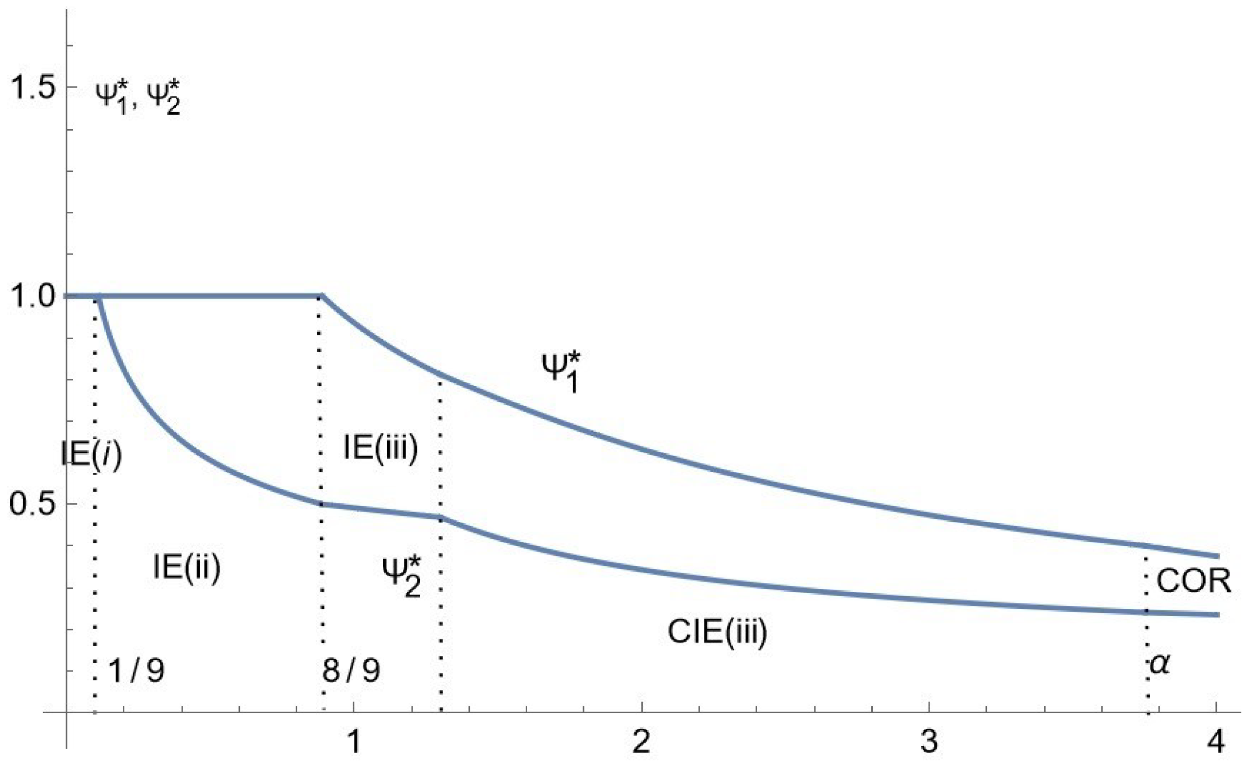
We now deal with four possible cases, depending on whether the constraints are binding or not. One of them turns out to never be possible.
Case (i): Both firms reach all customers.
Both constraints are binding, so that There is a unique solution of Equations (A2)–(A5), which is The condition is necessary and sufficient to ensure that both multipliers are indeed non-negative. Finally, as both , the solution corresponds to a maximum for each firm.
Case (ii): Firm 1 reaches all customers, Firm 2 only a fraction of them.
We must then have and Solving Equations (A2)–(A5), we obtain a unique solution, which is and Notice that is non-negative if , while iff
As both , then the solution corresponds to a maximum for each firm.
Consequently, case (ii) corresponds to an equilibrium if
Case (iii): Both firms reach only a fraction of customers (interior equilibrium).
Here,
Let us first solve for advertising rates as functions of prices. We obtain:
We decompose the reasoning into three steps in order to facilitate the reading.
Step 1: We prove that there is no equilibrium, such that and/or
(a) Consider first
From (
A6), it follows that
Now, from Equations (A4) and (A5),
, so that
Now, from (
A2), for
,
, which implies
and then
(b) Consider then
From (
A2), we obtain
and then
As shown above, however, we cannot have at the equilibrium.
Step 2: A necessary and sufficient condition for the solution.
Substituting the expressions obtained in Equations (A6) and (A7), into Equations (A2) and (A3), and accounting for the fact that
at the equilibrium, one obtains the two equilibrium conditions which the equilibrium prices must satisfy:
and
Subtracting (
A8) from (
A9), one obtains that the following condition must hold at the equilibrium
We can then conclude that the equilibrium prices must satisfy
where
is strictly greater than
and strictly smaller than
14.
Substituting this value for
in (
A9), we obtain that the equilibrium value of
must satisfy:
Let
and
The equilibrium condition (
A11) can be rewritten as:
Step 3: Existence and unity of the solution of Equation (
A12).
Using the above change of variables and
, we can write
Let us then use the equilibrium relationship
to obtain
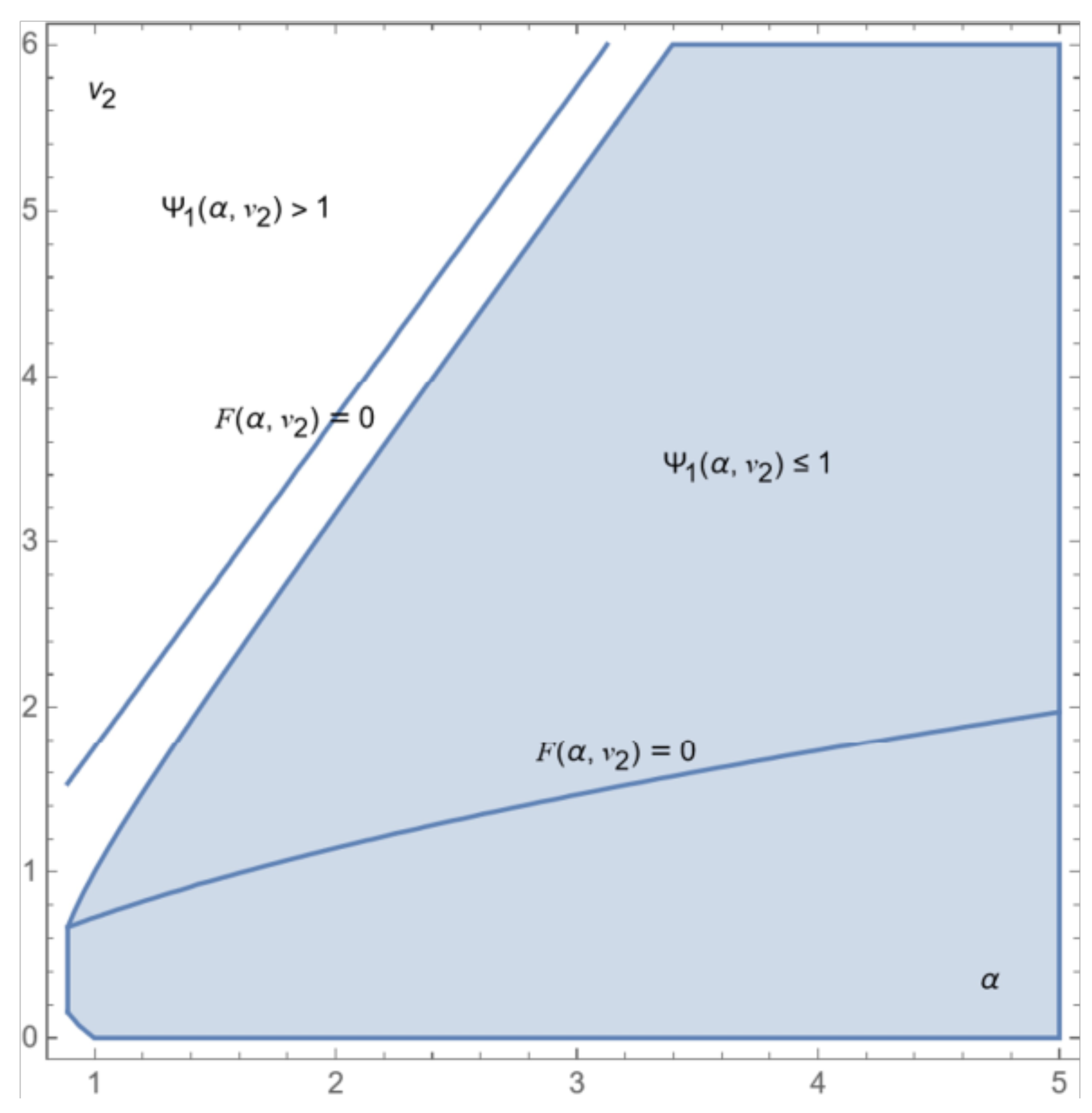
Equation (
A12) has two positive real solutions which are depicted in
Figure A1 in the
-space using the
ContourPlot function of Mathematica. In the same figure, using the
RegionPlot function, we have depicted in blue the area in this space where
It turns out that only the smallest solution of (
A12) (corresponding to the expression of
of case IE (iii) of Proposition 1) is an equilibrium. The greatest one belongs to the white area, where
Figure A1.
Representation in the
-space of Equation (
A12).
Figure A1.
Representation in the
-space of Equation (
A12).
Denoting by
, the equilibrium value from Equation (
A12), we obtain that
= 1 and
for all
We define
similarly to
. We use Equation (A7), giving
as a function of prices, then Equation (
A10) to eliminate
. We use the same change in variables to express
as a function of
and
; finally, we use
, the value of
, satisfying Equation (
A12).
Plotting
and
on the same
Figure A2, for all
, we obtain that (i)
, if and only if
implying that the solution we just described is valid, if and only if,
and (ii)
.
Finally, the obtained are both positive; thus, the obtained solution corresponds to a maximum for each firm.
Case (iv): We prove that there is no equilibrium where Firm 2 reaches all consumers, while Firm 1 reaches only part of them.
Suppose this is the case; we should then have
and
Using the first-order conditions with regards to prices (
A2), we would then obtain:
Substituting for
and
the above values into Equation (A4), we obtain (
):
On the other hand, from Equation (A5), we obtain
From (
A14) one obtains
, where the value of
is the equilibrium candidate value. Substituting this value for
in (
A15), we should have
As pictured in
Figure A3 (representing the expression given in Equation (
A16)), the RHS is always
negative for all values of
Since the multiplier has to be positive, this does not correspond to an equilibrium.
Figure A2.
Representation of the expressions of and as functions of .
Figure A2.
Representation of the expressions of and as functions of .
Figure A3.
Representation of the RHS of Equation (
A16).
Figure A3.
Representation of the RHS of Equation (
A16).
Deviations: We deal with each sub-case of case 1 to prove that no firm admits a profitable deviation.
Case (i): Here, for As long as the price candidates are less than Y, no profitable deviations exist for firms. In fact, each firm’s profit is always null outside of its natural market, as all consumers are informed of the competitor’s product, leaving no room to make a profit on uninformed ones. Hence, for the equilibrium candidate to be an equilibrium, it suffices to have .
Case (ii): Here, there is no possible profitable deviation by Firm 2, since if , for the same reason explained in case (i).
As for Firm 1, as long as , only deviations toward prices may potentially be profitable. But, if , such deviations do not exist at all.
Moreover, we know that
as
. Hence, the interval
has a positive measure and for all
, there is no deviation of Firm 1, showing that a null natural market is possible.
15Case (iii). Here, we have to consider deviations by Firm 1 and Firm 2.
Let us begin with Firm 1. We have to consider deviations in prices , resulting in a null natural market for Firm 1.
We conduct the same reasoning as in case (ii). Noting that , for all , such deviations are not possible.
Let us turn to Firm 2. The prices
, such that Firm 2 has no natural market, satisfy
and provide the firm the profit:
which is maximal at
.
The optimal value in terms of
is equal to
which yields the profit:
It has to be smaller than the candidate equilibrium profit, which can be written as
This is equivalent to
□
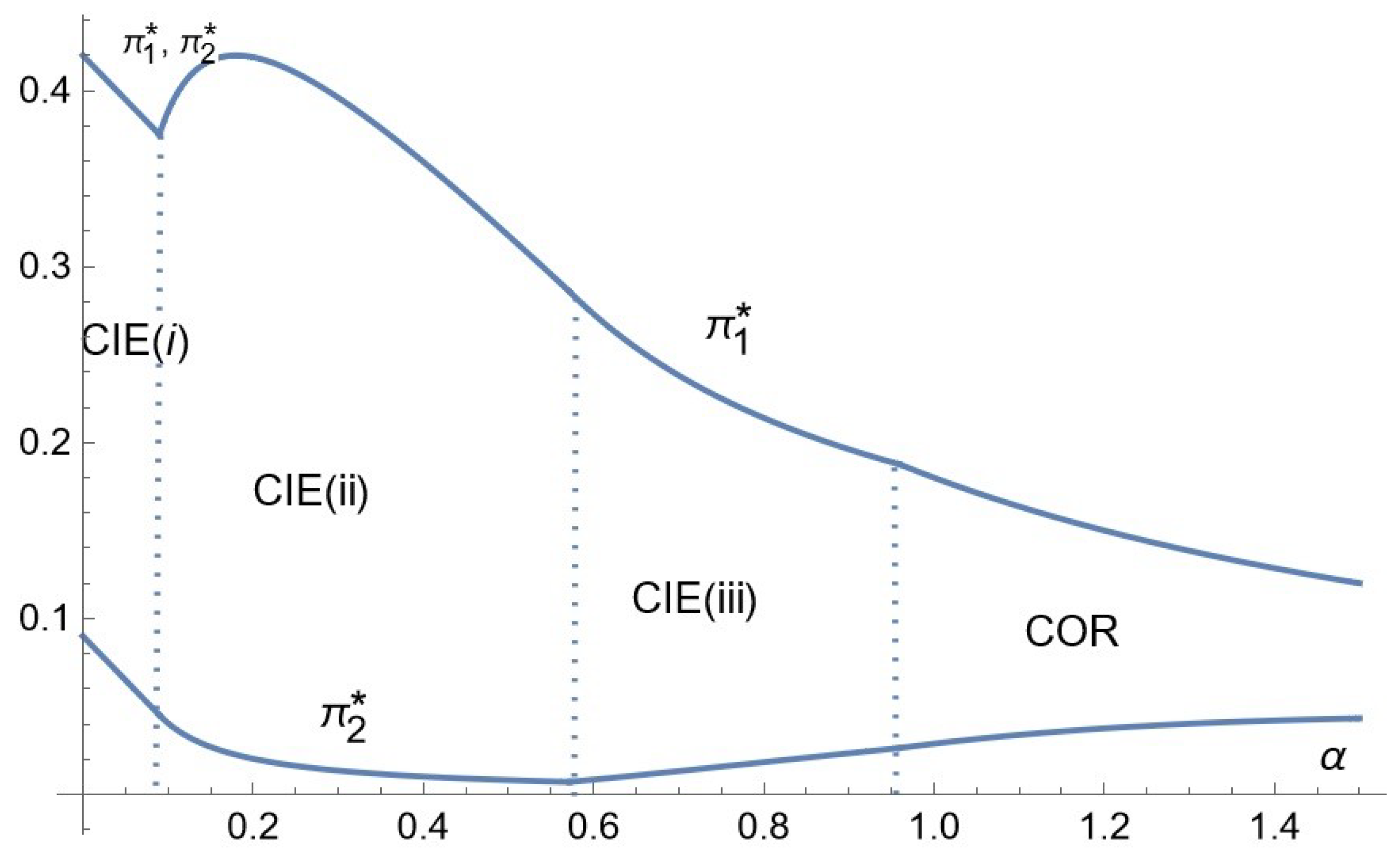
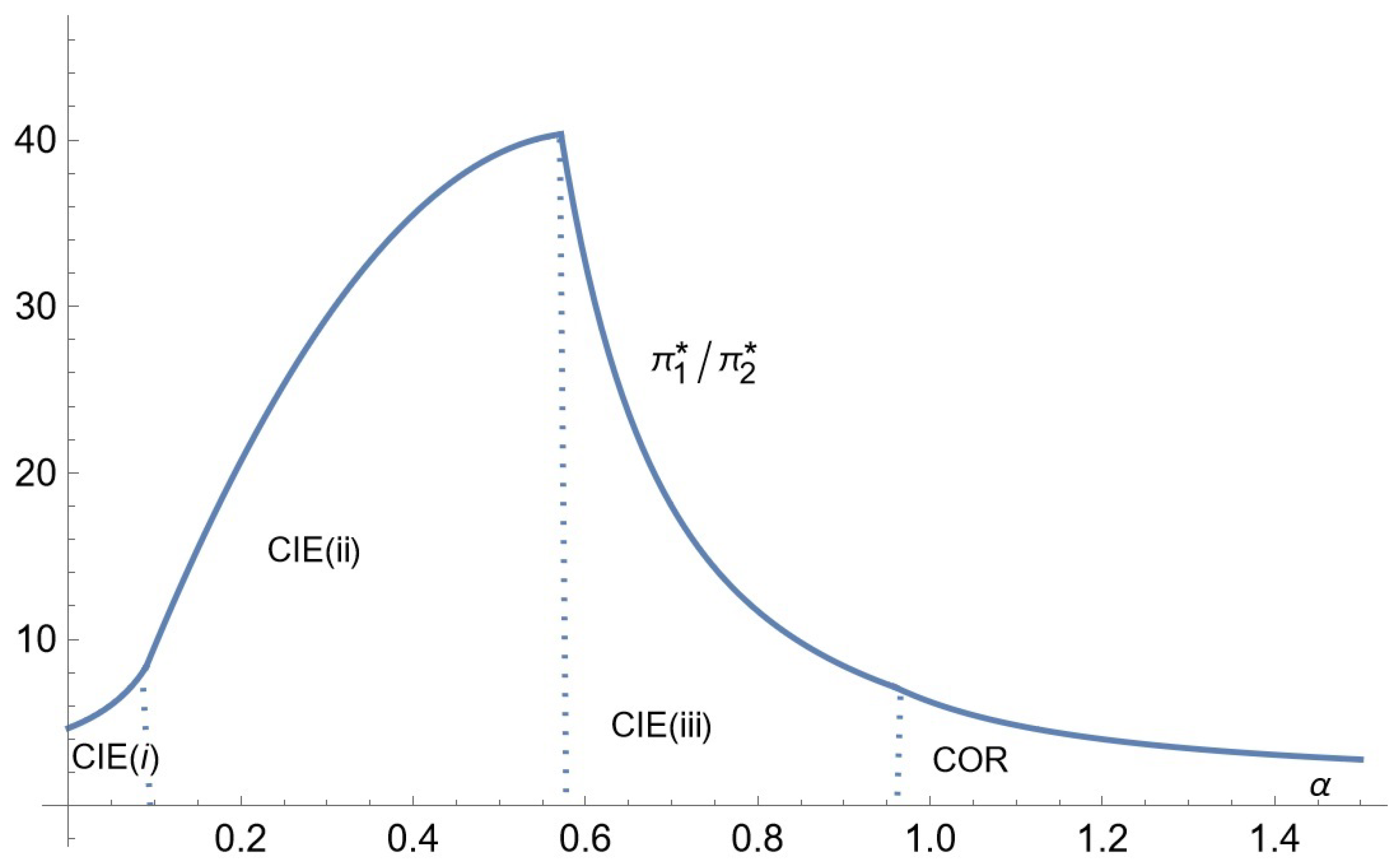
Proof of Proposition 1, Case 2 (CIE). Given the expressions of the profits provided in Equations (3) and (4), the profit maximization by Firms 1 and 2 under the constraints
and
with, respectively, the associated non-negative Lagrangian multipliers
and
, yields the necessary conditions:
We are looking for an equilibrium such that , and each firm has a positive natural market. This necessarily implies , hence .
Now, we consider each possible case, one by one. We first write the first-order conditions allowing us to identify the candidate, then we check the second-order conditions.
(i) For from Equation (A18), one obtains This corresponds to an interior equilibrium only if
The F.O.C. with respect to
(Equation (
A17)), together with the condition
and the expressions of
and
, imply
On the other hand, from condition A19 and the necessary condition , we must have
From condition A20 and the necessary condition , we must have
Notice then that whenever Thus, when , we have .
To sum up, only the conditions are necessary.
The second-order conditions.
For Firm 1, the two constraints are binding, while there are also two variables. Then, we have nothing to check for the second-order conditions.
Firm 2’s bordered Hessian, given that the constraint on
is the only one active, is:
We have to consider the sign of the last principal minor, as there are two variables and one binding constraint. The last principal minor (the third) is equal to , which has the same sign as . Thus, the second-order conditions are satisfied for Firm 2.
(ii) Case and . Conducting the same reasoning as in case (i), we obtain and the necessary condition to have an interior equilibrium.
As , then and Equation (A20) implies which is smaller than 1 iff
Now, from Equation (
A17) and the condition
, we obtain
Using Equation (A19) and the condition , we obtain
Notice, finally, that the latter condition implies
16 .
To sum up, only the conditions and are necessary.
The second-order conditions.
For Firm 1, as in case (i), there is nothing to check, since there are two variables and two binding constraints.
As for Firm 2, given that no constraint is binding, we have to consider the Hessian.
It is obviously a definite negative; thus, the second-order conditions are satisfied as well for Firm 2.
(iii) Case
and
. We have
Using Equations (A19) and (A20) simultaneously, we express
and
, each as a function of the two prices, and thus obtain Equations (
A6) and (A7) again. Then, we substitute these expressions into Equation (A18), which yields Equation (
A9) again, i.e.:
In this equation, substitute
for
,
for
a and
for
, then we obtain condition (
A1).
We are going to show that (1) this equation has one and only one acceptable real positive solution
17 under the conditions indicated in Proposition 1 case CIE (iii); (2) otherwise (when these conditions are not satisfied), either no solution exists or the solution is not acceptable.
The derivative of
with regards to
is given by:
The discriminant of this second-order polynomial is given by , which is of the same sign as . The analysis depends on this sign.
(1) Suppose, first, that , and the discriminant of is always negative; thus, is always decreasing.
The limit of
as
goes to infinity is
. Condition (
A1) has one and only one real non-negative root, if and only if
.
We have
(a) For , simultaneously satisfying and , , the unique real non-negative root of corresponds to an interior equilibrium only if (so that ).
Since is decreasing, in this case, and , then Equation is equivalent to , which writes as , and thus is equivalent to .
In the same way, we use the decrease in , , if and only if , which is equivalent to
We graphically prove that the two conditions and imply the condition
The interior equilibrium identified in case IE (iii) of Proposition 1 corresponds to the solution of the present system that is composed of Equations (
A17)–(A20), with
.
The three Equations (A18)–(A20) are satisfied here in the same way as in case IE (iii). For to correspond to the choice of Firm 1 at the equilibrium, necessarily .
Equation (A18) can we easily be rewritten (replacing
with
y) as
Therefore, is equivalent to .
But, we have supposed
, which implies
for all
. Thus,
. We have
This way, we have shown to be equivalent to
Finally, we consider the value of
, as given by Equation (A7) and substitute
Y for
and
for
We obtain that an inequality
must hold at the equilibrium.
18Graphical analysis
19 shows that
and
g(
hold when
and
Second-order conditions:
Firm 1’s bordered Hessian, given that only the constraint on
is active:
We have to consider the sign of the last principal minor: the determinant of the matrix, which equals , so that the SOC are satisfied for Firm 1.
Firm 2’s Hessian (since no constraint is binding) given by
is a definite negative; thus, the SOC are also satisfied for Firm 2.
(b) For satisfying but , the polynomial is decreasing with , which implies for all . This means that the profit of Firm 2 is decreasing with ; thus, the equilibrium candidate in this case is , , . The inequation is equivalent to . But, implies, on the one hand, , and on the other hand , for which the equilibrium corresponds to case (iii) of the proposition with a positive . Thus, no new case appears with a null price
(2) Suppose now that
,
is a second-degree polynomial that admits two roots:
and
with
.
is positive between the two roots and negative outside, which means that
is decreasing before
, increasing between
and
, and then begins to decrease.
We have that , which is negative when . Polynomial admits potentially three roots, depending on the sign of , and .
When they exist, these roots ( satisfy necessarily , and .
The root , whenever it exists, is never relevant because .
The root
exists, if and only if,
,
. For this root to be acceptable, it must satisfy
, and the multiplier
calculated at
must satisfy
. Recall that
and
The representation of the set of , such that we have, simultaneously , , , and , leads to an empty set.
Finally, regarding , it exists if and only if .
Again, for this root to be acceptable, has to satisfy simultaneously , , and . And, this set is proved, graphically, to be empty.
Deviations. Finally, we have to check that, for each firm, no profitable deviation exists among the prices, such that its natural market is null
20.
For Firm 1, such prices must satisfy , or equivalently . Such prices do not exist as .
As for Firm 2, the prices such that it has no natural market must satisfy , thus , or . But, this price cannot be a profitable deviation for Firm 2 as satisfies the first-order conditions over the segment of prices , and the profit is concave in over this segment; thus, it is decreasing in the neighborhood of y. □
Proof of Proposition 1, Case 3 (corner equilibrium). We deal successively with each possible case: first, when Firm 2 has no natural market, and second, when Firm 1 has no natural market. For each case, we identify the equilibrium candidate, then check whether profitable deviations exist.
(1) If a corner equilibrium exists such that Firm 2 has no natural market, this means that , thus .
We first prove that necessarily
. Indeed, Firm 1’s profit writes:
If ever then, necessarily, , which leads to profit .
Firm 2’s profit writes:
which would be maximal for
. Then, Firm 1 has interest in deviating to a positive price
and a sufficiently small
that ensure a positive
. Thus, necessarily,
.
First, note that necessarily . Indeed, otherwise the best profit in this situation would be , obtained at , whereas Firm 2 may obtain a positive profit if it deviates to a price (which is possible since ) and a sufficiently small .
Hence, is increasing with . Thus, and
Firm 1’s profit
is increasing in
, and then it reaches its maximum at
.
The optimal value of is given by Since , then, necessarily, , or equivalently , which is thus a necessary condition. Hence, we have which implies .
Deviations: For this equilibrium candidate to be an equilibrium, we have to check whether the firms have interest in deviating.
For Firm 1, when
, its profit has only one expression, given by
The best option for Firm 1 in absolute terms is the one provided by the equilibrium candidate. This implies that Firm 1 has no interest in deviating.
As for Firm 2, if
,
If , only the second line of the above profit applies. We have to consider two types of deviations: and , when and only for .
Let us begin with deviations .
The expression of
for
is a continuous and concave function
21 in
, which necessarily reaches its maximum. When an interior solution to the first-order conditions exists, it is the maximum of the function, otherwise the maximum is reached on the borders.
The first-order conditions yield:
For a deviation to a price
to be non-profitable, it is necessary and sufficient that
, which is equivalent to
As
, this implies
. Condition (
A21) is thus more constraining than
, and the couple of conditions reduces to the only condition (
A21).
The proof ends here when .
For
and supposing condition (
A21), we have also to consider deviations to prices
, for which the profit writes:
which increases with
and concave in
. Thus, the best deviation of this nature is
Note that condition (
A21) implies
(or, equivalently,
), so that
The resulting profit is then equal to
which is smaller than the equilibrium candidate profit
, if and only if
But,
, meaning that condition (
A21) implies
This ends the proof for the corner equilibrium, such that Firm 2 has no natural market.
(2) We now deal with possible corner equilibria, such that Firm 1 has no natural market. We first identify the equilibrium candidate; then, we consider deviations. We will prove that the identified equilibrium candidate does not resist to unilateral deviations, thus it is not an equilibrium.
That Firm 1 has no natural market means that , i.e., . This necessarily implies .
Firm 1’s profit is then given by:
Then, necessarily at equilibrium. is then increasing in , thus and
As for Firm 2, with Hence, and , which is necessarily .
At this step, is a necessary condition.
Deviations: Now let us deal with the deviations.
We focus on Firm 2. Firm 2’s profit for all possible prices is given by:
The identified equilibrium candidate corresponds for Firm 2 to the best and for ; thus, there exist no profitable deviations by Firm 2 among these prices.
We now consider the deviations to prices
such that
.
is a concave function in
. The first-order condition with regards to
is independent of
and gives:
For deviations to such prices to be non-profitable, it is necessary and sufficient to have
, which is equivalent to
But, may have two expressions.
When
, then
and Equation (
A22) are equivalent to
or equivalently
.
When
, then
and Equation (
A22) are equivalent to
.
We consider now the deviations of Firm 1. Firm 1’s profit writes:
We consider first the deviations of Firm 1 to prices
, such that
. For such prices,
which is a concave function in
. The first-order condition, with regards to
and independent of
, yields:
For such deviations to be non-profitable, it is necessary and sufficient to have , which is equivalent to .
Considering , the profit is increasing in . When , is increasing for all prices, reaching its maximal value at . Hence, no deviation is profitable for Firm 1. □


