Abstract
Mean-field games (MFGs) are developed to model the decision-making processes of a large number of interacting agents in multi-agent systems. This paper studies mean-field games on graphs (-MFGs). The equilibria of -MFGs, namely, mean-field equilibria (MFE), are challenging to solve for their high-dimensional action space because each agent has to make decisions when they are at junction nodes or on edges. Furthermore, when the initial population state varies on graphs, we have to recompute MFE, which could be computationally challenging and memory-demanding. To improve the scalability and avoid repeatedly solving -MFGs every time their initial state changes, this paper proposes physics-informed graph neural operators (PIGNO). The PIGNO utilizes a graph neural operator to generate population dynamics, given initial population distributions. To better train the neural operator, it leverages physics knowledge to propagate population state transitions on graphs. A learning algorithm is developed, and its performance is evaluated on autonomous driving games on road networks. Our results demonstrate that the PIGNO is scalable and generalizable when tested under unseen initial conditions.
1. Introduction
Multi-agent systems (MAS) are prevalent in engineering and robotics applications. With a large number of interacting agents in the MAS, solving agents’ optimal control could be computationally intractable and not scalable. To solve this challenge, MFGs are [1,2] developed to model strategic interactions among many agents who make dynamically optimal decisions, while a population distribution is propagated to represent the state of interacting agents. Since its inception, MFGs have been widely applied to social networks [3], swarm robotics [4] and intelligent transportation [5,6].
MFGs are micro-macro games that bridge agent dynamics and population behaviors with two coupled processes: individuals’ dynamics solved by optimal control (i.e., agent dynamic) and system evolution arising from individual choices (i.e., population behaviors).
In this work, we focus on a class of MFGs [7], namely, mean-field games on graphs (-MFG), where the state space of the agent population is a graph and agents select a sequence of nodal and edge transitions with a minimum individual cost. Solving these -MFGs, however, poses the following challenges: (1) With a graph-based state space, the action space expands significantly, encompassing both nodes and edges, resulting in a high-dimensional search space. More specifically, the decision-making of a representative agent in -MFG consists of not only en-route choices at nodes but also continuous velocity control on edges subject to congestion effects. (2) Existing work mainly assumes that the initial population distribution is fixed. The change in initial population states leads to the re-computation of mean-field equilibria (MFE), a task that requires computational and memory resources and hinders the practicality of deploying MFG solutions.
To address these challenges, this paper proposes a new learning tool for -MFGs, namely, a physics-informed graph neural operator (PIGNO). The key element is a graph neural operator (GNO), which can generate population dynamics given the initial population distribution. To enhance the training process, the GNO incorporates physics knowledge regarding how agent and population dynamics propagate over the spatiotemporal domain.
Related Work
Researchers have explored various machine learning methods, such as reinforcement learning (RL) [8,9,10,11], and physics-informed neural networks (PINN) [12,13,14]. However, it can be time-consuming and memory-demanding for these learning tools to adapt to changes in initial population density. Specifically, each unique initial condition may require the assignment and retraining of a dedicated neural network to obtain the corresponding MFE. To enhance the scalability of the learning framework for MFGs, Chen et al. [15] introduced a physics-informed neural operator (PINO) framework. This framework utilizes a Fourier neural operator (FNO) to establish a functional mapping between mean-field equilibrium and boundary conditions. However, the FNO fails to solve -MFGs because it cannot directly project information over a graph into a high-dimensional space and generate population dynamics in the graph state space. Therefore, in this paper, we propose a graph neural operator (GNO) that learns mappings between graph-based function spaces to solve -MFGs. The GNO leverages message-passing neural networks (MPNNs) to handle state space and propagate state information efficiently by aggregating the neighborhood messages.
Our contributions include: (1) We propose a scalable learning framework leveraging PIGNO to solve -MFGs with various initial population states; (2) We develop a learning algorithm and apply it to autonomous driving games on road networks to evaluate the algorithm performance.
2. Background
2.1. Mean-Field Games on Graphs (-MFG)
Mean-field games on graphs (-MFG) model population dynamics and a generic agent’s optimal control on both nodes and edges. A -MFG consists of a forward FPK and multiple backward HJB equations, which are defined on a graph as follows:
Definition 1.
A -MFG with discrete time graph states [16] is:
is the population density on each edge at time step . denotes the initial population density over the graph. The Fokker–Planck (FPK) equation captures the evolution of the population state on the graph. The Hamilton–Jacobi–Bellman (HJB) equation captures the optimal control of a generic agent, including the velocity control on edges and route choice on nodes. is the value function at each edge. denotes the terminal cost. denotes the exit rate at each edge, which represents the agent’s velocity control. is the probability of choosing node j as the next-go-to node at node i, i.e., route choice. is the cost incurred by the agent at time step . The transition matrix is determined by and . The MFE is denoted by , satisfying Equation (1). The mathematical details of -MFG can be found in Appendix A.1. We provide a toy example in Appendix A.2 to help readers better understand it.
2.2. Graph Neural Operator (GNO)
Graph neural operators (GNOs) are generalized neural networks that can learn functional mappings between high-dimensional spaces [17]. GNO utilizes an MPNN to update space representation according to messages from the neighborhood. In this paper, we adopt a GNO to establish mappings between initial population state and population at MFE. We leverage the physics knowledge (i.e., FPK and HJB equations) to train the GNO for solving MFE with various initial population densities, eliminating the need to recompute MFE.
3. Scalable Learning Framework
In this section, we propose a physics-informed graph neural operator (PIGNO) to learn -MFGs. Figure 1 illustrates the workflow of two couple modules: FPK for population behaviors and HJB for agent dynamics. The FPK and the HJB modules internally depend on each other. In the FPK module, we estimate population density over the graph and update the GNO using a residual defined by the physical rule that captures population dynamics triggered by the transition matrix defined in the FPK equation. In the HJB module, the transition matrix is obtained given the population density . We adopt another GNO to solve the HJB equation since the dynamics of the agents and the cost functions are known in the MFG system. We now delve into the details of the proposed PIGNO.
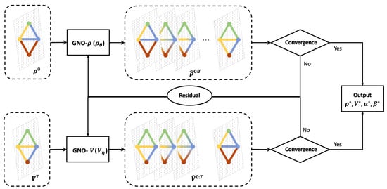
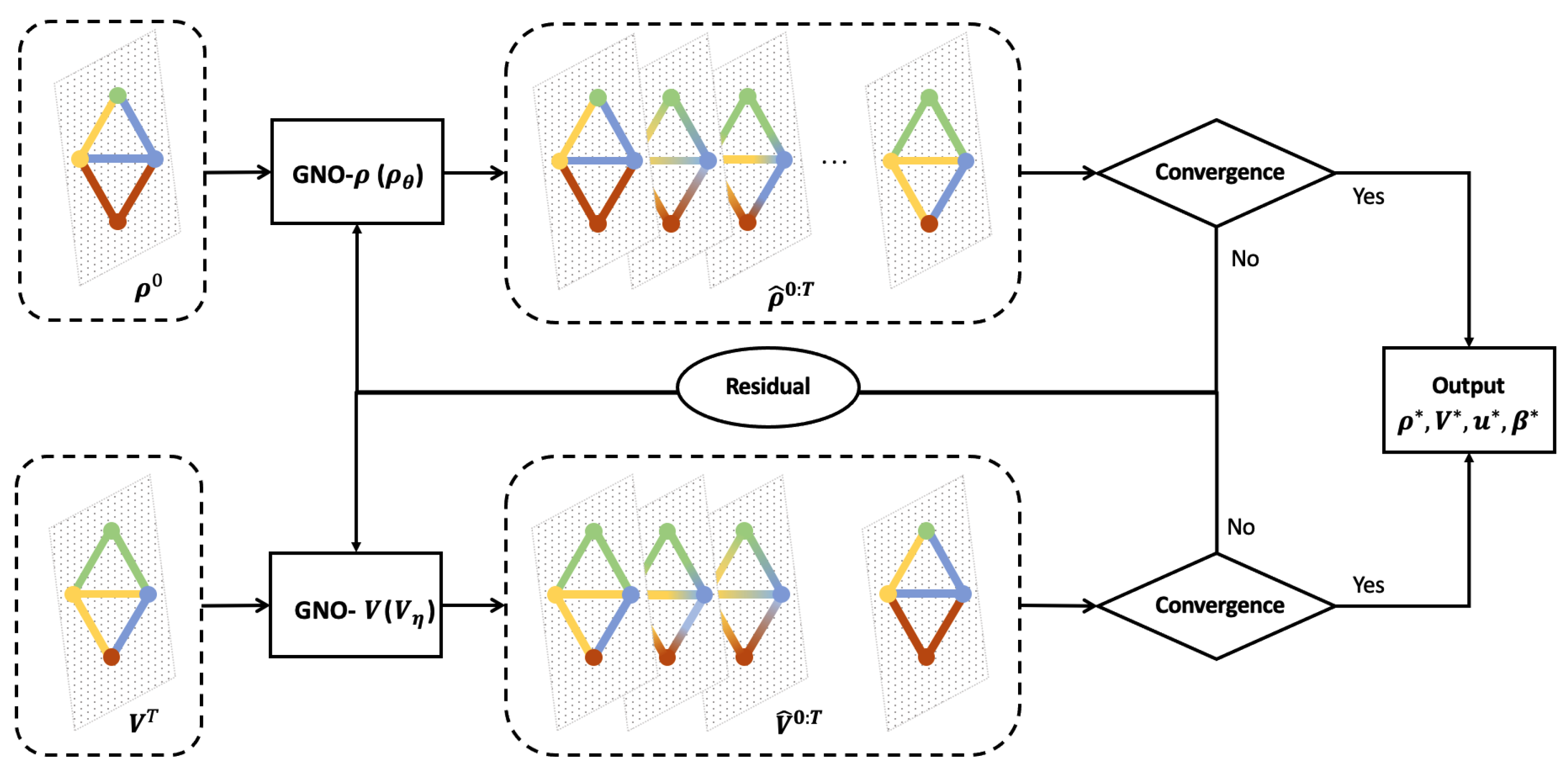
Figure 1.
PIGNO for -MFGs: We leverage graph neural networks to establish a functional mapping between the initial population density along with terminal cost and mean field equilibrium over the entire spatial temporal domain. The population density and terminal cost over the space domain at each time step is denoted by color bars over the graph. The PIGNO allows us to obtain MFEs corresponding to each initial population distribution and terminal cost without recomputing them.
3.1. PIGNO for Population Behaviors
The GNO- maps the initial population distribution and the population distribution from time 0 to T. The input of GNO- is the initial population density along with the transition information to propagate population dynamics. The output of GNO- is the population dynamics over the spatiotemporal domain, denoted by . The PIGNO is instantiated as the following MPNN:
where, is the population density of edge at time , is the set of neighborhood edges of edge at time , is the graph kernel function for , and denotes the cumulative message used to propagate population dynamics from time 0 to time . indicates the ratio of the population entering from edge to edge till time , which is determined by the ratio of population exiting the edge (i.e., the velocity control u) and the ratio of the population choosing the edge as the next-go-to edge (i.e., the route choice ). The MPNN utilizes the initial population distribution and the message to propagate the population dynamics in the -MFG system. The neighborhood message is transformed by a kernel function and aggregated as an additional feature to estimate population density.
The GNO- adopts a physics-informed training scheme, which combines both model-driven and data-driven methods. The training of GNO- is guided by the residual determined by physical rules of population dynamics. Mathematically, the residual is:
where, the set contains various initial densities over the graph. is calculated as:
where, the first term in evaluates the physical discrepancy based on Equation (1a). It integrates the residual of the FPK equation, ensuring that the model adheres to established laws of motion. When predicted becomes closer to satisfying the FPK equation, the residual gets closer to 0. The second term quantifies the discrepancy between the estimations and the ground truth of the initial density. The observed data comes from the initial distribution of population . The training of based on observed data follows the traditional supervised learning scheme. and are the weight coefficients.
3.2. PIGNO for Optimal Control
Similar to GNO-, GNO-V learns a reverse mapping from the terminal costs to the value functions over the graph from time T to 0. The input of GNO-V is the terminal costs and the transition information. The output of GNO-V is the value function over the spatiotemporal domain, denoted by . The GNO-V also follows the MPNN formulation:
where is the value function of edge at time , is the set of neighborhood edges of edge at time , is the graph kernel function for , and denotes the cumulative message used to propagate population dynamics from time 0 to time , which comes from the transpose of the cumulative transition matrix in GNO-. The MPNN utilizes the terminal costs and the message to propagate system value functions. The neighborhood message is transformed by a kernel function and aggregated as an additional feature to estimate value functions.
The training of GNO-V takes the HJB residual into consideration, which is
where, the set contains various terminal costs over the graph. is calculated as:
where, the first term in evaluates the physical discrepancy based on Equation (1b). When predicted becomes closer to the optimal , the residual gets closer to 0. The second term calibrates the predictions to the ground truth of the terminal costs by supervised learning. Similarly, and are the weight coefficients.
Note that a meta assumption of this model is discrete time. There are significant limitations of adopting a continuous-time model: (1) A continuum formulation of forward process over a graph space cannot be easily captured by several coupled partial differential equation systems. One way is to simplify the decision making over the graph as discretized route choice at each node, rendering the game as a continuous time markov decision process, which fails to capture the real-time velocity control on each edge. The other way is to formulate the dynamic process as a graph ODE, which requires further investigation on scalability. (2) A continuum formulation of backward process can be solved by continuous-time reinforcement learning. We leave the scalability of this continuous time reinforcement learning scheme to future work.
4. Solution Approach
In this section, we present our learning algorithm (Algorithm 1). We first initialize the GNO- parameterized by and GNO-V parameterized by . During the ith iteration of the training process, we first sample a batch of initial population densities and terminal costs . The terminal cost denotes the delay for agents who haven’t arrived at their destinations at the terminal time step. In this work, we assume the time delay at the terminal step is proportional to the travel distance between the agent’s location and her destination. represents the set of initial population density. In this work, we interpret initial population density as the travel demands (i.e., the number of agents entering a graph at time 0). Agents can enter the graph from each node. We assume at time 0, the number of agents at each node (i.e., travel demand) follow a uniform distribution. We use each pair of and to generate the population density and over the entire domain. Given and , we obtain the spatiotemporal transition P for all nodes. We then update the parameter of the neural operator according to the residual. At the end of each iteration, we check the convergence according to:
| Algorithm 1 PIGNO-MFG |
|
5. Numerical Experiments
In this section, we employ our algorithm to facilitate autonomous driving navigation in traffic networks. As illustrated in Figure 2, a substantial number of autonomous vehicles (AVs) move to destination node 4, with the objective of minimizing total costs subject to the congestion effect. We use a representative agent as an example to elaborate on the speed control and density dynamics of the population in this scenario. At node 1, the representative agent first selects edge . The agent then drives along edge and selects continuous-time-space driving velocities on the edge. The agent selects her next-to-go edge at node 2, following this pattern until she reaches her destination at node 4. These choices regarding her route and speed will actively influence the evolution of population density across the network. The mathematical formulation of this autonomous driving game can be found in [16].
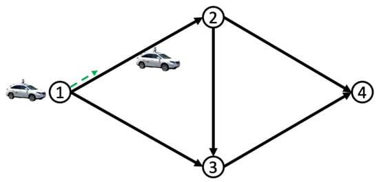
Figure 2.
Autonomous driving game on the road network.
We construct the initial population state over the network as follows: We assume that at time 0, the traffic network is empty. Vehicles enter the road network at origin nodes and move toward the destination 4. Travel demands at each origin satisfy . Therefore, each initial population distribution over the network consists of travel demands at origins (i.e., ), which are sampled from three independent uniform distributions.
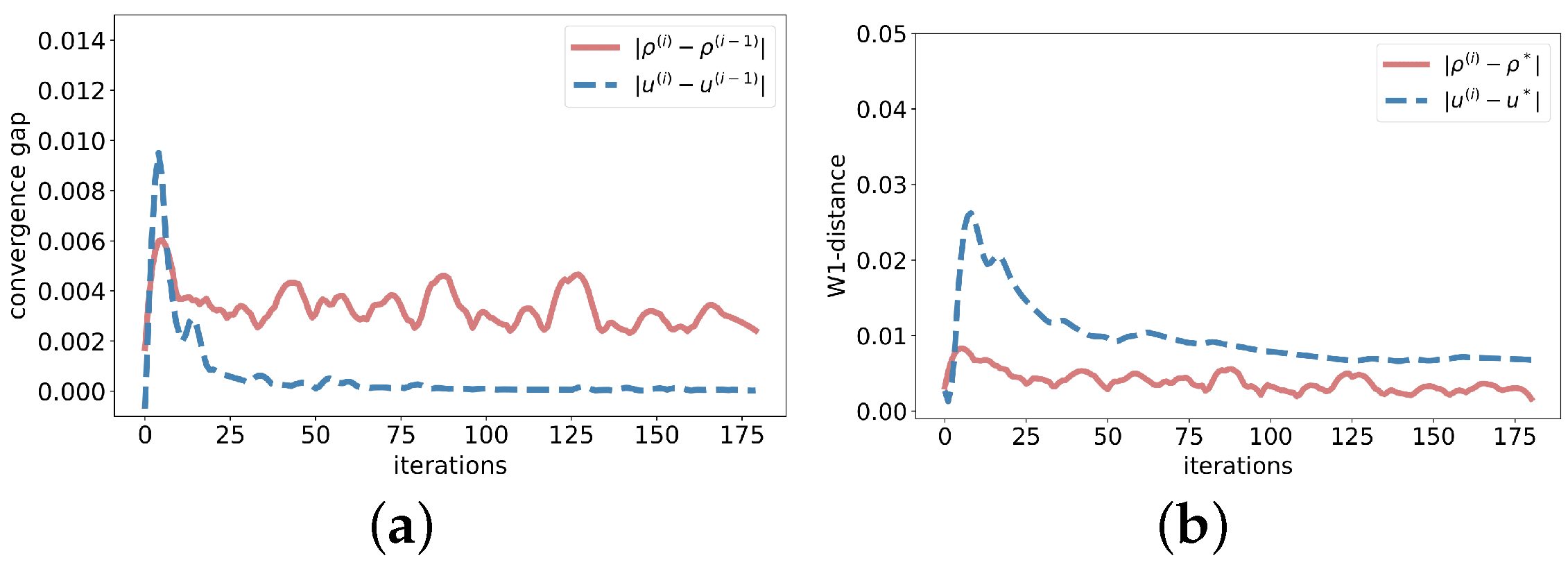
Figure 3 demonstrates the convergence performance of the algorithm in solving -MFG. The x-axis represents the iteration index during training, the y-axis displays the convergence gap, and the 1-Wasserstein distance measures the closeness between our results and the MFE obtained by numerical methods [16]. The results demonstrate that our algorithm can converge stably after 50 iterations.
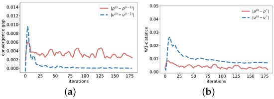
Figure 3.
Algorithm performance (a) Convergence gap (b) W1-distance.
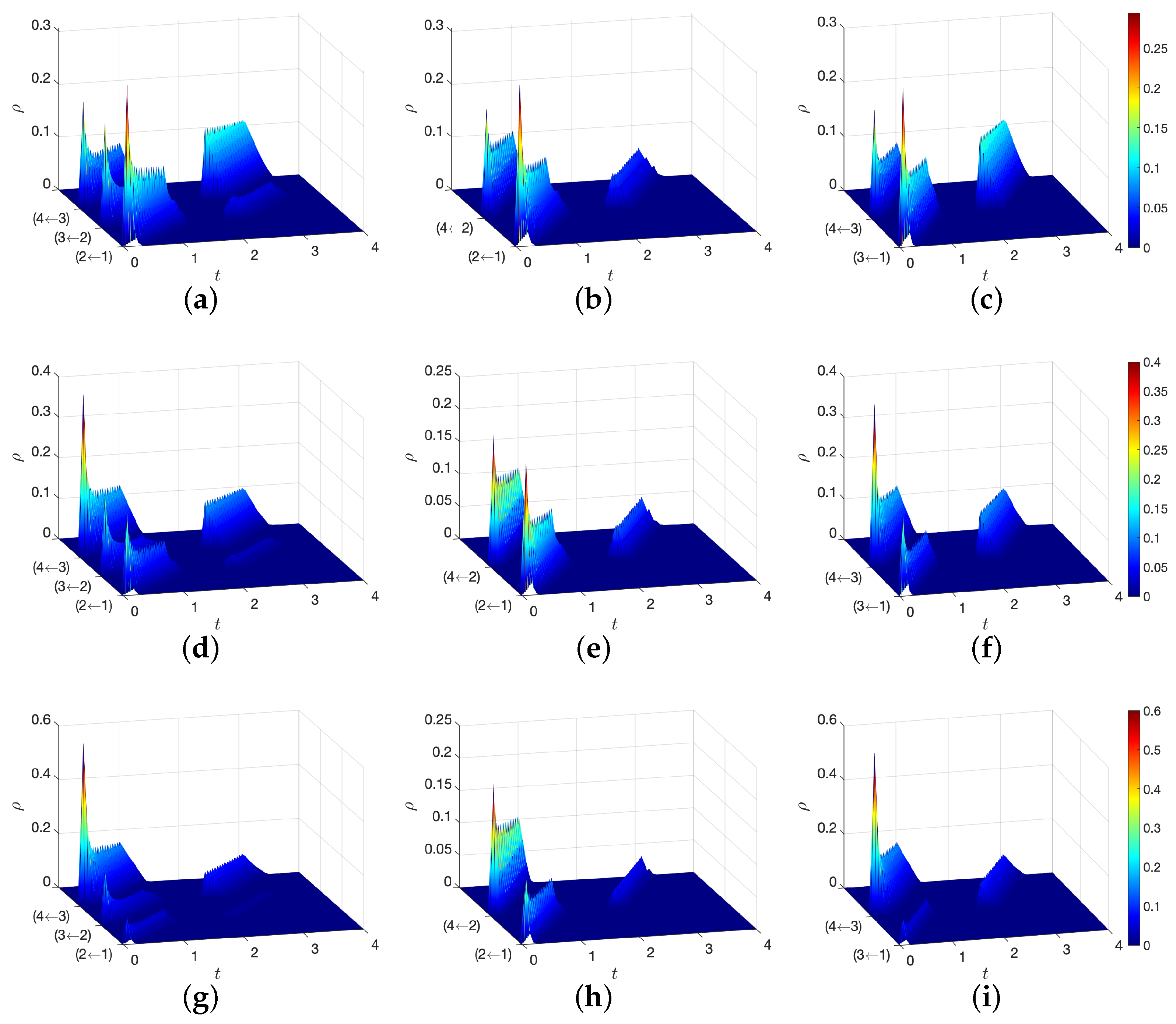
Figure 4 demonstrates the population density solved by our proposed method along three paths on the road network, i.e., , , and . The x-axis is the spatial position on the path, and the y-axis represents the time. The z-axis represents the population density . The running cost functional form follows a non-separable cost structure with a crossing term of the agent action and the population density. We visualize the population density in -MFG with three initial population states, which are constructed by travel demands : (See Figure 4a–c), (See Figure 4d–f) and (See Figure 4g–i). The plots show the population density evolution along each path on the graph. At the node, the density flow can be split when making route choice. For example, at node 2, vehicles can choose node 3 or 4 as their next node. It means the vehicle flow on the edge (1,2) is split into flows on edges (2,3) and (2,4).
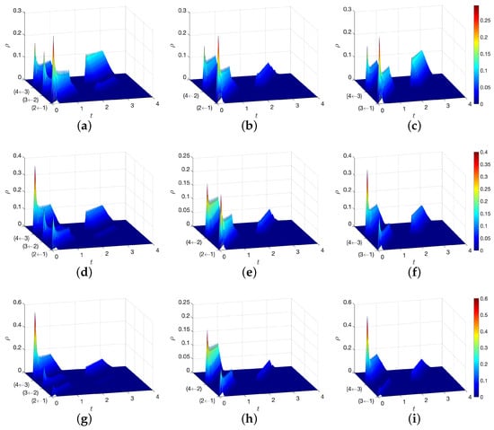
Figure 4.
Population density along each path on the road network with various travel demands . (a) (b) , demand: (c) (d) (e) , demand: (f) (g) (h) , demand: (i) .
6. Conclusions
In this paper, we propose a scalable learning framework, -MFGs. Existing numerical methods have to recompute MFE when the initial population density changes. To avoid recomputing MFE inefficiently, this work proposes a learning method, which utilizes graph neural networks to establish a functional mapping between the initial population density and MFE over the entire spatial temporal domain. This learning framework allows us to obtain MFEs corresponding to each initial population distribution without recomputing them. We demonstrate the efficiency of this method in autonomous driving games. Our contribution lies in the scalability of PIGNO to handle various initial population densities without recomputing MFEs. Our framework offers a memory- and data-efficient approach for solving -MFGs.
Author Contributions
Conceptualization, X.C.; methodology, S.L. and X.C.; validation, S.L. and X.C.; writing—original draft preparation, S.L. and X.C.; writing—review and editing, X.C. and X.D.; visualization, S.L.; supervision, X.D.; project administration, X.D.; funding acquisition, X.D.; S.L. and X.C. have the equal contribution to this paper. All authors have read and agreed to the published version of the manuscript.
Funding
This work is partially supported by the National Science Foundation CAREER under award number CMMI-1943998.
Data Availability Statement
No new data were created or analyzed in this study. Data sharing is not applicable to this article.
Conflicts of Interest
The authors declare no conflict of interest. All authors have approved the manuscript and agree with its submission to the journal “Games”.
Appendix A
Appendix A.1. Mean Field Games on Graph
Optimal control of a representative agent: On a graph , a generic agent moves from her initial position to a destination, aiming to solve optimal control to minimize its cost connecting its origin to the destination. Assume there is a single destination for all the agents. One with multiple destinations forms a multi-population MFG and will be left for future research. The agent’s state at time t can be specified by two scenarios, either in the interior of an edge or at a node. In the interior of edge : is the agent’s position on edge l at time t where and is the length of edge l. is the velocity of the agent at position x at time t when navigating edge l. Note that -MFG is non-stationary, thus, the optimal velocity evolves as time progresses. is the congestion cost arising from the agent population on edge l, which is increasingly monotone in indicating the congestion effect. is the minimum cost of the representative agent starting from position x at time t. is modeled by a HJB equation: ,
where, are partial derivatives of with respect to , respectively. represent the edges going into node i. is the minimum travel cost of agents staring from node i (i.e., the end of edge l) at time t, which is also the boundary condition of Equation (A1). At node : represents the probability of choosing the next-go-to edge where represent the edges coming out of node i. We have . can be interpreted as the proportion of agents selecting edge l (or turning ratio) at node i at time t. determines the boundary condition of population evolution on edges, which will be defined in Equation (A7). is the minimum traverse cost starting from node i at time t. satisfies
where, is the minimum cost entering edge l (i.e., ) at time t. is the terminal cost at destination s.
We now show Equations (A1) and (A2) can be reformulated into Equation (1b) in a discrete-time setting. We first discretize the spatiotemporal domain. On a spatiotemporal mesh grid, denote as the spatial and temporal mesh sizes, respectively. Denote as the discretized representation of . To construct from , we first discretize edges on a graph. Each edge is divided into a sequence of adjacent edge cells, denoted as , where is the number of adjacent edge cells. The node set is created by augmenting with auxiliary nodes that separate newly split edge cells. In summary, a spatially discretized directed graph is a collection of edge cells and augmented nodes linked by directed arrows. It preserves the topology of the original graph but with more edges and nodes. We discretize the time interval into , where represents the discretized time instant. The relation between the spatial and temporal resolutions needs to fulfill the Courant–Friedrichs–Lewy (CFL) condition to ensure numerical stability: , where is the maximum velocity. We first reformulate Equation (A1) on spatiotemporal grids where as follows
On the graph , . We have where is the successor edge cell of in the interior of an edge. Therefore,
where, .
Edge cell are the last cell on an edge and j is the end node of the edge. It means j is also the start node of the next-go-to edge. We have . Accordingly,
We then look into Equation (A2). We denote and we assume that agents entering node i and making route choice at time will exist the node at time . We then have . Therefore,
We substitute in Equation (A3) with V according to Equation (A4) and obtain Equation (1b). We have .
where, is a successor edge cell of . Below we show that is a transition matrix. For diagonal elements of , , we have
For off-diagonal elements,
The sum of elements in each row is:
Therefore, is a transition matrix satisfying: (1) each element is between 0 and 1, and (2) the sum of elements in each row equals 1.
Population dynamics: When all agents follow the optimal control, the population density distribution on edge l, denoted as , evolves over the graph. It is solved by a deterministic (or first-order) FPK, given the velocity control of agents:
where are partial derivatives of with respect to , respectively. Since agents may not appear or disappear randomly, there is no stochasticity in this equation. is the initial population density. At the starting node of edge l or the starting position on edge l, agents move to the next-go-to edge based on their route choice. Therefore, the boundary condition is:
where, and is the influx entering edge l at time t. For a source node where new agents appear, this node can be treated as a dummy edge where agents exit this edge at a speed of to enter a downstream edge. In the above boundary condition, there is no need to distinguish between an intermediate and a source node explicitly without loss of generality.
Appendix A.2. Toy Example
To further demonstrate the linkage of these MFGs on graphs, below we present a toy network (Figure A1) and show how each model is formulated on this network.
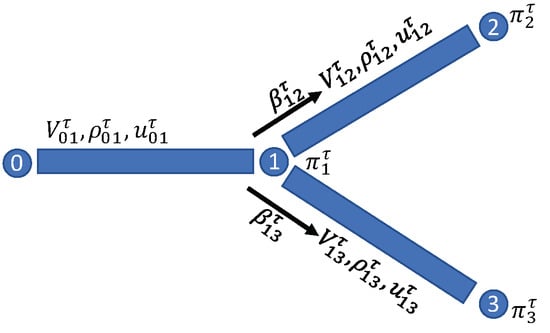
Figure A1.
Toy example.
Figure A1.
Toy example.
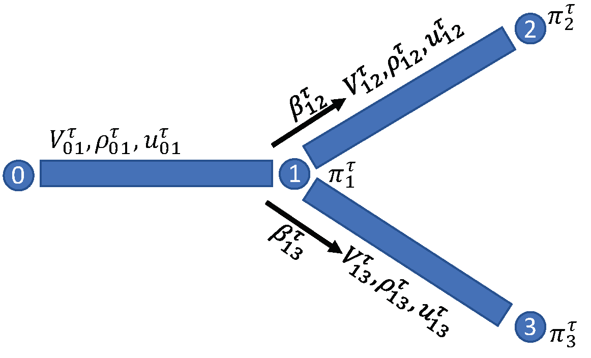
The -dMFG on the toy network is first presented. We assume and . We have
We have
References
- Lasry, J.M.; Lions, P.L. Mean field games. Jpn. J. Math. 2007, 2, 229–260. [Google Scholar] [CrossRef]
- Huang, M.; Malhamé, R.P.; Caines, P.E. Large population stochastic dynamic games: Closed-loop McKean-Vlasov systems and the Nash certainty equivalence principle. Commun. Inf. Syst. 2006, 6, 221–252. [Google Scholar]
- Yang, J.; Ye, X.; Trivedi, R.; Xu, H.; Zha, H. Deep Mean Field Games for Learning Optimal Behavior Policy of Large Populations. In Proceedings of the International Conference on Learning Representations, Vancouver, BC, Canada, 30 April–3 May 2018. [Google Scholar]
- Elamvazhuthi, K.; Berman, S. Mean-field models in swarm robotics: A survey. Bioinspir. Biomim. 2019, 15, 015001. [Google Scholar] [CrossRef] [PubMed]
- Calderone, D.; Sastry, S.S. Markov Decision Process Routing Games. In Proceedings of the 8th International Conference on Cyber-Physical Systems, ICCPS ’17, Pittsburgh, PA, USA, 18–20 April 2017; Association for Computing Machinery: New York, NY, USA, 2017. [Google Scholar]
- Cabannes, T.; Laurière, M.; Perolat, J.; Marinier, R.; Girgin, S.; Perrin, S.; Pietquin, O.; Bayen, A.M.; Goubault, E.; Elie, R. Solving N-Player Dynamic Routing Games with Congestion: A Mean-Field Approach. In Proceedings of the 21st International Conference on Autonomous Agents and Multiagent Systems, AAMAS ’22, Auckland, New Zealand, 9–13 May 2022. [Google Scholar]
- Guéant, O. Existence and uniqueness result for mean field games with congestion effect on graphs. Appl. Math. Optim. 2015, 72, 291–303. [Google Scholar] [CrossRef]
- Guo, X.; Hu, A.; Xu, R.; Zhang, J. Learning Mean-Field Games. In Advances in Neural Information Processing Systems (NeurIPS 2019); Curran Associates, Inc.: New York, NY, USA, 2019. [Google Scholar]
- Subramanian, J.; Mahajan, A. Reinforcement Learning in Stationary Mean-Field Games. In Proceedings of the 18th International Conference on Autonomous Agents and MultiAgent Systems, AAMAS ’19, Montreal, QC, Canada, 13–17 May 2019; pp. 251–259. [Google Scholar]
- Perrin, S.; Laurière, M.; Pérolat, J.; Élie, R.; Geist, M.; Pietquin, O. Generalization in Mean Field Games by Learning Master Policies. Proc. Aaai Conf. Artif. Intell. 2022, 36, 9413–9421. [Google Scholar] [CrossRef]
- Lauriere, M.; Perrin, S.; Girgin, S.; Muller, P.; Jain, A.; Cabannes, T.; Piliouras, G.; Perolat, J.; Elie, R.; Pietquin, O.; et al. Scalable Deep Reinforcement Learning Algorithms for Mean Field Games. In Proceedings of the 39th International Conference on Machine Learning, PMLR, Baltimore, MD, USA, 17–23 July 2022; Volume 162, pp. 12078–12095. [Google Scholar]
- Ruthotto, L.; Osher, S.J.; Li, W.; Nurbekyan, L.; Fung, S.W. A machine learning framework for solving high-dimensional mean field game and mean field control problems. Proc. Natl. Acad. Sci. USA 2020, 117, 9183–9193. [Google Scholar] [CrossRef] [PubMed]
- Carmona, R.; Laurière, M. Convergence Analysis of Machine Learning Algorithms for the Numerical Solution of Mean Field Control and Games I: The Ergodic Case. SIAM J. Numer. Anal. 2021, 59, 1455–1485. [Google Scholar] [CrossRef]
- Germain, M.; Mikael, J.; Warin, X. Numerical resolution of McKean-Vlasov FBSDEs using neural networks. Methodol. Comput. Appl. Probab. 2022, 24, 2557–2586. [Google Scholar] [CrossRef]
- Chen, X.; Fu, Y.; Liu, S.; Di, X. Physics-Informed Neural Operator for Coupled Forward-Backward Partial Differential Equations. In Proceedings of the 1st Workshop on the Synergy of Scientific and Machine Learning Modeling@ICML2023, Honolulu, HI, USA, 28 July 2023. [Google Scholar]
- Chen, X.; Liu, S.; Di, X. Learning Dual Mean Field Games on Graphs. In Proceedings of the 26th European Conference on Artificial Intelligence, ECAI ’23, Kraków, Poland, 30 September–5 October 2023. [Google Scholar]
- Li, Z.; Kovachki, N.; Azizzadenesheli, K.; Liu, B.; Bhattacharya, K.; Stuart, A.; Anandkumar, A. Multipole Graph Neural Operator for Parametric Partial Differential Equations. In Proceedings of the 34th International Conference on Neural Information Processing Systems, Online, 6–12 December 2020; Curran Associates, Inc.: New York, NY, USA, 2020. NIPS’20. [Google Scholar]

Disclaimer/Publisher’s Note: The statements, opinions and data contained in all publications are solely those of the individual author(s) and contributor(s) and not of MDPI and/or the editor(s). MDPI and/or the editor(s) disclaim responsibility for any injury to people or property resulting from any ideas, methods, instructions or products referred to in the content. |
© 2024 by the authors. Licensee MDPI, Basel, Switzerland. This article is an open access article distributed under the terms and conditions of the Creative Commons Attribution (CC BY) license (https://creativecommons.org/licenses/by/4.0/).